Abstract
Quantification of vegetation biophysical variables such as leaf area index (LAI), fractional vegetation cover (fCover), and biomass are among the key factors across hydrological, agricultural, and irrigation management studies. The present study proposes a kernel-based machine learning algorithm capable of performing adaptive and nonlinear data fitting so as to generate a suitable, accurate, and robust algorithm for spatio-temporal estimation of the three mentioned variables using Sentinel-2 images. To this aim, Gaussian process regression (GPR)–particle swarm optimization (PSO), GPR–genetic algorithm (GA), GPR–tabu search (TS), and GPR–simulated annealing (SA) hyperparameter-optimized algorithms were developed and compared against kernel-based machine learning regression algorithms and artificial neural network (ANN) and random forest (RF) algorithms. The accuracy of the proposed algorithms was assessed using digital hemispherical photography (DHP) data and destructive measurements performed during the growing season of silage maize in agricultural fields of Ghale-Nou, southern Tehran, Iran, in the summer of 2019. The results on biophysical variables against validation data showed that the developed GPR-PSO algorithm outperformed other algorithms under study in terms of robustness and accuracy (0.917, 0.931, 0.882 using R2 and 0.627, 0.078, and 1.99 using RMSE in LAI, fCover, and biomass of Sentinel-2 20 m, respectively). GPR-PSO also possesses the unique ability to generate pixel-based uncertainty maps (confidence level) for prediction purposes (i.e., estimated uncertainty level <0.7 in LAI, fCover, and biomass, for 96%, 98%, and 71% of the total study area, respectively). Altogether, GPR-PSO appears to be the most suitable option for mapping biophysical variables at the local scale using Sentinel-2 images.
1. Introduction
An essential step in monitoring cropland properties, modeling crop growth, and forecasting yield, optimizing crop production [1], and improving crop field management [2] during the growing season involves the space-based estimation of key canopy biophysical variables such as leaf area index (LAI), fractional vegetation cover (fCover), and biomass [3].
LAI and fCover characterize the vegetation cover structure [4] and energy absorption capacity of the canopy, and so are indispensable in most global climate models, as well as studies on hydrology, ecology, and agro–ecosystems [5]. These variables also play crucial roles in the estimation of aboveground biomass and vegetative evapotranspiration [6].
Traditionally, the estimation of these variables was conducted via in situ destructive methods, which of course are very time-consuming and costly. However, recent algorithms based on remote sensing data are employed for retrieving biophysical variables [7]. Optical remote sensing has proved its potential for quantitative and continuous spatio-temporal retrieval of key canopy characteristics [8]. Following the launch of the super-spectral Copernicus Sentinel-2 (S2) missions, unprecedented data streams for land monitoring [9] also became readily available, ensuring the development of spatio-temporal quantitative retrieval techniques deemed necessary among remote sensing communities [10,11,12].
Yet, widely accepted empirical methods remain prone to unstable performance in different case studies, and are limited to 2–5 bands, making it unclear whether the best band combinations are being employed; in addition, vegetation indices (VIs) are considerably affected by additional confounding factors such as vegetation structure and background at canopy level [13,14,15]. Conversely, physically based methods such as inverting a radiative transfer model (RTM) are computationally demanding and require further site-specific information simultaneously for proper model parameterization, which is not always instantly available, accurate, or up-to-date. The quality of such methods relies upon prior knowledge and regularization [3]. However, machine learning regression algorithms (MLRAs) can generate adaptive and robust relationships in a given study area and are easily applicable with less site-specific information [16]. MLRAs can typically cope with strong nonlinearity arising out of the functional dependence between biophysical variables and the observed reflected radiance [15,17], as nonlinear relationships are often the case in multi- or hyperspectral imagery [3]. Kernel-based MLRAs involve few and intuitive hyperparameters for tuning and can perform a flexible input-output nonlinear mapping. The main idea of kernel-based algorithms is to use a kernel function, which is a similarity function over all pairs of data points, to map the data into a high-dimensional feature space where linear methods can be applied to solve nonlinear problems [18]. Specifically, during the last two decades, a family of kernel-based methods has emerged as competitive alternatives to neural networks (NN) in many operational applications [15,17], yielding the most accurate results (e.g., [19,20]). In the application of biophysical variable estimation, it is still unclear which technique provides the highest efficiency (higher accuracy, robustness, lower computation costs), especially in silage maize biophysical variable retrieving.
Gaussian process regression (GPR) is a Bayesian kernel-based MLRA that may be of particular interest given its powerful regression capabilities for remote sensing applications, as it not only provides pixel-wise predictions but also establishes confidence intervals, i.e., uncertainty maps, associated with the predictions [14,15,21,22]. The associated uncertainty estimates also provide information on the success status of transporting a locally trained model to other sites or observation conditions [15]. On the other hand, uncertainties are not intended to replace true accuracy estimates of biophysical variable products but rather provide complementary information. Since uncertainty maps provide information about the robustness of retrieval methods, the GPR family methods may therefore be more suitable candidates for operational applications, especially now that earth observation is reaching maturity [17]. Moreover, this method can rank features (bands) and provide insight into bands carrying relevant information and detect bands that contribute the most to the development of a GPR model [23].
Despite the importance of Bayesian nonparametric models (e.g., GPR family methods) and their advantages in biophysical variable retrieval, this field has only undergone its infancy during the past decade [3]. Therefore, algorithm calibration procedures are required to develop highly accurate models for the retrieval of biophysical variables. To date, these methods have been assessed for LAI and fCover variables in limited studies (e.g., [10,20,22,24,25]). The challenge and opportunity for the upcoming years are to foster further implementations of the methods incorporating uncertainty and band relevancy properties.
Such features allow the GPR family methods to go far beyond what is typically available from parametric or nonparametric approaches [3]. Hyperparameter optimization is an important part of Gaussian process modeling, related to the reliability of the regression model. In the standard GPR method, a conjugate gradient algorithm is used to determine parameters, albeit this form of optimization is strongly reliant on the selection of the initial guess, and it is difficult to determine the number of iterations [26]. Additionally, in most cases of GPR estimation, hyperparameter optimization is not a convex optimization problem, and so the gradient-based method can easily fall into the local optimum [27]. The question which now arises is whether developing hyperparameter-optimized algorithms leads to increased accuracy of biophysical variable retrieval using satellite imagery?
The main contribution of this paper hinges on the use of particle swarm optimization (PSO), genetic algorithm (GA), tabu search (TS), and simulated annealing (SA) algorithms to optimize the hyperparameters of the GPR model as opposed to the traditional gradient method. The GPR-PSO, GPR-GA, GPR-TS, and GPR-SA hyperparameter-optimized algorithms are proposed for the optimization of GPR models to overcome the limitations of the conjugate gradient algorithm.
Compared to the conjugate gradient algorithm, the PSO, GA, TS, and SA algorithms do not rely on the selection of an initial guess and can be used in addressing the problem of global optimization with high calculation efficiency and few input parameters using a simple principle. So, in this study, given different S2 band settings, the proposed GPR-PSO, GPR-GA, GPR-TS, and GPR-SA algorithms and the kernel-based MLRAs, i.e., support vector machine (SVR), kernel ridge regression (KRR), relevance vector machine (RVM) and GPR family kernel methods (GPR and VH-GPR), together with the random forest (RF) and artificial neural network (ANN), were evaluated for biophysical variables (i.e., LAI, fCover, and biomass) retrieval. The associated uncertainty about the proposed algorithms and GPR methods were also determined. On the premise that if relationships between reflectance and biophysical variables are nonlinear, then nonlinear algorithms have an advantage over linear algorithms for relationship extraction and biophysical variable retrieval [3,10]; nonlinear MLRAs were employed in this study. The data used for the experiments were acquired from silage maize crop fields, sampled from the agricultural fields of Ghale-Nou County, Tehran, Iran.
2. Materials and Methods
2.1. Study Area
Field experiments were conducted during the growing seasons of silage maize in the Ghale-Nou County, Tehran, Iran (51°24′–51°35′E and 35°23′–35°36′N, Figure 1). The study area is characterized by a flat morphology, an extent of 7 × 15 km, and dominated by agricultural fields, predominantly silage maize (7500 ha). Two local silage maize cultivars (Zea maize 704 and 706 single-crosses) were planted from mid-June to late-July, 2019, and harvested from mid-September to late-October, 2019. Silage maize fields are irrigated during the hottest months (July, August, and September). Field experiments included 30 fields of silage maize that were assessed per each elementary sampling unit (ESU). ESU refers to a plot size compatible with a pixel size of about 20 × 20 m for S2. During the experimental field period, the average annual humidity was 40%, and the minimum and maximum temperatures were, respectively, 19.7 °C and 35.3 °C (daily mean temperature approximately 27.5 °C), on a 120-day average basis [28] (“IRIMO”, 2019).
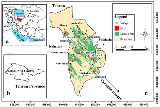
Figure 1.
(a,b) illustrate the study area in Iran and Tehran Province, respectively; (c) the location of the study area (Ghale-Nou County) and the location of field data collection (i.e., ESUs).
2.2. Field Data Measurements and Collections
Based on the map of silage maize farms (Figure 1) and previous years’ map/information including soil texture, soil organic matter, and information provided by farmers at the beginning of the silage maize growing season, a reasonable stratified sampling was used for selecting ESUs with different silage maize varieties and sowing dates to cover as much variability in the study area as possible [29].
Thirty ESUs were identified for field sampling in the study area (Figure 1). LAI and fCover were measured for each ESU using DHP and destructive protocols during the growing season of silage maize from 12 July 2019 to 10 October 2019, with the subsequent calculation of mean values for the two protocols. Biomass measurements of silage maize were also carried out during the field data collection. The time interval between each measurement ranged from 10 to 15 days (6-fold sampling for each ESU), attempting to cover the phenology stages of silage maize (three to four leaves, eight to nine leaves, twelve leaves, flowering, grain formation, and the start of grain-filling stages) (Figure 2). It merits mention that due to delays in the plantation time, the field measurements of 27 July, 1 August, 11 August, and 16 August were carried out in the three-to-four-leaves stage for certain cases. Accordingly, the time of the first sampling was set to three weeks after the plantation on each farm. Therefore, ESUs involved different phenology stages, given the asynchronous cultivation in different farms.
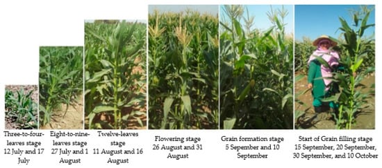
Figure 2.
Field sampling according to the silage maize phenology.
2.2.1. DHP LAI/fCover Measurement
LAI and fCover measurements were carried out in 30 ESUs (6-fold sampling in each ESU) during the growing season of silage maize, simultaneous with S2 data acquisition, with a total of 180 measurements accounting for important phenological stages (Figure 2). The same sampling scheme was used over each ESU, applying the guidelines of the Validation of Land European Remote Sensing Instruments (VALERI) protocol (http://w3.avignon.inra.fr/valeri/ (accessed on 10 May 2019)). The ESUs’ locations were situated far from the farm borders, and the center of the ESU was geo-located using GPS for subsequent matching. To characterize the spatial variability within each ESU, 9 to 12 photos were taken based on the photography plan suggested for homogenous canopies [30]. LAI and fCover were measured using digital hemispherical photographs (DHPs) taken with a Canon 5d Mark II camera equipped with a FC-E8 fisheye lens (Figure 3). For error reduction in the directional gap fraction estimates, the camera was placed at the top of a telescopic tripod to keep the viewing direction downward and the canopy-to-sensor distance constant (~1.5 m) during the growing season, following Claverie et al. [31]. The DHP was processed using CAN-EYE V6.491 (http://www4.paca.inra.fr/can-eye (accessed on 20 October 2019)), to provide estimates of LAI and fCover.

Figure 3.
Samples of DHP taken in ESUs at different phenology stages of silage maize.
2.2.2. Destructive LAI Measurement
Silage maize plant samples were acquired simultaneously with the S2 sensor readings during the growing season. Four plants were destructively harvested from each ESU and the length and width of each leaf were measured manually. The area of each individual leaf was estimated based on the measured length and maximum width of each leaf multiplied by 0.75. LAI was calculated by dividing the total leaf area of each plant by the sampling area; the sampling area was estimated as sample numbers multiplied by row and plant spacing [32]. Canopy cover was also derived using the Ritchie model from Equation (1) [33].
where K is the extinction coefficient assumed to be 0.507643 for maize, based on in situ DHP processing and the Beer–Lambert law [34].
2.2.3. Biomass Measurement
Biomass weight was measured for all samples in all phenology stages of silage maize (4 plants per every 180 samples) via oven-drying. The samples were dried at a temperature of 70 °C for a few days and biomass per unit area was calculated using Equation (2). The calculated biomass in each ESU was used to extract the biophysical biomass using S2 imagery.
2.3. Remote Sensing Data
During the 2019 silage maize growing season, 15 S2 A/B (S2) images (almost all cloud-free) were acquired from 12 July 2019 to 10 October 2019 over the study area (Figure 2). These images were selected based on the phenological information of silage maize crop. The multispectral information of ESA’s S2 satellites covers visible, near-infrared (VNIR), and short-wave infrared (SWIR), and features four bands at 10 m, six bands at 20 m, and three bands at 60 m spatial resolutions. A level-2A image was produced using the Sentinel Application Platform (SNAP) toolbox and a plugin called Sen2Cor.
2.4. Experimental Setup and Validation
To fit MLRA models with S2 spectral reflectance and LAI, fCover, and biomass measurements, field data were collected for model training and validation. The spatial-temporal estimation of fCover, LAI, and biomass was carried out using kernel-based MLRAs: SVR, KRR, RVM, GPR, and VH-GPR. A description of these algorithms with associated references is given in [35]. The hyperparameter-optimized GPR-SA, GPR-TS, GPR-GA, and GPR-PSO were also developed by exploring the capacities of PSO, GA, TS, and SA to optimize the GPR parameters (Figure 4). The performance of these models was compared to the RF and ANN algorithms (multilayer perceptron using back-propagation learning algorithm). The optimal number for trees in RF was obtained, where increases in the number of trees ensured no changes in the estimated error. Also, due to the limited number of output layers, only one hidden layer was adapted, and the Levenberg–Marquardt function was used for ANN training.
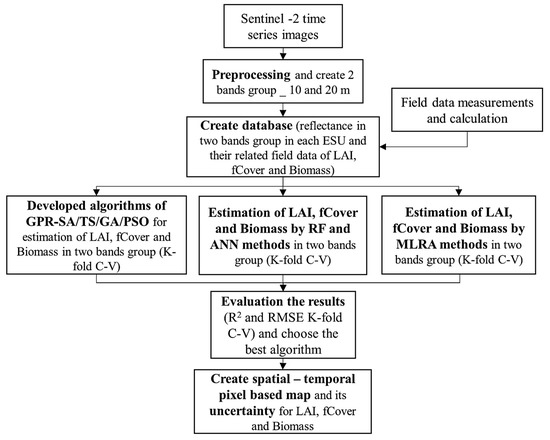
Figure 4.
Flowchart of LAI, fCover, and Biomass estimations using kernel-based MRLA methods, RF, ANN and developed GPR-SA, GPR-TS, GPR-GA and GPR-PSO. ESU, LAI, GPR, SA, TS, GA, PSO, RF, ANN and k-fold C-V in the flowchart are abbreviations of elementary sampling unit (ESU), leaf area index (LAI), gaussian process regression (GPR), simulated annealing (SA), tabu search (TS), genetic algorithm (GA), particle swarm optimization (PSO), random forest (RF), artificial neural network (ANN), and k-fold cross-validation (k-fold C-V).
Regarding the usage of multispectral data into GPR, Verrelst et al. [10] concluded that since the individual bands entered into GPR always lead to superior results, there is no need to calculate vegetation indices before entering into a GPR. That is also the pursued approach here. In the case of hyperspectral data, the effect of multicollinearity starts to degrade the prediction capacity; therefore, applying a dimensionality reduction method, e.g., principal component analysis (PCA), is preferred [36]. Here, field data sampling (i.e., 180 samples) according to two Sentinel configurations (i.e., S2–10 m (4 bands with a spatial resolution of 10 m) and S2–20 m (10 bands with a spatial resolution of 20 m)) were divided into training and validation datasets.
The MLRA methods were evaluated based on a k-fold (10-fold) cross-validation technique, where the dataset was randomly divided into k equal-sized sub-datasets. Here, k-1 sub-datasets were selected as the training dataset and a single k sub-dataset was utilized as the validation dataset for model testing. The cross-validation process was repeated k times, with each k sub-dataset used as a validation dataset only once, and the results of k iterations were combined to produce a single estimation value. The performance or the predictive power of the developed models was evaluated through absolute root-mean-squared error (RMSE) to assess accuracy, and the coefficient of determination (R2) to account for the goodness-of-fit. Subsequently, the best algorithm was selected. To evaluate the MLRA methods by the k-fold cross-validation technique, the average and standard deviation of RMSE and R2 were calculated in cross-validation mode (i.e., RMSE C-V (mean), R2C-V (mean and standard deviation)). Finally, the maps of LAI, fCover, biomass, and their corresponding uncertainty (using standard deviation (SD)), and relative uncertainty (using coefficient of variation (CV; or relative standard deviation/uncertainty, i.e., CV = SD/µ × 100, where µ is the predictive mean [17])) were created using the selected algorithm. The entire workflow was developed in Matlab (2017).
2.5. Hperparameter-Optimized GPR–PSO, GPR-GA, GPR-TS, and GPR-SA Algorithms
The GPR algorithm provides a probabilistic approach for learning generic regression problems with kernels. This model establishes a relation between the input (B-band spectra) x and the output variable (canopy variable) y. Conjugated gradient ascent is typically used for model optimization in the GPR algorithm to estimate hyperparameters θ (, ) (where is a scaling factor (signal scale), is the standard deviation of the (estimated) noise, and a is the length scale per input bands (features), b = 1B) (The length scale describes the smoothness of a function.) by maximizing the negative log marginal likelihood (also called evidence) of the observations. However, this optimization method is heavily dependent on the initial guess and number of iterations and can easily fall into a local optimum due to the use of partial derivatives [27]. To achieve superior performance in optimizing hyperparameters during the training phase, the PSO, GA, TS, and SA optimization algorithms were considered instead of the traditional gradient method (i.e., conjugated gradient ascent method) and proposed GPR-PSO, GPR-GA, GPR-TS, and GPR-SA algorithms. The main advantages of these approaches include convenient procedural treatment, simple and fast implementation, memory function, convergence rate, and quality of optimized designs [26].
In hyperparameter-optimized GPR algorithms, the process of finding the optimal solution (optimal features) can be repeated until the ultimate criterion (higher accuracy in estimating biophysical variables) is met. The marginal probability was considered as the cost function, and the variation in the GPR algorithm parameters (or the meta-heuristic algorithm search space) was tested and set between 0–10, 0–20, and 0–100 in order to develop the proposed algorithms (i.e., GPR-PSO, GPR-GA, GPR-TS, and GPR-SA). Accordingly, the cost function in each iteration was calculated using k-fold cross-validation on training and validation data. The coding of meta-heuristic algorithms was performed in MATLAB (2017).
Steps of the GPR-PSO, GPR-GA, GPR-TS, and GPR-SA Algorithms
In summary, the steps of the proposed GPR-PSO, GPR-GA, GPR-TS, and GPR-SA algorithms are:
Step 1: Choose the initial parameters of the PSO, GA, TS, and SA and GPR models in each hyperparameter-optimized GPR algorithm: PSO = [Npop, max_iteration, w, damping rate, c1, c2]; GA= [Npop, max_iteration, crossover percentage (Pc), mutation percentage (Pm), and mutation rate (Mu)]; TS = [max_iteration, number of neighbors]; SA = [max_iteration, number of neighbors, T0, damping rate]; GPR = [var_min, var_max]. GPR standard algorithms are available at https://github.com/IPL-UV/simpleR (accessed on 20 September 2021).
Step 2: Generate a random initial population and initialize the θ (, ) parameters of GPR algorithm using length scales () = log((max(X) − min(X))/2); SignalPower ( = var(Y) and NoisePower () = SignalPower/4. Construct the composite Cov (or kernel) function by adopting an RBF kernel for signal relations (covSum) with adaptive lengthscale (covSEard), and a diagonal noise covariance matrix (covNoise) based on SimpleR toolbox acquired from [37].
Step 3: Calculate the cost value (or function) using Equation (3),
where K is a kernel function.
Step 4: Update algorithms (with respect to the positions of population in PSO; crossover, mutation, and selection in GA; temperature in SA; and tabu list in TS).
Step 5: Check the convergence criteria: if the stopping criterion is satisfied, terminate the algorithm and return to the optimal hyperparameters of the GPR model; otherwise, return to Step 3. Figure 5 shows the flowchart of GPR-SA (Figure 5a), GPR-TS (Figure 5b), GPR-GA (Figure 5c), and GPR-PSO (Figure 5d) algorithms for modeling biophysical variables.
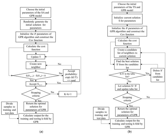
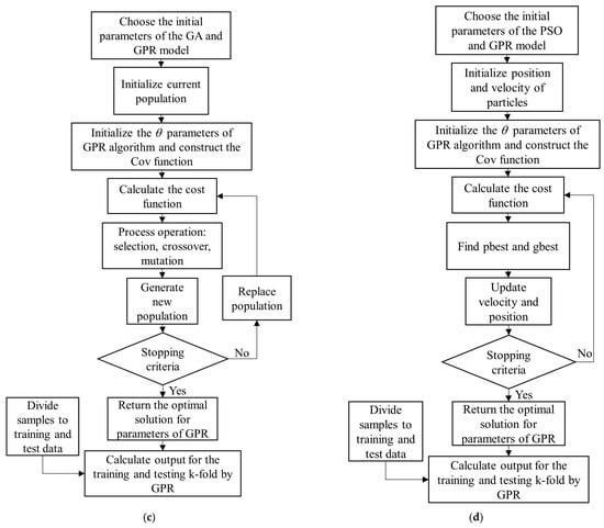
Figure 5.
Flowchart of GPR-SA (a), GPR-TS (b), GPR-GA (c), and GPR-PSO (d) algorithms to model biophysical variables.
3. Results
3.1. Kernel-Based MLRA, RF, ANN, and GPR-PSO, GPR-GA, GPR-TS, and GPR-SA Method Evaluation
The R2 and RMSE estimation results were analyzed using different kernel-based algorithms, as well as the algorithms developed in this study. The results were later compared with RF and ANN as presented in Figure 6a–c. Since a 10-fold cross-validation method was used to validate the algorithms, the corresponding results are also presented as 10-fold mean and standard deviation.
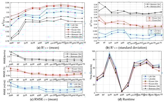
Figure 6.
Assessment of kernel-based MLRAs and developed algorithms compared to RF and ANN in LAI, fCover, and biomass estimation (in 10 and 20 m band groups) by R2 C-V (mean and standard deviation) (a,b), respectively, RMSEC-V (c), and Runtime (d). The RMSE units for LAI, fCover, and biomass were m2/m2, %, and ton/ha, respectively. R2C-V-(µ and σ) and RMSEC-V-(µ) were calculated using µ and σ of results in C-V mode (cross-validation).
Lower R2 C-V standard deviation values signify higher robustness of the algorithm [10]. According to Figure 6, compared with other kernel-based algorithms, GPR-PSO has higher computational accuracy and robustness with higher R2 C-V (mean), lower standard deviation, and lower RMSE C-V in both the 10 m and 20 m band groups of S2. Using this algorithm, it is possible to accurately estimate LAI, fCover, and biomass by combining the four 10 m S-2 bands. Meanwhile, adding bands in the red-edge and SWIR ranges of S2–20 m can improve conformity and accuracy. Among all the algorithms applied to the two S2-band groups, GPR-PSO responded more accurately and robustly in the 20 m S2-band group in estimating LAI, fCover, and biomass with R2 C-V (mean) of 0.917, 0.931 and 0.882, RMSE C-V of 0.627, 0.078, and 1.99, and standard deviation of R2 C-V equal to 0.029, 0.02 and 0.041, respectively. GPR-GA was ranked second for LAI, fCover, and biomass estimation in both band groups with higher accuracy and robustness and lower RMSE. The performance of algorithms in the 20 m band group (including red-edge and SWIR ranges), compared with the 10 m band group, showed an increased R2 C-V (mean), a reduced RMSE and R2C-V (standard deviation), and an improved accuracy in LAI, fCover, and biomass estimation. Only in the 10 m band group did the RF and ANN algorithms, rather than GPR, show more similar R2 values for different k-fold scenarios in the estimation of LAI. However, the computational accuracy of these algorithms (i.e., RF and ANN) was lower than that of kernel-based algorithms in the 10 m and 20 m band groups.
The processing speed is also of the essence for an algorithm to be a good candidate in the operational cycle of estimating biophysical variables over a large area. The runtime (training and validation processing time) calculations presented in Figure 6d are related to a system running Windows 8.1, Intel® Core™ i7-2640M CPU @ 2.80GHz, 4.00 GB RAM in the MATLAB environment. In terms of runtime, the KRR algorithm was the fastest, whereas the SVR algorithm required a longer time for model development in estimating LAI, fCover, and biomass. Only one hyperparameter is involved in the model’s structure through the KRR algorithm, which makes it simpler than other algorithms. Although the RVM algorithm required more runtime than the KRR, accuracy values were similar for both algorithms in the estimation of LAI, fCover, and biomass. GPR was the second fastest algorithm, which, given its high processing speed and accuracy, showed higher computational efficiency in LAI, fCover, and biomass estimation.
Hyperparameter-optimized GPR algorithms developed in this study require more runtime, especially training time, compared with the basic GPR algorithm due to the structure of their optimization method. They are, however, more accurate in LAI, fCover, and biomass estimation.
3.2. Spectral Band Selection for Vegetation Property Retrieval
Another key feature of the GPR algorithm is its ability to assess the importance of bands used in the estimation of biophysical variables thanks to the Automatic Relevance Determination (ARD) covariance function. The ARD provides a separate length scale for each predictor and so allows band relevance determination. Lower values of the length scale (σ) parameter represent higher information content for that band (see also [24]). The bands relevance in model development of LAI, fCover, and biomass variables showed that red-edge and SWIR bands are more effective in the estimation process (Figure 7).
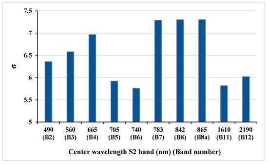
Figure 7.
Significance values (length scale (σ)) of S2 bands in biophysical variable extraction generated by the GPR model: the lower the length scale (σ), the more significant the band.
3.3. Biophysical Variable Retrieval and Pixel-Based Uncertainty Mapping Based on GPR-PSO
In addition to its higher accuracy and robustness, GPR-PSO is significant, given its ability to provide information on the uncertainty of pixel-based estimation of biophysical variables. Considering the higher accuracy and robustness of GPR-PSO in the 20 m S2 band group (Figure 6), this algorithm is used for the mapping of LAI, fCover, and biomass of silage maize, the uncertainty around it (standard deviation), and the coefficient of variation (CV; or relative standard deviation) at the regional level (Figure 8).
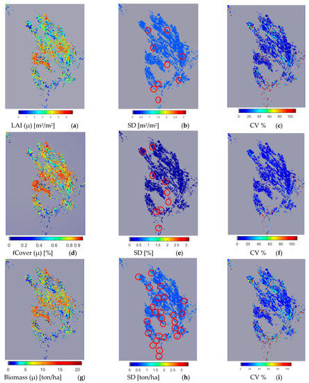
Figure 8.
LAI pixel-based map (a), uncertainty (SD) (b), and CV (c); fCover pixel-based map (d), uncertainty (SD) (e), and CV (f); and Biomass pixel-based map (g), uncertainty (SD) (h), and CV (i) using GPR-PSO in the S2 20 m band group (26 August 2019). Red circles in figures (b,e,h) mark the position of areas with SD > 0.7. See Figure 1 for the geo-information.
S2 image results from 26 August 2019 are presented in Figure 8, marking the flowering of some silage maize fields planted in mid-late June. However, since all farms are not cultivated at the same time, some fields have not yet reached the flowering stage. The spatial variability of LAI, fCover, and biomass values can be seen clearly in these figures. Fields with LAI > 3, fCover > 0.7, and biomass > 7, and areas of 59.5%, 64%, and 44% are located in the central areas of the region, respectively in Figure 8a,d,g. Farms with low LAI are mostly planted at a later time, and those with values close to zero are fallow lands. Figure 8b,e,h present the pixel-based spatial variability of uncertainty (SD) in LAI, fCover, and biomass estimation, respectively. The standard deviation or uncertainty of the majority of farms (for LAI, fCover, and biomass with an area of 96%, 98%, and 71%, respectively) was less than 0.7, while SD values higher than 0.7 were obtained in areas marked by a circle (Figure 8b,e,h) in 4%, 2%, and 29% of the respective fields for LAI, fCover, and biomass (Table 1).

Table 1.
Summarized results of pixel-based map and corresponding uncertainties using GPR-PSO in the S2 20 m band group (26 August 2019) based on Figure 8.
Figure 8c,f,i present the spatial variability of CV for a more significant analysis of uncertainty in LAI, fCover, and biomass estimation and assessment of the GPR-PSO robustness using a pixel-based method. The uncertainty threshold proposed by GCOS is less than 20% [38], while the uncertainty obtained for LAI, fCover, and biomass estimation using this method in the study area was less than 20% in 67%, 84%, and 57% of the fields and less than 30% in 76%, 89%, and 74% of the fields, respectively, indicating the algorithm’s high robustness (Table 1). Only 7% of the croplands led to a CV of more than 100%, which classifies them as fallow lands. Meanwhile, higher CV values were observed in other fields planted at a later time, in which soil was visible in the background alongside plants. Figure 9 and Figure 10 show the pixel-based spatio-temporal variations of the fCover and biomass calculated using the GPR-PSO algorithm in the time series of satellite images. The zoomed images in Figure 9 and Figure 10 show a single experimental field.
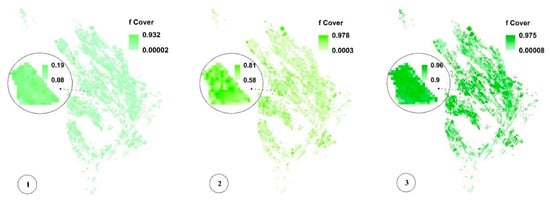
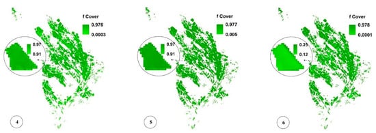
Figure 9.
Pixel-based spatio-temporal variations in fCover (%) calculated using the time series satellite images (taken respectively on 12 July, 27 July, 11 August, 26 August, 5 September, and 20 September, which are only some of the sampling dates). In subimage 6 of Figure 9, the zoomed field is reaped, resulting in decreased fCover values. See Figure 1 for the geo-information.
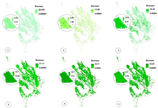
Figure 10.
Pixel-based spatio-temporal variations in Biomass (%) calculated using the time series satellite images (taken respectively on 12 July, 27 July, 11 August, 26 August, 5 September, and 20 September, which are some of the sampling dates). In subimage 6 of Figure 10, the zoomed field is reaped, resulting in decreased Biomass values. See Figure 1 for the geo-information.
4. Discussion
The correlation between the measured LAI, fCover, and biomass values and the recorded reflectance in the 10 and 20 m S2 band groups signifies a nonlinear relationship. Therefore, nonlinear, nonparametric algorithms were used for the estimation of biophysical variables under study. As acknowledged by Verrelst et al. [3,10], linear nonparametric algorithms such as PLSR and PCR cannot estimate such nonlinear relationships. So, the R2 and RMSE estimation results were analyzed using different kernel-based algorithms, as well as the algorithms developed in this study.
Based on the obtained results and according to Verrelst et al. [10], i.e., lower R2 C-V standard deviation values signify higher robustness of the algorithm, GPR-PSO produced superior computational accuracy and robustness over the other kernel-based algorithms, RF and ANN, in both the 10 m and 20 m band groups of S2. Adding red-edge and SWIR ranges in the 20 m band group of S2 led to an increased R2 C-V (mean), a reduced RMSE and R2 C-V (standard deviation), and an improved accuracy of algorithms in LAI, fCover, and biomass estimation. Among all the tested algorithms, GPR-PSO appeared more accurate and robust in the 20 m S2-band group in estimating LAI, fCover, and biomass with R2 C-V (mean) of 0.917, 0.931 and 0.882, RMSE C-V of 0.627, 0.078, and 1.99, and standard deviation of R2 C-V equal to 0.029, 0.02 and 0.041, respectively. Hyperparameter-optimized GPR models developed in this study are more accurate in LAI, fCover, and biomass estimation; however, they require more runtime as compared with the basic GPR algorithm, especially in training time, due to the structure of their optimization method.
The herein-developed GPR models also outperformed the RF and ANN models in accuracy, which makes them better candidates in applied research and large-scale studies. This superiority is largely due to the kernel function used in kernel-based algorithms, especially in GPR, as it estimates nonlinear relations with higher accuracy. The superiority of GPR over other kernel-based algorithms also confirms the higher accuracy of the parameter-tuning method in this algorithm, as opposed to SVR and the absence of optimization in KRR and RVM.
The herein-presented superiority of GPR was also confirmed by Verrelst et al. [10,15], Upreti et al. [39] and Rosso et al. [40], even though the present study investigated the total growth period of silage maize using S2 real data, whereas Verrelst et al. [10,15] used S2 simulated data from Barrax, Spain to investigate various plants by sampling at only one stage of growth. Upreti et al. [39] and Rosso et al. [40] processed S2 real data for retrieving biophysical variables in certain private fields by sampling only some growth stages of wheat and barley. Upreti et al. [39] also introduced kernel-based algorithms, specifically GPR, which outperformed ANN and can be used as an alternative to ANN in operational and applied programs.
Assessing the ARD length scale band relevance in the GPR model development of the targeted biophysical variables revealed that red-edge and SWIR bands are more effective in the estimation process. Similarly, the red edge was selected as among the most sensitive spectral bands to leaf chlorophyll content (LCC), confirmed by Verrelst et al. [24], for assessing band sensitivity of hyperspectral data to biophysical variables such as LCC and LAI by the GPR-based band analysis tool (GPR-BAT). The findings of [24] also indicated that the red edge region, NIR and SWIR contribute to the highest impact of LAI, which was also confirmed by Kira et al. [41]. In our study, this may be a satisfactory reason for why the mentioned bands were selected as the most important bands in variable retrieval of crops using the length scale (σ) parameter of GPR. Therefore, to overcome limitations related to multicollinearity and noisy bands, spectral band selection can be obtained by the length scale (σ) parameter of GPR for optimal biophysical variable retrieval.
Another feature assessed in this study is related to the spatial variability of LAI, fCover, and biomass values. Due to the higher accuracy and robustness of GPR-PSO in the 20 m S2 band group, this algorithm is used for the pixel-based estimation of LAI, fCover, and biomass of silage maize, the uncertainty around it, and the coefficient of variation (Figure 8). The standard deviation or uncertainty (SD) of the majority of farms (for LAI, fCover, and biomass with an area of 96%, 98% and 71%, respectively) was less than 0.7 (Table 1). The relative standard deviation or uncertainty (CV) obtained for LAI, fCover, and biomass estimation using this method in the study area was less than 20% in 67%, 84%, and 57% of the fields and less than 30% in 76%, 89%, and 74% of the fields, respectively; indicating the algorithm’s high robustness (Table 1). The capability of the GPR algorithm for estimating biophysical variables has been evaluated in some comparison studies (e.g., [10,14,15,24,42]), which confirms the results of the present study and the method’s efficiency.
5. Conclusions
The present study proposes the hyperparameter-optimized GPR algorithms for spatio-temporal estimation of biophysical variables using S2 images. The synergetic use of GPR-PSO and red-edge and SWIR bands of S2 enhanced the accuracy of the estimation of LAI, fCover, and biomass at the 20-m spatial resolution. The superiority of the kernel-based algorithms, especially GPR-PSO, over ANN and RF was driven by its kernel-based execution mode and the structure of the PSO meta-heuristic algorithm, which uses both personal flying experience and the experience of other particles to find optimal values. The relative uncertainties over the majority of the study area were below the 20% requirements proposed by GCOS, pointing to the robustness of the GPR-PSO algorithm in estimating LAI, fCover, and biomass. Therefore, considering the accuracy, robustness, and uncertainty associated with the estimation of the agricultural fields’ biophysical variables, it can be concluded that the developed hyperparameter-optimized GPR algorithms applied to S2 imagery make it possible to examine the spatio-temporal variability of LAI, fCover, and biomass in agricultural fields. Finally, toolbox development of hyperparameter-optimized GPR algorithms will allow users to develop accurate and generically applicable biophysical retrieval algorithms; for instance, the optimization algorithms are foreseen to become part of ARTMO’s Machine Learning Regression Algorithm (MLRA) toolbox [43].
Author Contributions
Conceptualization, E.A., A.D.B., J.V., S.P., N.N.S. and S.H.; Data curation, E.A.; Formal analysis, E.A.; Investigation, E.A., A.D.B. and J.V.; Methodology, E.A., A.D.B., J.V. and S.P.; Resources, E.A.; Software, E.A.; Supervision, A.D.B.; Validation, E.A.; Visualization, E.A.; Writing—original draft, E.A.; Writing—review & editing, E.A., A.D.B., J.V., S.P., N.N.S., S.H. and S.S. All authors have read and agreed to the published version of the manuscript.
Funding
This research received no external funding.
Acknowledgments
The authors deeply appreciate the great support from the farmers and organization of agriculture in Ghale-Nou County in this research.
Conflicts of Interest
The authors declare no conflict of interest.
References
- Kross, A.; Mcnairn, H.; Lapen, D.; Sunohara, M.; Champagne, C. Assessment of RapidEye vegetation indices for estimation of leaf area index and biomass in corn and soybean crops. Int. J. Appl. Earth Obs. Geoinf. 2015, 34, 235–248. [Google Scholar] [CrossRef]
- Jin, X.; Yang, G.; Xu, X.; Yang, H.; Feng, H.; Li, Z.; Shen, J.; Zhao, C.; Lan, Y. Combined Multi-Temporal Optical and Radar Parameters for Estimating LAI and Biomass in Winter Wheat Using HJ and RADARSAR-2 Data. Remote Sens. 2015, 7, 13251–13272. [Google Scholar] [CrossRef]
- Verrelst, J.; Camps-valls, G.; Muñoz-marí, J.; Pablo Rivera, J.; Veroustraete, F.; Clevers, J.G.P.W.; Moreno, J. Optical remote sensing and the retrieval of terrestrial vegetation bio-geophysical properties—A review. ISPRS J. Photogramm. Remote Sens. 2015, 108, 273–290. [Google Scholar] [CrossRef]
- Hirose, T.; Ackerly, D.D.; Traw, M.B.; Ramseier, D.; Bazzaz, F.A. CO2 elevation, canopy photosynthesis, and optimal leaf area index. Ecology 1997, 78, 2339–2350. [Google Scholar]
- Mousivand, A.; Menenti, M.; Gorte, B.; Verhoef, W. Multi-temporal, multi-sensor retrieval of terrestrial vegetation properties from spectral—directional radiometric data. Remote Sens. Environ. 2015, 158, 311–330. [Google Scholar] [CrossRef]
- Delegido, J.; Verrelst, J.; Alonso, L.; Moreno, J. Evaluation of Sentinel-2 Red-Edge Bands for Empirical Estimation of Green LAI and Chlorophyll Content. Sensors 2011, 11, 7063–7081. [Google Scholar] [CrossRef]
- Xie, R.; Darvishzadeh, R.; Skidmore, A.K.; Heurich, M.; Holzwarth, S.; Gara, T.W.; Reusen, I. Mapping leaf area index in a mixed temperate forest using Fenix airborne hyperspectral data and Gaussian processes regression. Int. J. Appl. Earth Obs. Geoinf. 2021, 95, 102242. [Google Scholar] [CrossRef]
- Wu, M.; Wu, C.; Huang, W.; Niu, Z.; Wang, C. High-resolution Leaf Area Index estimation from synthetic Landsat data generated by a spatial and temporal data fusion model. Comput. Electron. Agric. 2015, 115, 1–11. [Google Scholar] [CrossRef]
- Houborg, R.; Mccabe, M.F. A hybrid training approach for leaf area index estimation via Cubist and random forests machine-learning. ISPRS J. Photogramm. Remote Sens. 2018, 135, 173–188. [Google Scholar] [CrossRef]
- Verrelst, J.; Pablo Rivera, J.; Veroustraete, F.; Muñoz-Marí, J.; Clevers, J.G.P.W.; Camps-Valls, G.; Moreno, J. Experimental Sentinel-2 LAI estimation using parametric, non-parametric and physical retrieval methods—A comparison. ISPRS J. Photogramm. Remote Sens. 2015, 108, 260–272. [Google Scholar] [CrossRef]
- Chrysafis, I.; Korakis, G.; Kyriazopoulos, A.P.; Mallinis, G. Retrieval of Leaf Area Index Using Sentinel-2 Imagery in a Mixed Mediterranean Forest Area. ISPRS Int. J. Geo-Inf. 2020, 9, 622. [Google Scholar] [CrossRef]
- Estévez, J.; Salinero-Delgado, M.; Berger, K.; Pipia, L.; Rivera-Caicedo, J.P.; Wocher, M.; Reyes-Munoz, P.; Tagliabue, G.; Boschetti, M.; Verrelst, J. Gaussian processes retrieval of crop traits in Google Earth Engine based on Sentinel-2 top-of-atmosphere data. Remote Sens. Environ. 2022, 273, 112958. [Google Scholar] [CrossRef]
- Verrelst, J.; Schaepman, M.E.; Malenovský, Z.; Clevers, J.G.P.W. Effects of woody elements on simulated canopy reflectance: Implications for forest chlorophyll content retrieval. Remote Sens. Environ. 2010, 114, 647–656. [Google Scholar] [CrossRef]
- Verrelst, J.; Alonso, L.; Camps-valls, G.; Delegido, J.; Moreno, J. Retrieval of Vegetation Biophysical Parameters Using Gaussian Process Techniques. IEEE Trans. Geosci. Remote Sens. 2012, 50, 1832–1843. [Google Scholar] [CrossRef]
- Verrelst, J.; Muñoz, J.; Alonso, L.; Delegido, J.; Pablo Rivera, J.; Camps-valls, G.; Moreno, J. Machine learning regression algorithms for biophysical parameter retrieval: Opportunities for Sentinel-2 and -3. Remote Sens. Environ. 2012, 118, 127–139. [Google Scholar] [CrossRef]
- Hastie, T.; Tibshirani, R.; Friedman, J.H. The Elements of Statistical Learning: Data Mining, Inference, and Prediction, 2nd ed.; Springer-Verlag: New York, NY, USA, 2009. [Google Scholar]
- Verrelst, J.; Pablo Rivera, J.; Moreno, J.; Camps-valls, G. Gaussian processes uncertainty estimates in experimental Sentinel-2 LAI and leaf chlorophyll content retrieval. ISPRS J. Photogramm. Remote Sens. 2013, 86, 157–167. [Google Scholar] [CrossRef]
- Müller, K.R.; Mika, S.; Tsuda, K.; Schölkopf, K. An introduction to kernel-based learning algorithms. In Handbook of Neural Network Signal Processing; CRC Press: Boca Raton, FL, USA, 2018; pp. 1–4. [Google Scholar]
- Kiala, Z.Z.Z.S. Modeling Leaf Area Index in a Tropical Grassland Using Multi-Temporal Hyperspectral Data. Master’s Thesis, School of Agricultural, Earth and Environmental Sciences, University of KwaZulu-Natal, Pietermaritzburg, South Africa, 2016. [Google Scholar]
- César de Sá, N.; Baratchi, M.; Hauser, L.T.; van Bodegom, P. Exploring the Impact of Noise on Hybrid Inversion of PROSAIL RTM on Sentinel-2 Data. Remote Sens. 2021, 13, 648. [Google Scholar] [CrossRef]
- Berger, K.; Pablo Rivera Caicedo, J.; Martino, L.; Wocher, M.; Hank, T.; Verrelst, J. A Survey of Active Learning for Quantifying Vegetation Traits from Terrestrial Earth Observation Data. Remote Sens. 2021, 13, 287. [Google Scholar] [CrossRef] [PubMed]
- Pipia, L.; Amin, E.; Belda, S.; Salinero-delgado, M.; Verrelst, J. Green LAI Mapping and Cloud Gap-Filling Using Gaussian Process Regression in Google Earth Engine. Remote Sens. 2021, 13, 403. [Google Scholar] [CrossRef]
- Camps-valls, G.; Verrelst, J.; Muñoz-Marí, J.; Laparra, V.; Mateo-Jiménez, F.; Gómez-Dan, J. A Survey on Gaussian Processes for Earth- Observation Data Analysis. IEEE Geosci. Remote Sens. Mag. 2016, 4, 58–78. [Google Scholar] [CrossRef]
- Verrelst, J.; Pablo Rivera, J.; Gitelson, A.; Delegido, J.; Moreno, J.; Camps-Valls, G. Spectral band selection for vegetation properties retrieval using Gaussian processes regression. Int. J. Appl. Earth Obs. Geoinf. 2016, 52, 554–567. [Google Scholar] [CrossRef]
- Azadbakht, M.; Ashourloo, D.; Aghighi, H.; Radiom, S.; Alimohammadi, A. Wheat leaf rust detection at canopy scale under different LAI levels using machine learning techniques. Comput. Electron. Agric. 2019, 156, 119–128. [Google Scholar] [CrossRef]
- Hong, X.; Ding, Y.; Ren, L.; Chen, L.; Huang, B. A weighted heteroscedastic Gaussian Process Modelling via particle swarm optimization. Chemom. Intell. Lab. Syst. 2018, 172, 129–138. [Google Scholar] [CrossRef]
- Fang, D.; Zhang, X.; Yu, Q.; Jin, T.C.; Tian, L. A novel method for carbon dioxide emission forecasting based on improved Gaussian processes regression. J. Clean. Prod. 2018, 173, 143–150. [Google Scholar] [CrossRef]
- IRIMO. WWW Document. 2019. Available online: www.irimo.ir (accessed on 30 September 2019).
- Akbari, E.; Darvishi Boloorani, A.; Neysani Samany, N.; Hamzeh, S.; Soufizadeh, S.; Pignatti, S. Crop Mapping Using Random Forest and Particle Swarm Optimization based on. Remote Sens. 2020, 12, 1449. [Google Scholar] [CrossRef]
- ESA. SPARC 2004, SPARC Data Acquisition Report; Contract No. 18307/04/NL/FF; ESA: Paris, France, 2005. [Google Scholar]
- Claverie, M.; Demarez, V.; Duchemin, B.; Hagolle, O.; Ducrot, D.; Marais-sicre, C.; Dejoux, J.; Huc, M.; Keravec, P.; Béziat, P.; et al. Maize and sunflower biomass estimation in southwest France using high spatial and temporal resolution remote sensing data. Remote Sens. Environ. 2012, 124, 844–857. [Google Scholar] [CrossRef]
- Xia, T.; Miao, Y.; Wu, D.; Shao, H.; Khosla, R.; Mi, G. Active Optical Sensing of Spring Maize for In-Season Diagnosis of Nitrogen Status Based on Nitrogen Nutrition Index. Remote Sens. 2016, 8, 605. [Google Scholar] [CrossRef]
- Katerji, N.; Campi, P.; Mastrorilli, M. Productivity, evapotranspiration, and water use efficiency of corn and tomato crops simulated by AquaCrop under contrasting water stress conditions in the Mediterranean region. Agric. Water Manag. 2013, 130, 14–26. [Google Scholar] [CrossRef]
- Liu, J.; Pattey, E.; Admiral, S. Assessment of in situ crop LAI measurement using unidirectional view digital photography. Agric. For. Meteorol. 2013, 169, 25–34. [Google Scholar] [CrossRef]
- Verrelst, J.; Malenovský, Z.; Van der Tol, C.; Camps-Valls, G.; Gastellu-Etchegorry, J.P.; Lewis, P.; North, P.; Moreno, J. Quantifying vegetation biophysical variables from imaging spectroscopy data: A review on retrieval methods. Surv. Geophys. 2019, 40, 589–629. [Google Scholar] [CrossRef]
- Pascual-Venteo, A.B.; Portalés, E.; Berger, K.; Tagliabue, G.; Garcia, J.L.; Pérez-Suay, A.; Rivera-Caicedo, J.P.; Verrelst, J. Prototyping crop traits retrieval models for CHIME: Dimensionality reduction strategies applied to PRISMA data. Remote Sens. 2022, 14, 2448. [Google Scholar] [CrossRef] [PubMed]
- Camps-Valls, G.; Gómez-Chova, L.; Muñoz-Marí, J.; Lázaro-Gredilla, M.; Verrelst, J. simpleR: A Simple Educational Matlab Toolbox for Statistical Regression. V3.1.1. 2018. Available online: https://github.com/IPL-UV/simpleR (accessed on 20 September 2021).
- GCOS. Systematic Observation Requirements for Satellite-Based Products for Climate; 2011 Update, Supplemental Details to the Satellite-Based Component of the Implementation Plan for the Global Observing System for Climate in Support of the UNFCCC (2010 update, GCOS-154); World Meteorological Organization: Geneva, Switzerland, 2011; 138p. [Google Scholar]
- Upreti, D.; Huang, W.; Kong, W.; Pascucci, S.; Pignatti, S.; Zhou, X.; Ye, H.; Casa, R. A comparison of hybrid machine learning algorithms for the retrieval of wheat biophysical variables from sentinel-2. Remote Sens. 2019, 11, 481. [Google Scholar] [CrossRef]
- Rosso, P.; Nendel, C.; Gilardi, N.; Udroiu, C.; Chlebowski, F. Processing of remote sensing information to retrieve leaf area index in barley: A comparison of methods. Precis. Agric. 2022, 23, 1449–1472. [Google Scholar] [CrossRef]
- Kira, O.; Nguy-Robertson, A.L.; Arkebauer, T.J.; Linker, R.; Gitelson, A.A. Informative spectral bands for remote green LAI estimation in C3 and C4 crops. Agric. For. Meteorol. 2016, 218–219, 243–249. [Google Scholar] [CrossRef]
- Sinha, S.K.; Padalia, H.; Dasgupta, A.; Verrelst, J.; Rivera, J.P. Estimation of leaf area index using PROSAIL based LUT inversion, MLRA-GPR and empirical models: Case study of tropical deciduous forest plantation, North India. Int. J. Appl. Earth Obs. Geoinf. 2020, 86, 102027. [Google Scholar] [CrossRef] [PubMed]
- Caicedo, J.P.R.; Verrelst, J.; Muñoz-Marí, J.; Moreno, J.; Camps-Valls, G. Toward a semiautomatic machine learning retrieval of biophysical parameters. IEEE J. Sel. Top. Appl. Earth Obs. Remote Sens. 2014, 7, 1249–1259. [Google Scholar] [CrossRef]


Disclaimer/Publisher’s Note: The statements, opinions and data contained in all publications are solely those of the individual author(s) and contributor(s) and not of MDPI and/or the editor(s). MDPI and/or the editor(s) disclaim responsibility for any injury to people or property resulting from any ideas, methods, instructions or products referred to in the content. |
© 2023 by the authors. Licensee MDPI, Basel, Switzerland. This article is an open access article distributed under the terms and conditions of the Creative Commons Attribution (CC BY) license (https://creativecommons.org/licenses/by/4.0/).