Sparse Direct Position Determination Based on TDOA Information in Correlation-Domain

Abstract

The sparse direct position determination (DPD) method requires reconstructing the emitter position with prior knowledge. However, in non-cooperative localization scenarios, it is difficult to reconstruct the transmitted signal with the unknown signal form and propagation model. In this paper, a sparse DPD method based on time-difference-of-arrival (TDOA) information in correlation-domain is proposed. Different from the traditional sparse DPD method, the received signal is converted into correlation-domain, and the proposed dictionary matrix is generated by the quantized delay difference, which solves the pseudo-positioning problem. Compared to the conventional multi-signal classification (MUSIC) method, multi-frequency fusion (MFF) method, and two-step positioning algorithm, the proposed algorithm achieves higher positioning accuracy. The feasibility of the algorithm has been verified by both simulation and real-world measured tests.

1. Introduction

As the positioning-based mobile service attracts more attention, several positioning methods are advancing. In order to overcome the error accumulation effect caused by parameter estimation in traditional time-difference-of-arrival (TDOA) positioning [1], direct position determination (DPD) methods [2,3] have been proposed, which directly establish the likelihood function related to the position according to the signals received by each node, obtaining the positioning result by finding the maximum value of the likelihood function [4].

Studies by Mohammad and other scholars have shown that the DPD method has better positioning performance than the two-step method multipath and low SNR scenarios [5,6]. Direct positioning technology discretizes the space where the radiation source may exist. By dividing the space into a finite number of grids, and establishing a cost function for each grid point according to the maximum likelihood criterion, we can find the grid point with the largest cost function, which is the estimated position of the radiation source. The representative algorithm is Schmidt’s multiple signal classification (MUSIC) based on eigenspace decomposition [7], which uses the orthogonality of the noise and signal subspaces to estimate the spatial spectrum on a grid-by-grid basis. Additionally, as a popular decomposition method, the parallel factor (PARAFAC) [8] analysis is recognized in the DPD field due to its excellent performance at solving the multi-parameter estimation problem in array signal processing. Considering the spectrum estimation, the minimum variance distortionless response (MVDR) method proposed by Weiss [9] is compared with the beamforming method. In view of array signal processing, the spatial scanning beam is generated, and the thermal map will be rendered on the two-dimensional plane to visually display the position distribution probability of the radiation source. Because the traditional DPD method needs to traverse all the grids or generate a full space scanning beam to obtain the likelihood estimation of the emitter position, the positioning result is not optimal under limited measurement data samples and multipath propagation channels. According to the sparsity of the spatial distribution of the radiation source as well as compressed sensing [10], the sparse signal reconstruction algorithm [11] is used to realize the direct localization under small samples and complex multipath conditions.

The sparse signal reconstruction algorithm is based on the compressed sensing algorithm, which breaks through the Nyquist sampling limit, and realizes the sparse reconstruction of signals with fewer observations. A greedy matching pursuit method proposed by Zhang [12] is suitable for emitter localization using the orthogonal matching pursuit (OMP) algorithm [13,14], where the residual satisfies the orthogonal relationship with the selected column atoms in the over-complete dictionary [15]. On the basis of the block sparsity in the dictionary matrices, a block-OMP method, which improves the step of calculating the residual and column atoms in the OMP algorithm, was proposed by Eldar [16]. However, the OMP method performs worse in low signal-to-noise ratio (SNR) cases. Different from the sparse reconstruction method based on the greedy algorithm, the edge likelihood probability function of the original signal pair through the relevance vector machine (RVM) model is based on the sparse Bayesian learning (SBL) algorithm and the expectation–maximization (EM) algorithm, as obtained by Wipf [17]. In lower SNR cases, the SBL-EM method performs better than the matching pursuit method. On this basis, Zhang [18] extends the application of the algorithm under the SBL framework [19,20,21], which inspires the DPD method of sparse emitter sources.

In summary, the traditional two-step positioning method suffers from the issue of error accumulation in the parameter estimation during the initial step. This error propagates into the subsequent steps of the positioning calculation, leading to an overall increase in the positioning error [22,23]. 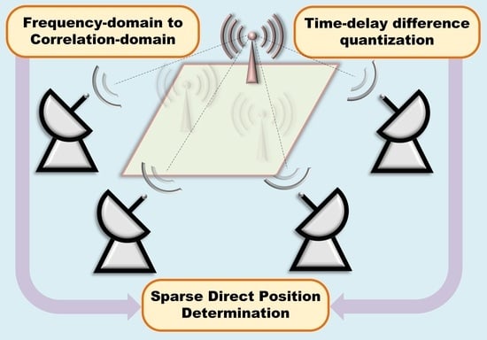Existing DPD methods have their own limitations, such as pseudo-positioning estimation and inadequate robustness [24,25]. Consequently, it becomes challenging to achieve the precise estimation of the radiation source position in a real-world measurement scenario. This paper presents a novel approach, denoted as the correlation-domain-based sparse DPD method, which effectively addresses the problems of error accumulation and pseudo-positioning errors. Moreover, the proposed method demonstrates remarkable robustness in practical scenarios. In Figure 1, we present the flowchart illustrating the research of this paper.

The main contributions of this paper can be summarized as follows:

(1)

The correlation-domain-based sparse DPD model is proposed by transforming the frequency domain received signals into correlation-domain to construct the observation signal for the sparse reconstruction process.

(2)

A modified overcomplete dictionary matrix is constructed based on the quantization-based delay difference. In contrast with the traditional dictionary-generating scheme based on the grid points, the proposed scheme achieves higher accuracy due to classifying the grid points by the time delay difference and solving the pseudo-positioning problem.

(3)

Compared to the multi-signal classification (MUSIC) method, the multi-frequency function fusion (MFF) method [26], and two-step TDOA-Chan positioning method, the proposed algorithm presents more accurate positioning results. Meanwhile, the effectiveness is proved by positioning the results of the real-world measured signals.

2. Sparse DPD Model

Considering a typical TDOA positioning scenario shown in Figure 2, the position coordinates of the radiation source are $\mathbf{P}(x_p,y_p,z_p)$ and the transmitted signal is $s\left(t\right)$. There are L base stations receiving signals, which are located at ${\mathbf{B}}_l(x_{bl},y_{bl},z_{bl}),(l=1,2,\dots ,L)$. The received signal of the l-th base station can be given as follows:

$$x_l\left(t\right)={\beta }_{l}s(t-{\tau }_l)+w_l\left(t\right),$$

(1)

where ${\beta }_l$ is the channel attenuation of the signal transmitted by the emitter to the l-th base station, ${\tau }_l=\Vert \mathbf{P}-{\mathbf{B}}_l\Vert /c$ is the signal transmission delay from the emitter to the l-th base station, $w_l\left(t\right)$ is the stationary zero mean white noise, and c is the speed of light.

According to the time domain form of the received signal in Equation (1), the frequency domain-based discrete form is obtained by performing a uniform sampling on the received signal with a sampling frequency of $f_s$ and the N-point DFT transformation,

$$X_l\left(k\right)={\Gamma }_l\left(k\right)S\left(k\right)+W_l\left(k\right),0\le k\le N-1,$$

(2)

where $S\left(k\right)$ is the DFT transformation of $s\left(t\right)$, $W_l\left(k\right)$ is the DFT transformation of $w_l\left(t\right)$, and ${\Gamma }_l\left(k\right)$ is the complex attenuation of the transmission channel in the frequency domain, which can be expressed as follows:

$${\Gamma }_l\left(k\right)={\alpha }_l\left(k\right){\theta }_l\left(k\right),$$

(3)

where ${\alpha }_l\left(k\right)$ is the amplitude attenuation of each frequency point in the real part, ${\theta }_l\left(k\right)=e^{-j2\pi {\tau }_l{f}_{s}k/N}$ is the phase attenuation caused by the transmission delay in the imaginary part. ${\mathbf{X}}_l$ can be given as follows:

$${\mathbf{X}}_l={\mathbf{\Gamma }}_l\mathbf{S}+{\mathbf{W}}_l={\mathsf{\alpha }}_l{\mathsf{\theta }}_l\mathbf{S}+{\mathbf{W}}_l,$$

(4)

where

$$\begin{array}{c}{\mathbf{X}}_l={[X_l\left(0\right),X_l\left(1\right),\dots ,X_l(N-1)]}^T,\end{array}$$

(5)

$$\begin{array}{c}\mathbf{S}={[S\left(0\right),S\left(1\right),\dots ,S(N-1)]}^T,\end{array}$$

(6)

$$\begin{array}{c}{\mathbf{W}}_l={[W_l\left(0\right),W_l\left(1\right),\dots ,W_l(N-1)]}^T,\end{array}$$

(7)

$$\begin{array}{c}{\mathbf{\Gamma }}_l=\mathrm{diag}{[{\Gamma }_l\left(0\right),{\Gamma }_l\left(1\right),\dots ,{\Gamma }_l(N-1)]}^T,\end{array}$$

(8)

$$\begin{array}{c}{\mathsf{\alpha }}_l=\mathrm{diag}{[{\alpha }_l\left(0\right),{\alpha }_l\left(1\right),\dots ,{\alpha }_l(N-1)]}^T,\end{array}$$

(9)

$$\begin{array}{c}{\mathsf{\theta }}_l=\mathrm{diag}{[1,e^{-j2\pi n_l/N},\dots ,e^{-j2\pi (N-1)n_l/N}]}^T,\end{array}$$

(10)

As the link between the frequency domain and the spatial domain, ${\mathsf{\theta }}_l$ represents the coefficient matrix with the steering vector as the main diagonal element in the frequency domain, and it corresponds to the propagation delay from any position to the l-th base station in the spatial domain. Through the corresponding relationship between the spatial position and the coefficient matrix ${\mathsf{\theta }}_l$, the space is divided into $N_G=N_x\times N_Z$ grids, where the coordinates of the i-th grid point are ${\mathbf{G}}_i(x_{gi},y_{gi},z_{gi})$, then ${\mathsf{\theta }}_l\left({\mathbf{G}}_i\right)$ is obtained.

In the sparse signal reconstruction model, the signal is emitted from all grid points, except one grid contributes the most to the emitted signal, and the other grids contribute little (or even nothing) to the emitted signal. At this time, a contribution function with respect to all grids as independent variables is established; this contribution function is regarded as a sparse signal with only a limited number of non-zero values. The sparse signal is reconstructed, and the position of the non-zero value in the signal is the position of the grid point in the corresponding space.

The first step is to establish the contribution function ${\sigma }_G\left(i\right),(1\le i\le N_G)$ corresponding to all grid points. As the number of signal sources is much less than the number of grid points $(K\ll N_G)$, we can express ${\sigma }_G\left(i\right)$ as ${\sigma }_G\left(i\right)={\widehat{\mathbf{S}}}_i$, expressed as follows:

$$\widehat{\mathbf{S}}=[{\widehat{\mathbf{S}}}_1^T,{\widehat{\mathbf{S}}}_2^T,\dots ,{\widehat{\mathbf{S}}}_{N_G}^T]\in {\mathbb{C}}^{N·N_G},$$

(11)

where ${\widehat{\mathbf{S}}}_i\in {\mathbb{C}}^N$ represents the frequency domain form of the transmitted signal of the grid point. Since the transmitted signals of only a few positions in the space are not zero, $\widehat{\mathbf{S}}$ is in the sparsity space. Based on the idea of compressed sensing, the received signal $\mathbf{X}$ can be denoted as follows:

$$\mathbf{X}=\mathbf{\Phi }\widehat{\mathbf{S}}+\mathbf{W},$$

(12)

where $\mathbf{X}\in {\mathbb{C}}^{N·L}$ represents the observation signal obtained by concatenating the received signals of all base stations, $\mathbf{\Phi }\in {\mathbb{C}}^{N·L\times N·N_G}$ is a super complete dictionary matrix, $\widehat{\mathbf{S}}$ represents a solution vector, $\mathbf{W}\in {\mathbb{C}}^{N·L}$ represents a noise vector, and they can be expressed as follows:

$$\begin{array}{c}\mathbf{X}={[{\mathbf{X}}_1^T,{\mathbf{X}}_2^T,\dots ,{\mathbf{X}}_l^T]}^T,\end{array}$$

(13)

$$\begin{array}{c}\mathbf{\Phi }=\left[\begin{array}{cccc}{\mathbf{\Phi }}_{1,1}& {\mathbf{\Phi }}_{2,1}& \cdots & {\mathbf{\Phi }}_{G_N,1}\\ {\mathbf{\Phi }}_{1,2}& {\mathbf{\Phi }}_{2,2}& \cdots & {\mathbf{\Phi }}_{G_N,2}\\ ⋮& ⋮& \ddots & ⋮\\ {\mathbf{\Phi }}_{1,L}& {\mathbf{\Phi }}_{2,L}& \cdots & {\mathbf{\Phi }}_{G_N,L}\end{array}\right],\end{array}$$

(14)

$$\begin{array}{c}{\mathbf{\Phi }}_{i,l}=\mathrm{diag}{[1,W_N^{n_{i,l}},\dots ,W_N^{(N-1)n_{i,l}}]}^T,\end{array}$$

(15)

where $W_N=e^{-j2\pi /N}$, $n_{i,l}=\frac{\Vert {\mathbf{G}}_i-{\mathbf{B}}_l\Vert f_s}{c}$ represents the number of delay points of the received signal and $f_s$ represents the sampling frequency of the receiver.

Then, the direct positioning problem is converted into the sparse signal reconstruction problem, which can be expressed as an abstract function:

$${\sigma }_G\left(i\right)=SR(\mathbf{X},\mathbf{\Phi }),$$

(16)

where $SR$ represents the sparse reconstruction (SR) algorithm. The input of the algorithm is the received signal $\mathbf{X}$ and the super complete dictionary matrix $\mathbf{\Phi }$. The output of the algorithm is the contribution function ${\sigma }_G\left(i\right)$ of all grid points. The grid point with the largest corresponding function value is the emitter position estimation, expressed as follows:

$${\mathbf{P}}_e=arg\underset{i}{max}\left[{\sigma }_G\left(i\right)\right].$$

(17)

The sparse reconstruction algorithm can be implemented by a variety of sparse reconstruction algorithms, among which, OMP [27] and SBL [28] algorithms are typical ones, which will not be elaborated on in this paper.

3. Sparse DPD Method in Correlation-Domain

In the sparse direct positioning method introduced in the previous section, the signal propagation model is based on the time of arrival (TOA). It is assumed that there is only a propagation delay between the signal received by each base station and the signal sent by the signal source. Moreover, the transmitted signal is reconstructed under the condition of an unknown signal form. These assumptions are difficult to meet in actual scenarios. In this section, a TDOA-DPD method is proposed to transform the frequency domain signal into correlation-domain.

3.1. Construction of the Observation Signal

The TDOA-DPD correlation-domain transformation model is established on the basis of Equation (2). The r-th base station is considered the reference base station, and the reference frequency domain signal $X_r\left(k\right)$ can be obtained by:

$$X_r\left(k\right)={\alpha }_r\left(k\right){\theta }_r\left(k\right)S\left(k\right)+W_r\left(k\right),$$

(18)

where ${\alpha }_r\left(k\right)$ is the reference amplitude attenuation. Except for the frequency domain signal received by the reference base station, $X_l\left(k\right)$ can be represented by the reference frequency domain signal $X_r\left(k\right)$:

$$X_l\left(k\right)=X_r\left(k\right)\frac{X_l\left(k\right)}{X_r\left(k\right)}=X_r\left(k\right)\frac{{\alpha }_l\left(k\right)\left[{\theta }_l\left(k\right)+\frac{W_l\left(k\right)}{{\alpha }_l\left(k\right)S\left(k\right)}\right]}{{\alpha }_r\left(k\right)\left[{\theta }_r\left(k\right)+\frac{W_r\left(k\right)}{{\alpha }_r\left(k\right)S\left(k\right)}\right]},$$

(19)

let ${\xi }_l\left(k\right)e^{\mathrm{j}{\Phi }_l}=\frac{W_l\left(k\right)}{{\alpha }_l\left(k\right)S\left(k\right)}$, where ${\xi }_l\left(k\right)=\left|\frac{W_l\left(k\right)}{{\alpha }_l\left(k\right)S\left(k\right)}\right|$, ${\Phi }_l=arg\left(\frac{W_l\left(k\right)}{{\alpha }_l\left(k\right)S\left(k\right)}\right)$, $l\in \{1,\dots ,L\}$, we have

$$X_l\left(k\right)=X_r\left(k\right)\frac{{\alpha }_l\left(k\right)\left[{\theta }_l\left(k\right)+{\xi }_l\left(k\right)e^{\mathrm{j}{\Phi }_l}\right]}{{\alpha }_r\left(k\right)\left[{\theta }_r\left(k\right)+{\xi }_r\left(k\right)e^{\mathrm{j}{\Phi }_r}\right]}.$$

(20)

When the signal power ${\alpha }_l^2\left(k\right)S^2\left(k\right)$, ${\alpha }_r^2\left(k\right)S^2\left(k\right)$ at the k-th frequency point in the received signal is much greater than the noise power $W_l^2\left(k\right)$, $W_r^2\left(k\right)$,

$$\left|\frac{W_l\left(k\right)}{{\alpha }_l\left(k\right)S\left(k\right)}\right|\ll 1,\left|\frac{W_r\left(k\right)}{{\alpha }_r\left(k\right)S\left(k\right)}\right|\ll 1,$$

(21)

from Equation (21), it can be inferred that ${\xi }_l\left(k\right)\ll \left|{\theta }_l\left(k\right)\right|$, ${\xi }_r\left(k\right)\ll \left|{\theta }_r\left(k\right)\right|$, then $X_l\left(k\right)$ simplifies to:

$$X_l\left(k\right)=X_r\left(k\right)\frac{{\alpha }_l\left(k\right){\theta }_l\left(k\right)}{{\alpha }_r\left(k\right){\theta }_r\left(k\right)}=X_r\left(k\right)\frac{{\alpha }_l\left(k\right)}{{\alpha }_r\left(k\right)}{e}^{-\mathrm{j}2\pi (n_l-n_r)k/N},$$

(22)

let ${\overline{\alpha }}_{l,r}\left(k\right)=\frac{{\alpha }_l\left(k\right)}{{\alpha }_r\left(k\right)}$, ${\overline{\theta }}_{l,r}\left(k\right)=e^{-\mathrm{j}2\pi (n_l-n_r)k/N}$, where $l\in \{1,\dots ,L\}\bigcap \{l\ne r\}$, $X_l\left(k\right)$ is simplified as follows:

$$X_l\left(k\right)=X_r\left(k\right){\overline{\alpha }}_{l,r}\left(k\right){\overline{\theta }}_{l,r}\left(k\right).$$

(23)

Define:

$$Y_{l,r}\left(k\right)=\frac{X_l\left(k\right)X_r^{\ast }\left(k\right)}{{∥X_r\left(k\right)∥}^2}=\frac{X_l\left(k\right)X_r^{\ast }\left(k\right)}{X_r\left(k\right)X_r^{\ast }\left(k\right)}=\frac{X_l\left(k\right)}{X_r\left(k\right)}={\overline{\alpha }}_{l,r}\left(k\right){\overline{\theta }}_{l,r}\left(k\right),$$

(24)

where $X_l\left(k\right)X_r^{\ast }\left(k\right)$ represents the correlation-domain relation of $x_l\left(t\right)$ and $x_r\left(t\right)$. ${\overline{\alpha }}_{l,r}\left(k\right)$ and ${\overline{\theta }}_{l,r}\left(k\right)$, respectively, represent the magnitude and phase of the correlation-domain signals. The matrix form of $Y_{l,r}\left(k\right)$ can be given as follows:

$${\mathbf{Y}}_{l,r}={\left[\begin{array}{cccc}{Y}_{l,r}\left(0\right)& Y_{l,r}\left(1\right)& \cdots & Y_{l,r}(N-1)\end{array}\right]}^{\mathrm{T}}.$$

(25)

Hence, the processing of the received signal from the frequency domain to the correlation-domain is accomplished. The obtained ${\mathbf{Y}}_{l,r}$ is considered the observation signal in the sparse reconstruction model.

3.2. Construction of the Dictionary Matrix

Since the space is divided into $N_G$ grids, ${\mathbf{G}}_i(x_{gi},y_{gi},z_{gi})$ denote the coordinates of the i-th grid point, and ${\Delta }_{l,r}$(i) represents the original time delay difference between the arrival of the i-th grid point at the base station l and the reference base station r:

$${\Delta }_{l,r}\left(i\right)=\frac{\left[∥{\mathbf{G}}_i-{\mathbf{B}}_l∥-∥{\mathbf{G}}_i-{\mathbf{B}}_r∥\right]f_s}{\mathrm{c}},1\le i\le N_G,$$

(26)

where ${\mathbf{B}}_r$ denotes the coordinates of the reference base station and $f_s$ denotes the sample rates. The first step is to find out $min\left\{{\Delta }_{l,r}\left(i\right)\right\}$ and $max\left\{{\Delta }_{l,r}\left(i\right)\right\}$, which are abbreviated as follows: ${\Delta }_{min,l}$, ${\Delta }_{max,l}$. Secondly, we equally divide the interval $[{\Delta }_{min,l},{\Delta }_{max,l}]$ into ${\Lambda }_l$ uniform quantization intervals. Each quantization interval is expressed as $[{\overline{\Delta }}_{l,r}\left({\lambda }_l\right),{\overline{\Delta }}_{l,r}({\lambda }_l+1)]$, ${\lambda }_l=1,2,\dots ,{\Lambda }_l$, and we take the lower bound of each quantization interval as the quantization value. The original delay difference corresponding to all the base stations is quantized to obtain the quantization delay differences of all grid points. Therefore, the quantization delay difference corresponding to the i-th grid point is expressed as follows:

$${\overline{\Delta }}_r\left(i\right)=[{\lambda }_1\left(i\right),{\lambda }_2\left(i\right),\dots ,{\lambda }_L\left(i\right)].$$

(27)

Therefore, the three-dimensional spatial coordinates of the i-th grid point are mapped to a new space composed of the quantization delay difference between the reference base station and other base stations:

$${\mathbf{G}}_i=\left(x_{gi},y_{gi},z_{gi}\right)\to {\overline{\Delta }}_r\left(i\right)=[{\lambda }_1\left(i\right),{\lambda }_2\left(i\right),\dots ,{\lambda }_L\left(i\right)],$$

(28)

where ${\lambda }_l\left(i\right)$ denotes the index of quantization interval, i.e.,

$${\lambda }_l\left(i\right)=arg\underset{\lambda }{min}\left\{\left|{\overline{\Delta }}_{l,r}\left(\lambda \right)-{\Delta }_{l,r}\left(i\right)\right|\right\}.$$

(29)

It is noted that the dimension of ${\overline{\Delta }}_r({\lambda }_1,{\lambda }_2,\dots ,{\lambda }_L)$ is $L-1$, since no delay difference exists with the reference base station r. In other words, the dimension of ${\overline{\Delta }}_r$ can be considered as l, but the value of the r-th dimension remains constant at zero. Thus, the dictionary matrix generated by the quantization delay difference is expressed as follows:

$${\overline{\mathbf{A}}}_{l,r}=\left[\begin{array}{ccccc}1& W_N^{{\overline{\Delta }}_{l,r}\left(1\right)}& W_N^{2{\overline{\Delta }}_{l,r}\left(1\right)}& \cdots & W_N^{(N-1){\overline{\Delta }}_{l,r}\left(1\right)}\\ 1& W_N^{{\overline{\Delta }}_{l,r}\left(2\right)}& W_N^{2{\overline{\Delta }}_{l,r}\left(2\right)}& \cdots & W_N^{(N-1){\overline{\Delta }}_{l,r}\left(2\right)}\\ 1& W_N^{{\overline{\Delta }}_{l,r}\left(3\right)}& W_N^{2{\overline{\Delta }}_{l,r}\left(3\right)}& \cdots & W_N^{(N-1){\overline{\Delta }}_{l,r}\left(3\right)}\\ ⋮& ⋮& ⋮& \ddots & ⋮\\ 1& W_N^{{\overline{\Delta }}_{l,r}(\Lambda )}& W_N^{2{\overline{\Delta }}_{l,r}(\Lambda )}& \cdots & W_N^{(N-1){\overline{\Delta }}_{l,r}(\Lambda )}\end{array}\right],$$

(30)

where $W_N=e^{-\mathrm{j}2\pi /N}$, N denotes the length of the observation signal. Therefore, the sparse reconstruction model is expressed as follows:

$${\mathbf{Y}}_{l,r}={\overline{\mathbf{A}}}_{l,r}{\tilde{\mathbf{Y}}}_{l,r}.$$

(31)

${\tilde{\mathbf{Y}}}_{l,r}$ represents the reconstruction vector i.e.,

$${\tilde{\mathbf{Y}}}_{l,r}={\left[\begin{array}{cccc}{\tilde{Y}}_{l,r}\left(1\right)& {\tilde{Y}}_{l,r}\left(2\right)& \cdots & {\tilde{Y}}_{l,r}(\Lambda )\end{array}\right]}^{\mathrm{T}}.$$

(32)

3.3. Reconstruction of the Source Location

Since ${\tilde{\mathbf{Y}}}_{l,r}$ is sparse, the position of its non-zero value corresponds to the quantization interval index ${\tilde{\lambda }}_l$. After the $(L-1)$ times sparse reconstruction of the $(L-1)$ correlation-domain signals, one has

$$\tilde{\mathsf{\lambda }}=\left[\begin{array}{cccc}{\tilde{\lambda }}_1& {\tilde{\lambda }}_2& \cdots & {\tilde{\lambda }}_L\end{array}\right],$$

(33)

Reviewing the mapping relation in Equation (28), it is expected that the three-dimensional coordinates of the grid points can be inversely mapped according to the vector $\tilde{\mathbf{\lambda }}$. Thus, the following mapping relationship is considered:

$${\overline{\Delta }}_r=[{\tilde{\lambda }}_1,{\tilde{\lambda }}_2,\cdots ,{\tilde{\lambda }}_L]\to {\mathbf{G}}_i=\left(x_{gi},y_{gi},z_{gi}\right).$$

(34)

The method adopted here is to map each ${\tilde{\lambda }}_l$ separately and perform $(L-1)$ times mapping operations in total. The reason is that the mapping in Equation (28) is likely not surjective. It is likely that the corresponding ${\mathbf{G}}_i$ cannot be found according to the obtained $\tilde{\mathsf{\lambda }}$. However, it is assumed that ${\mathbf{G}}_i\to {\lambda }_l$ is a surjective, i.e., the time delay difference of all grid points after quantization for a certain base station can always be completely traversed, and the corresponding ${\mathbf{G}}_i$ can be found according to ${\tilde{\lambda }}_l$ (usually not unique). This assumption holds only if the delay difference quantization interval is large enough to ensure that each mapping is surjective. The specific steps are as follows:

(1)

When $l=1$, we find that all ${\overline{\Delta }}_r\left(i\right)$ meet the following condition: ${\lambda }_1\left(i\right)={\tilde{\lambda }}_1$, then we record the index of the grid point as $i_1$, and assign ${\tilde{\mathbf{Y}}}_{1,r}\left({\tilde{\lambda }}_1\right)$ to ${\sigma }_G\left(i_1\right)$, which indicates the likelihood function of the grid point.

(2)

When $l=2$, we find that all ${\overline{\Delta }}_r\left(i\right)$ meet the following condition: ${\lambda }_2\left(i\right)={\tilde{\lambda }}_2$, then we record the index of the grid point as $i_2$, assign ${\tilde{\mathbf{Y}}}_{2,r}\left({\tilde{\lambda }}_2\right)$ to ${\sigma }_G\left(i_2\right)$, and accumulate with ${\sigma }_G\left(i_1\right)$.

(3)

When $l=3,4,\dots ,L$, by analogy, the ${\sigma }_G$ function obtained each time is accumulated with the previous one, and the final ${\sigma }_G$ function is the likelihood function of all grid points.

Since the grid point coordinates ${\mathbf{G}}_i$ mapped by $\tilde{\mathsf{\lambda }}$ exist in each value record $i_1,i_2,\dots ,i_L$ after $(L-1)$ times accumulation, the grid point with the largest likelihood function value represents the grid point coordinates mapped by $\tilde{\mathsf{\lambda }}$. Thus, the source position estimation ${\mathbf{P}}_e$ can be expressed as follows:

$${\mathbf{P}}_e=\left\{{\mathbf{G}}_q\left|q=arg\underset{i}{max}\left[{\sigma }_G\left(i\right)\right]\right.\right\}$$

(35)

Through improvements, the original single sparse reconstruction is changed to multi-dictionary joint sparse reconstruction for each correlation-domain signal, and $(L-1)$ quantized delay difference matrices are used as dictionary matrices to obtain $(L-1)$ reconstructed vectors. By searching the index of each grid point’s delay difference in the corresponding quantized delay difference dictionary, the reconstructed vector component value of the grid point, i.e., the likelihood function, is determined, and the likelihood functions of all grid points are reconstructed.

The proposed algorithm can be summarized as in Algorithm 1.

Algorithm 1: Sparse TDOA-DPD Algorithm

4. Simulation

Simulation 1: The horizontal–vertical coordinate range of the task area was [0 m, 200 m] divided into a 4 m × 4 m grid. There were four base stations distributed in the four corners of the task area. The location of the radiation source was fixed (40 m, 60 m). The positioning was performed 100 times. The signals transmitted by each base station were different complex Gaussian signals, with a signal length of 32 and an SNR of 10 dB. The SBL sparse reconstruction algorithm was adopted based on the TDOA-DPD model; the positioning results are shown in Figure 3. In this figure, it is evident that the peak value of the likelihood function precisely corresponds to the actual position of the radiation source.

Simulation 2: The comparison of positioning results before and after the time delay quantization is shown in Figure 4. Figure 4a shows several pseudo-positioning results due to the absence of the time delay quantization step. Figure 4b shows the correct positioning result with time delay quantization. Looking at the comparison via the two subfigures, it can be concluded that the quantized delay difference dictionary effectively eliminates the pseudo-positioning problem.

Simulation 3: The source position was randomly generated in the task area, and the positioning was performed 100 times. The other parameters are the same as those in simulation 1. The RMSE vs. SNR curves are investigated and compared with other positioning methods, as shown in Figure 5.

The mean absolute error (MAE) and the root mean square error (RMSE) are given as follows:

$$MAE=\frac{1}{N_m}\sum _{i=1}^{N_m}\parallel {\widehat{\mathbf{p}}}_i-\mathbf{p}\parallel$$

(36)

$$RMSE=\sqrt{\frac{1}{N_m}{\displaystyle \sum _{i=1}^{N_m}}{\parallel {\widehat{\mathbf{p}}}_i-\mathbf{p}\parallel }^2}$$

(37)

where $N_m$ is the simulation time under the same SNR, ${\widehat{\mathbf{p}}}_i$ is the i-th estimation to the emitter source, and $\mathbf{p}$ is the real position of the source.

According to Figure 5, the proposed method achieves higher accuracy compared to other positioning methods. In situations with high SNR, all four methods exhibit similar performance. However, at low SNR levels, both the TDOA-Chan and DPD-DET methods demonstrate inferior performance compared to the other two methods. Based on the color bars in Figure 6, it is evident that the proposed method outperforms the other methods in a variety of metrics, including the 25th percentile error, median error, 75th percentile error, and mean absolute error.

5. Real-World Measured Tests

In the real-world measured scenario, the specific parameters of the measured data are shown in

Table 1. Parameters of real-world measured data.

Parameter Name	Value	Parameter Name	Value
Modulation Mode	QPSK	Sample Rate	125 MHz
Symbol Rate	25 MSPS	Signal Length	4096
Center Frequency	726 MHz	Number of Sources	1
Radiation Power	15 dBm	Number of Base Stations	4

. The real emitter and the node equipment are, respectively, illustrated in Figure 7. On the left side, the actual picture of the receiver node and the emitter source are presented, while on the right, the real scenario is displayed.

The real-world measured signals collected within 30 seconds were located using a traditional two-step TDOA-Chan positioning method; the results based on traditional two-step TDOA-Chan positioning are shown in Figure 8a. Next, the proposed sparse DPD positioning method was used to locate the same original data, Figure 8b exhibits the thermal map of the positioning results. Figure 9 shows the positioning error CDF curve of the measured signal.

In Figure 8a, the scatter points of the positioning results are located near the emitter position, and the yellow stars are symbols of the nodes. In Figure 8b, the color map visually represents the likelihood function, which corresponds to the probability distribution of the emitter source’s location. In Figure 9, it is demonstrated that the proposed method exhibits the minimum error compared to other positioning methods, and the DPD-DET method has the worst performance in real-world measured tests. By sorting the positioning error values in ascending order, we were able to identify the error corresponding to the 90th percentile; thus, we achieved the desired error measurement at the 90% confidence level. At the 90% confidence level, the proposed method obtains the highest accuracy, which is less than the 10-meter error. In

Table 2. Positioning errors of real-world measured data.

	TDOA-Chan	DPD-DET	DPD-MFF	Proposed Method
25 percentile error	4.9802 m	5.9870 m	4.7013 m	3.3741 m
Median error	6.5835 m	13.3595 m	7.5158 m	4.9038 m
75th percentile error	8.8934 m	18.5046 m	9.6559 m	8.4570 m
Mean absolute error	7.2088 m	16.5353 m	7.0809 m	5.1925 m
RMSE	7.8456 m	22.3492 m	7.9656 m	5.9784 m

, five metrics of the measured positioning error are listed, including the 25th percentile error, median error, 75th percentile error, and mean absolute error. The proposed method gains the highest accuracy compared to the other methods. Relative to its performance in simulation 3, the proposed method shows its robustness for outperforming other methods both in simulation and the real-world measured test.

6. Conclusions

In this paper, a sparse DPD method is proposed that is based on TDOA information in correlation-domain. The main process involves converting the signal from the frequency domain to the correlation-domain and the construction of the quantized delay difference dictionary matrix. This study has demonstrated the effectiveness of the proposed method in mitigating the issues of error accumulation and pseudo-positioning errors encountered in traditional methods. Through extensive experimentation based on the real-world measured tests and analysis, we have shown that the correlation-domain-based sparse DPD method significantly improves the accuracy and robustness of radiation source localization. Moreover, the proposed method exhibits remarkable performance in practical scenarios, highlighting its potential for real-world applications.

Future work will aim to expand the algorithm’s scope to more universal positioning scenarios, including the localization and tracking of signals employing complicated modulation techniques within complex electromagnetic environments.

7. Discussion

While the research in this paper primarily concentrates on static radiation source localization, it is worth noting that the field of positioning and tracking dynamic radiation targets is gaining more attention. Therefore, it is crucial to conduct further research to assess the applicability of the proposed algorithm in mobile multi-target localization scenarios.

Overall, our study contributes to the advancement of radiation source positioning methods. The proposed algorithm holds great promise for improving the accuracy and reliability of radiation source localization systems, ultimately enhancing the effectiveness in various domains, including illegal aerial vehicle monitoring, interference source localization, and emergency responses.