Information Leakage in Deep Learning-Based Hyperspectral Image Classification: A Survey

Abstract

In deep learning-based hyperspectral remote sensing image classification tasks, random sampling strategies are typically used to train model parameters for testing and evaluation. However, this approach leads to strong spatial autocorrelation between the training set samples and the surrounding test set samples, and some unlabeled test set data directly participate in the training of the network. This leaked information makes the model overly optimistic. Models trained under these conditions tend to overfit to a single dataset, which limits the range of practical applications. This paper analyzes the causes and effects of information leakage and summarizes the methods from existing models to mitigate the effects of information leakage. Specifically, this paper states the main issues in this area, where the issue of information leakage is addressed in detail. Second, some algorithms and related models used to mitigate information leakage are categorized, including reducing the number of training samples, using spatially disjoint sampling strategies, few-shot learning, and unsupervised learning. These models and methods are classified according to the sample-related phase and the feature extraction phase. Finally, several representative hyperspectral image classification models experiments are conducted on the common datasets and their effectiveness in mitigating information leakage is analyzed.

1. Introduction

The analysis and processing of remote sensing data is one of the common methods of observing the Earth’s surface. With the rapid development of optical sensors, researchers are gradually focusing on spectral information hidden beyond the visible light band. Hyperspectral imaging is used to image tens or even hundreds of narrow spectral bands in a fixed area by remote sensing. Hyperspectral images (HSIs) can be viewed as 3D images, where each pixel contains all the band information acquired at that point, providing a richer and more-refined spectral feature for the ground-based object. Therefore, hyperspectral data processing has been widely used in numerous fields, such as precision agriculture [1,2,3], marine resource exploration and mapping [4], water quality analysis [5], military target detection [6], mineral exploration [7], and medical detection and diagnosis [8]. However, the same ground-based object may have different spectral properties due to atmospheric, temperature, spatial resolution, and other effects, and the spectral properties of different ground-based objects may be similar. This leads to salt-and-pepper noise and over-smoothing in the recognition task, which increases the challenges of object recognition. It is difficult to manually extract effective deep features from the large amount of nonlinear redundant spectral information. Therefore, traditional hyperspectral image (HSI) classification methods may not be able to distinguish subtle gaps between different classes of ground-based objects.

With the continuous development of machine learning, learning-based algorithms have been introduced to the field of HSI classification with great results. Due to the abundant spectral information of HSIs, in the early use of shallow machine learning algorithms, researchers focused on high-dimensional spectral information and related feature extraction models, such as Support Vector Machine (SVM) [9]. On this basis, Li et al. [10] proposed the SVM model based on multiple cores. Liu et al. [11] proposed the SVM model based on nonparallelism. In addition, some machine learning-related algorithms such as random forest [12], polynomial logical regression [13,14], and random subspace method [15,16,17] have also been introduced into the field of HSI classification. However, the spatial feature extraction capabilities of traditional machine learning still have the potential to be optimized.

In recent years, with the development of graphics processing unit (GPU) computing performance, deep learning has emerged and been applied to various fields. It has changed the processing methods of remote sensing data, such as object detection [18,19], super-resolution [20], and change detection [21]. Deep learning-based HSI classification has become a research hot spot in this field. Chen et al. [22] first introduced deep learning into the classification task of HSI and combined it with principal component analysis (PCA). Specifically, the first principal component of the neighborhood is first extracted to obtain the spatial information, which is then flattened into a one-dimensional vector and fed into a stacked autoencoder (SAE). Finally, classification is performed by logistic regression. The results demonstrated advanced performance at the time and revealed the great potential of deep learning models for HSI classification. Since then, refs. [23,24,25] retained three principal components, borrowed from RGB image processing methods, and combined with convolutional neural network (CNN) to further utilize spatial information.

After 2D convolutional neural networks (2D-CNN), 3D convolutional neural networks (3D-CNN) are also widely used in HSI classification tasks [26]. Roy et al. [27] combined residual network and attention mechanism on this basis, and achieved significantly better classification results than 2D-CNN. While achieving better performance, limited labeled samples of HSI data should also be considered. Refs. [28,29] used few-shot learning (FSL) to improve classification accuracy with limited available samples. Compared to traditional machine learning methods such as SVM, deep learning-based HSI classification algorithms can extract deep features in an end-to-end network and overcome problems such as salt-and-pepper noise. While deep learning has achieved some state-of-the-art results in the field of HSI classification, it still faces two challenges:

• HSI data is high-dimensional, and labeling cost is high. Therefore, fewer training samples are commonly used in training, which will bring difficulties to feature extraction, affect model performance, and cause the Hughes phenomenon [30];
• When HSI data is used to train the network by using random sampling strategy and the input is patch format, some information of the test set will be leaked. This affects the generalization ability of the model [31], making the model only learn the distribution of one domain.

These two challenges make deep learning-based HSI classification limited in practical applications. An ideal practical model is one that can be trained on one dataset, and then perform satisfactorily when tested on another given dataset.

Most deep learning algorithms use random sampling to train and test on a single HSI, ignoring the information leakage problem in the process. If the training set is selected using a random sampling strategy, the information leakage becomes more severe as the number of training samples increases. This leads to overly optimistic accuracy, poor generalization ability, and limited practical applications. Molinier et al. [31] found that when more than 10% training samples of 3 × 3 patches were used, over 50% of the test pixels were directly involved in the training stage. The increase of patch size will also increase the overlap area of samples, which will further affect the heterogeneity of the test set and training set [32].

Table 1. The sources, problems, and mitigation methods for information leakage of HSI classification.

Source	Problem	Mitigation Methods
Excessively similar samples	Overly optimistic classification performance	Spatially disjoint sampling strategies
Overlap between samples	Reduced generalization ability	Fewer training samples
Training samples contain test information	Practical applications are limited	Extraction of general features

summarizes the sources, problems, and mitigation methods for information leakage. In order to alleviate this effect, some different sampling strategies have been proposed in addition to the random sampling mode [33,34]. From a feature extraction perspective, some cross-domain modular learning models such as few-shot learning can also alleviate the impact of information leakage.

To the best of our knowledge, few quantitative evaluation methods have been used to measure the impact of information leakage in the field of hyperspectral remote sensing image classification. Qu et al. [35] divided the HSI dataset into training area, leakage area, validation area, and test area. The training area and test area are used to evaluate the model performance, and the leakage area is used to evaluate the degree of information leakage. It is more common to qualitatively observe the impact of information leakage by comparing the gap between different sampling methods [36]. In addition, the number of test set pixels directly involved in model training can be calculated, as well as the similarity between training set samples and nearby samples. These indicators reflect the degree of information leakage and the strength of generalization ability to some extent.

The main work of this paper can be divided into three aspects:

1.

Some of the existing problems in the field of deep learning-based HSI classification are summarized. The information leakage problem caused by the introduction of spatial information is introduced in detail;

2.

Depending on the cause of information leakage, this paper discusses some mitigation methods in the field of deep learning-based HSI classification. Based on this, we explore the performance of some existing related models and algorithms on the information leakage problem. All the mentioned methods are summarized in terms of sample related phase and feature extraction phase;

3.

This paper experimentally compares the effectiveness of some models and algorithms for mitigating information leakage.

2. Methods

2.1. Problems and Challenges

With the development of machine learning, scholars have gradually realized the significant advantages of deep learning-based algorithms. These methods not only offer better classification performance, but also overcome numerous challenges faced by traditional algorithms [37]. While various deep learning-based algorithms have been introduced for HSI classification, several challenges have emerged. These problems can be divided into two aspects, namely some difficulties in deep learning algorithms and challenges that arise when HSI classification tasks are combined with deep learning models. The former includes huge computation and time cost, vanishing gradient and “black box” characteristics, etc., which will not be described in this paper. The latter are caused by the characteristics of the HSI data. This paper summarizes the challenges faced by deep learning-based HSI classification models into two categories based on their causes. The first problem is the limited number of training samples, and the second problem is information leakage.

2.1.1. Limited Training Samples

The HSI classification task is a pixel-wise classification task. The label annotation process is a pixel-by-pixel annotation of the HSI data collected in a certain region. Compared to the process for RGB images, HSIs pose three significant challenges. First, unlike RGB image classification tasks that use the entire image as a sample, pixel-wise training samples of HSIs are usually difficult to obtain due to the time-consuming nature of manual labeling. Second, the spatial resolution of HSIs is lower than that of RGB remote sensing images, which is caused by the mutual restriction between spatial and spectral resolution of remote sensing images. Low spatial resolution results in the loss of texture and additional details of the ground-based object, further increasing the difficulty of HSI classification. Finally, HSIs are affected by factors such as atmosphere, temperature, humidity, etc., at the time of data acquisition. Spectra of various objects may vary to varying degrees, resulting in the effect of different spectra of the same object or different objects with the same spectrum. In addition, due to the different imaging equipment used in the data acquisition process of different HSI datasets, the spatial resolution, spectral resolution, spectral range, imaging time, and imaging area are also different. These hardware conditions result in different spectral signatures for the same ground-based object. Therefore, when performing classification tasks on HSIs from different regions, it is necessary to label and train separately. Even unsupervised learning inevitably requires some training samples for fine-tuning [38,39]. However, most HSI classification algorithms still aim to improve classification performance on a single image. This is one of the triggers for subsequent information leakage and overfitting.

In this context, deep learning models that support training with few samples need to be considered for HSI classification tasks. Recently, many scholars have focused on how to improve classification accuracy in the case of few samples. However, the Hughes effect occurs when the number of training samples is insufficient, that is, the classification accuracy first increases and then decreases as the dimensionality of the input features increases. Some researchers have noticed this problem and have effectively mitigated the Hughes effect by various ways of data dimensionality reduction [40,41,42]. In addition, in the field of HSI classification, some deep learning-related algorithms and models have achieved great results with few training samples, such as data augmentation [43], FSL [29], active learning [44].

2.1.2. Information Leakage

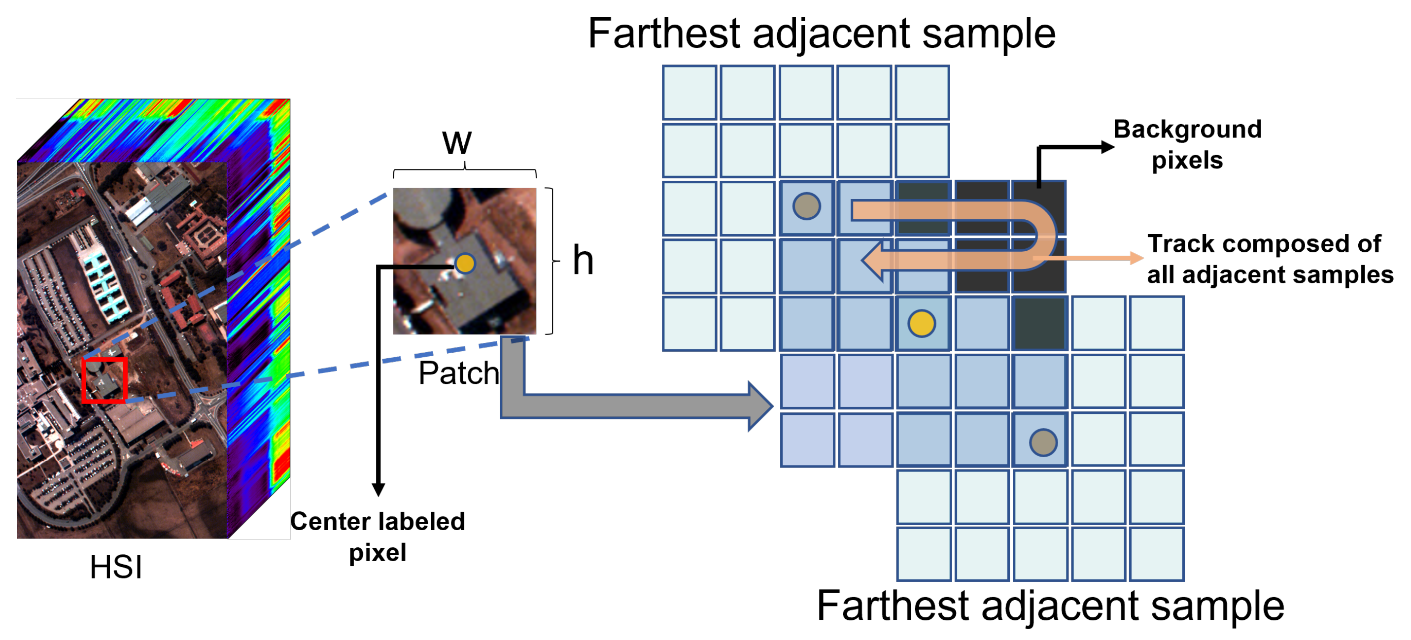
Since the training set and test set of most deep learning-based HSI classification models originate from the same image. Random sampling will make the training samples more evenly distributed in each spatial location of the entire HSI map. The remaining nearby pixels constitute the test set. This pixel-wise distance results in the test sample being able to find nearly identical training samples in its vicinity. Constructing the input with image patches is a common way to introduce spatial information. However, this approach not only increases the similarity between samples, but also exposes some test samples during network training. Therefore, there is a strong spatial correlation between the training set and the test set under the random sampling strategy, which will threaten the assumption of sample independence [33] and cause information leakage. The information leakage problem mentioned in this paper belongs to the field of remote sensing classification. Specifically, this problem refers to exposing some information of the test set to the training process, resulting in overly optimistic model results. As shown in Figure 1, the input samples of most deep learning models are patches of h × w × b, where h × w represents the neighborhood range of the sample and b represents the band dimension or the number of principal components retained after dimension reduction using PCA. The sources of information leakage can be mainly divided into two aspects:

First, the pixel values derived from HSIs consist of a finite number of spectral responses of different ground-based objects. This results in a tight relation between similarity and distance; namely, training samples and their nearby test samples are excessively similar. In early studies of land cover mapping via remote sensing images, researchers generally used the spatial location information of the image as a feature. For example, the 1-Nearest Neighbor algorithm thus leads the model to learn correlations between samples and the target spatial distribution, rather than between classes. This problem was first noticed by Friedl et al. [45], who attributed this strong clustering of data to spatial autocorrelation [46]. That is, when supervised learning performs a random sampling strategy to obtain the training set, part of the test samples will have strong spatial dependence with the training samples. The samples used for testing can always find the training samples in their vicinity, leading to an optimistic evaluation of accuracy. Zhen et al. [47] conducted experiments based on object classification through two different sampling strategies to investigate the influence of sampling on classification results. Later, the HSI classification task based on deep learning is also faced with this problem [34]. The First Law of Geography states, “everything is related to everything else, but near things are more related than distant things”. Most ground-based objects in the same class of HSI data are distributed together and have strong spatial autocorrelation. This correlation is different from previous mapping works. HSIs have abundant spectral information that can be used for classification, but if only spectral information is used, the situation of the same object with different spectra will lead to severe salt-and-pepper noise. Therefore, spatial information also needs to be considered in the algorithm. As shown in Figure 1a, the deep learning model commonly extracts the spatial feature in the form of patch [24,26]. This form of input leads to overlap between samples. In the case of random sampling, the neighborhood cube of a pixel in the training set will be extremely similar to the neighborhood cube of a pixel in the nearby test set. The similarity would also threaten the independence of the sample and obtain overly optimistic classification performance. Correspondingly, the classification accuracy under the spatially disjoint sampling strategy shows varying degrees of decline [48].

Second, the spectral information of the test set pixels is directly trained into the network [49]. Figure 1b shows that when the training set is selected by random sampling, some pixels of the test set will be included in the patches of the training samples due to the introduction of spatial information. It is experimentally verified that as the input patch size continues to increase, the test samples not exposed to network training become fewer [31]. Therefore, in some studies, appropriately increasing the neighborhood size improves the classification accuracy with random sampling strategy [43,50]. It is worth noting that the test pixels directly involved in training are only used as neighborhood information. This information cannot affect the labels of the training samples. In other words, the labels of these leaked test pixels are not fed into the network and they do not participate in backpropagation.

Both sources of information leakage mentioned above are related to spatial information. In the field of HSI classification, if the features are only extracted from the spectral information to construct a classifier and the spatial context information is not explored, each sample is a pixel of a one-dimensional vector and there is no overlap between the test set and the training sets. While this can strictly avoid the test set participating in the network training directly, it typically produces severe salt-and-pepper noise. After adding spatial information, a significant improvement in classification accuracy can be observed [51]. Therefore, it is necessary to introduce spatial context information. For a training sample, the ideal spatial information extraction should satisfy two points. First, it can explore the clustering properties of similar ground-based objects. Second, it avoids introducing test sample information or learning some unique distributional shape rule for a single dataset. The former, according to The First Law of Geography, aims to learn the commonality of the distribution of ground-based objects. The latter is a reference to The Second Law of Geography to mitigate overfitting to a single dataset. However, due to the black-box nature of deep learning, it is difficult to simultaneously satisfy the above two conditions when extracting spatial information. Therefore, it is difficult to distinguish whether this optimistic classification accuracy is caused by the effective spectral spatial features or by information leakage [34].

From related works in remote sensing and mapping to the current research on HSI classification techniques, a growing number of scholars have begun to focus on the study of spatial autocorrelation, sampling strategies, sample overlap, overfitting, and other information leakage-related directions. Figure 2 summarizes some related works and points out the sampling strategies and feature extraction models used in these works. In addition to the aforementioned models for dealing with information leakage, this paper analyzes the effectiveness of some existing models and algorithms for mitigating information leakage in terms of sample related phase and feature extraction phase. In order to clearly illustrate the impact of information leakage, datasets with the same spatial resolution, spectral resolution, and ground-based objects collected in similar atmospheric environments are referred to as homogeneous datasets in this paper. Then based on this, the phenomenon of overfitting is classified into two types, namely overfitting within a single dataset and overfitting between datasets. The first one refers to the mapping process where the network overfits the labels in the training set and performs poorly for the test set in the same dataset. The second is that when using homogeneous datasets, the model performs well on a single dataset and poorly on the other homogeneous datasets. The generalization ability of the model should also be classified into the generalization ability of the above two cases. Data leakage leading to overfitting and low generalization generally refers to the second case.

2.2. Overfitting between Datasets Caused by Information Leakage

When the number of samples is relatively sufficient, randomly sampled training samples are chosen to uniformly cover the entire HSI. All spectral variations of almost every object in the dataset are learned. However, in practical applications, there is a considerable number of different variants of the same class of ground-based objects that have not been learned. Therefore, during training process, a model should focus more on general features of objects of the same class, rather than fitting specific features of a single dataset. As shown in Figure 3, it is assumed that a given type of ground-based object in the HSI dataset contains multiple cases of different spectrum (different color boxes indicate different types of spectral variation areas). If the training set is chosen by random sampling, it will be relatively easier to learn all these cases. When the trained model is used on the homogeneous dataset, the ability to fit different spectral variability features is reduced. To some extent, information leakage can cause the knowledge acquired by a deep learning model to be biased towards some features of a particular dataset, which affects the generalization ability of the model. Namely, the trained model may perform poorly when tested on other datasets of the same class. To the best of our knowledge, there are no such labeled publicly available homogeneous datasets that contain multiple HSIs. However, it is a common practical application scenario that the same hyperspectral remote sensing imaging device acquires multiple HSIs of a certain region. Improving the generalization performance of models for homogeneous datasets is of practical interest. In recent years, there have also been works on using trained models to directly classify with different types of datasets [52]. These models typically require some preprocessing of the samples to extract generalization features across different datasets.

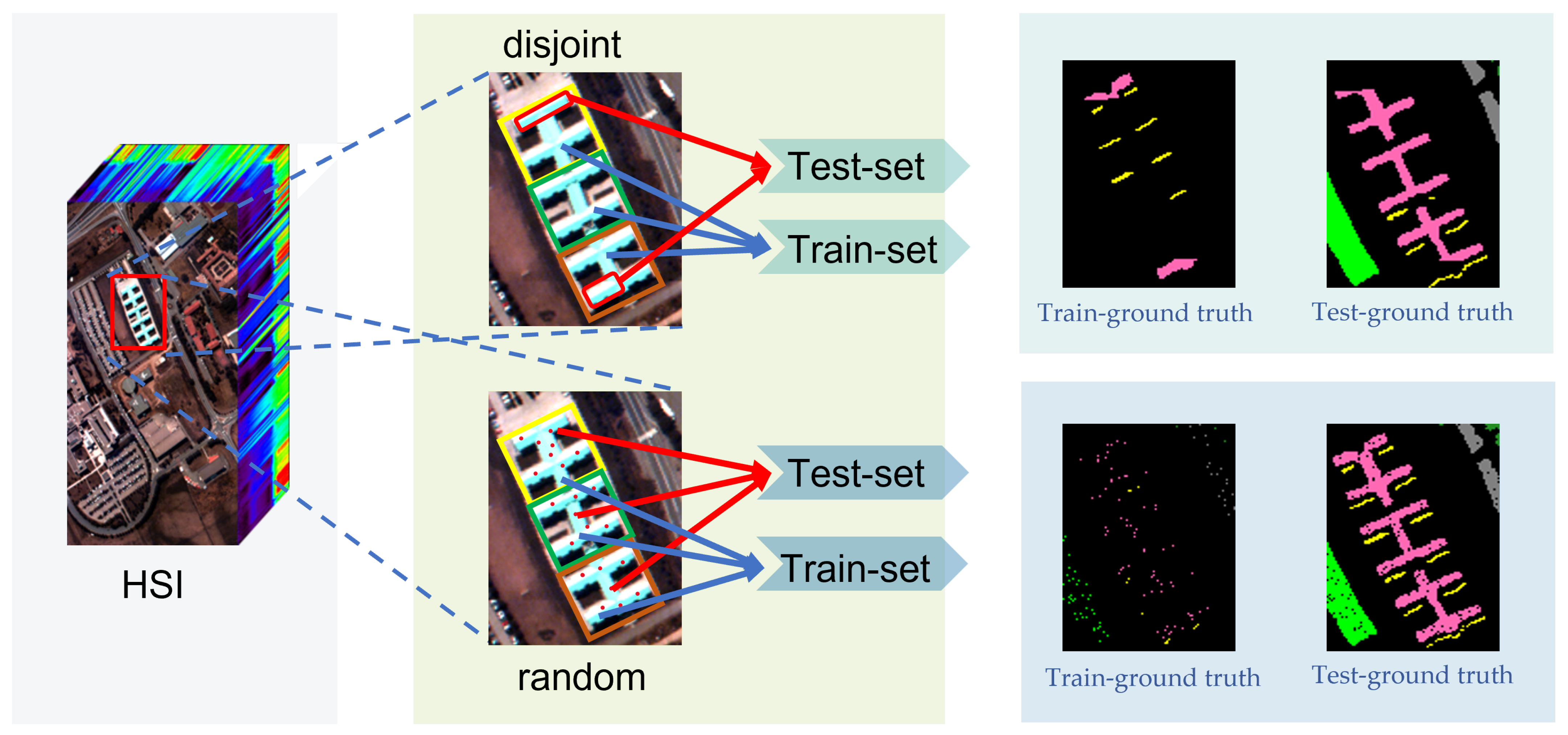
Exploring the impact of information leakage on the generalization ability of HSI classification models should be validated with multiple homogeneous datasets. Specifically, the classification ability of this model is first obtained by training it on a single dataset. Other homogeneous datasets are then used as test samples for classification without retraining. Finally, the classification accuracy of the latter is compared with that of the former. The difference values can intuitively reflect the effect of information leakage on generalization ability. However, due to the lack of corresponding homogeneous datasets, this process can only be approximated by spatially disjoint sampling strategies. Spatially disjoint sampling means that the training set pixels are adjacent to each other during HSI sampling to minimize the overlap between training and test samples. As shown in Figure 4, this sampling method not only reduces the information of the test set directly involved in training the network effectively, but also makes more test set samples far from the training set samples in terms of spatial location. Moreover, from the perspective of spectral variation, such sampling methods are more likely to learn only some spectral generalization features and partial variation features due to mixed endmembers. Therefore, the training set and the test set, which are spatially disjoint partitioned, can be approximated as two homogeneous datasets with strong independence.

This approximation process can intuitively reflect the qualitative effect of information leakage on the generalization ability of the model to a certain extent, but it cannot be used as an accurate quantitative indicator to assess the generalization ability of the model. There are three reasons for this:

1.

It is an approximate process, not exactly equivalent to constructing a homogeneous dataset, because spatially disjoint sampling is not completely immune to information leakage. In the spatially disjoint sampling strategy, the samples at the edges of the training set still contain some test pixels. These patches lose some spatial information to some extent;

2.

It was experimentally found that the difference of classification accuracy between spatially disjoint sampling strategies and random sampling strategies was related to the chosen datasets;

3.

Some semi-supervised methods can make the model learn the test data in a spatially disjoint sampling way by constructing pseudo-labels for unlabeled samples [53]. As a result, the networks can achieve great classification accuracy under both sampling methods. However, the learning paradigm still suffers from information leakage and needs to be retrained when classifying other homogeneous datasets.

2.3. Methods to Mitigate the Impact of Information Leakage

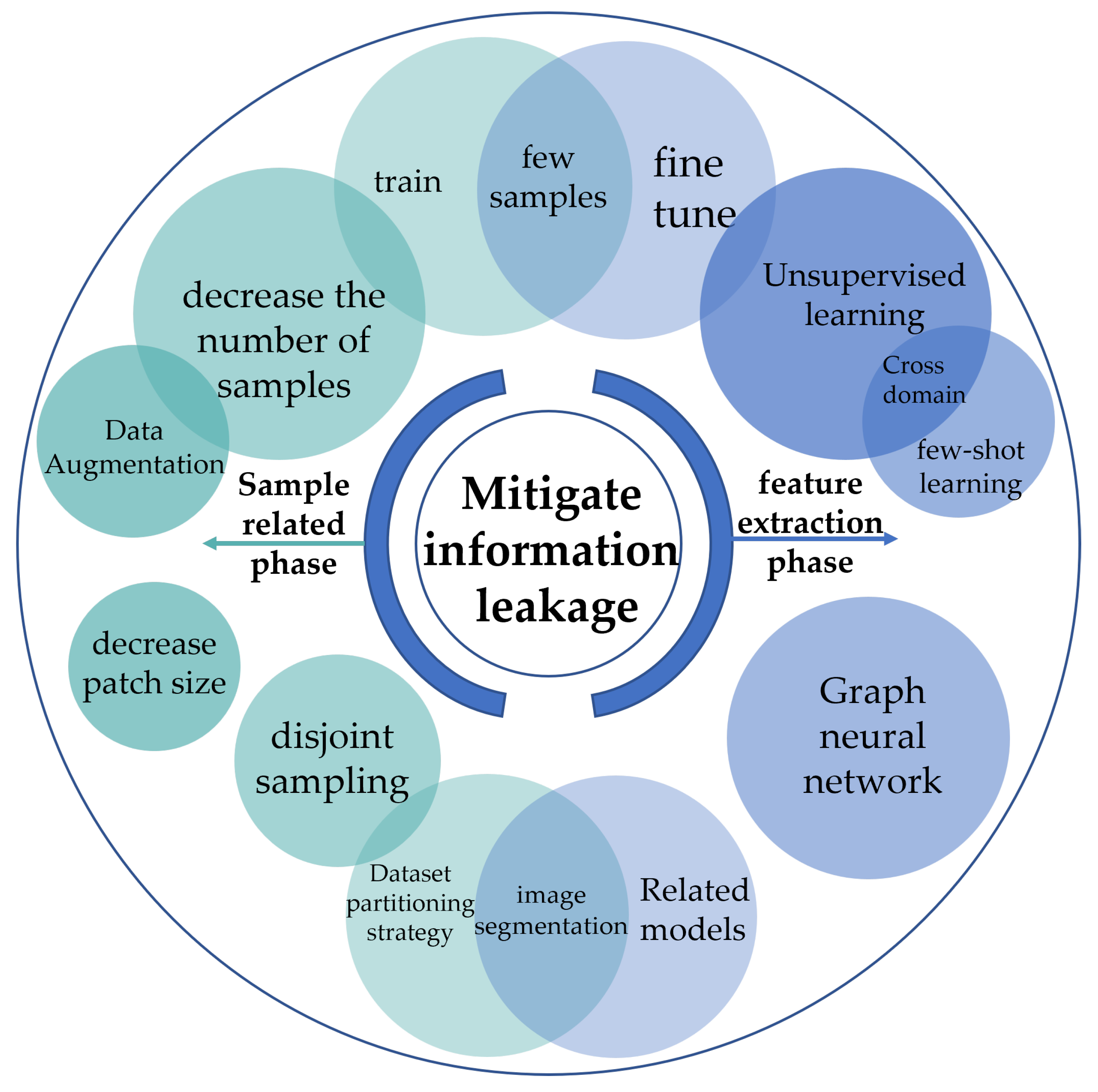
Some studies [36,48] visualize the impact of information leakage by comparing random sampling strategies with spatially disjoint sampling strategies and highlight the issue of generalization ability in current partial models. As shown in Figure 5, two aspects are considered to mitigate information leakage. The first is to consider the sample-related phase, that is, to reduce the leakage of information from the source by reducing the number of samples, assuming that the classification model has been determined. Moreover, spatially disjoint sampling strategies can be used so that the test samples do not overlap with the training samples as much as possible. Second, considering from the feature extraction phase, under the condition of a given number of labeled samples, the impact of information leakage is further mitigated by using feature extraction methods such as unsupervised and FSL. The former aims at alleviating information leakage from data sources, while the latter can enhance the generalization ability of models between homogeneous datasets.

2.4. Sample-Related Phase

Reducing the number of samples directly reduces the test set information involved in training. If the patch input format is used in the deep learning model, then the test pixels in this patch are also fed into the network. As shown in Figure 6, in a given certain HSI dataset, there are a total of N labeled pixels, the patch size is $h\times w$, and n samples are taken for training. Let $g_i$ denote the number of unknown background pixels in the patch of the $i^{\prime }$th test sample. For the random sampling strategy, each labeled pixel is split independently into a training set with probability $p=n/N$ and a test set with probability $q=1-p$. Let $l_i$, $m_i$ denote the $l^{\prime }$th row and $m^{\prime }$th column in the patch corresponding to the $i^{\prime }$th test sample. If the $i^{\prime }$th test sample is not trained into the network, then all patches containing this pixel are not in the training set. Thus, when the event $A_i$ represents that the information of the $i^{\prime }$th test sample is not directly involved in training the network, the probability of $A_i$ is expressed as follows:

$$P\left(A_i\right)=\prod _{l=1,m=1}^{l\ne \frac{h}{2},m\ne \frac{l}{2}}{q}_{i_{(l,m)}}={(1-\frac{n}{N})}^{w\times h-1-g_i},1\le l\le h,1\le m\le w$$

(1)

Moreover, the expectation of the number of test set samples X, which are not directly involved in the training of the network, is expressed as follows:

$$E\left(X\right)=\sum _{i=1}^{N-n}P\left(A_i\right)\times 1=\sum _{i=1}^{N-n}{(1-\frac{n}{N})}^{w\times h-1-g_i},1\le l\le h,1\le m\le w$$

(2)

From the above equation, increasing $E\left(X\right)$ can be achieved by reducing the size of the input patch and the number of training sample, thus reducing the information leakage. Experiments in [31] show that even if the sample neighborhood size is set to $3\times 3$, when more than 10% of the samples are used for training, the number of unleaked test pixels will drop below 50%. In the case of the patch size being $9\times 9$, nearly all test pixels are exposed to the network training stage.

2.4.1. Data Augmentation Strategies

While training a network with a limited number of samples reduces information leakage to some extent, it also significantly decreases accuracy. Therefore, several preprocessing strategies such as data augmentation have been introduced into the field of HSI image classification. Common data augmentation methods include flipping, radiation noise, and mixture noise. Flipping means that each training sample is flipped independently in horizontal and vertical directions with a certain probability.

The radiation noise can be described by the formula:

$$x_i^{\prime }={\alpha }_{rn}{x}_i+{\beta }_{rn}{n}_{noise}$$

(3)

where $x_i$ and $x_i^{\prime }$ represent the $i^{\prime }$th original training sample and the new sample, respectively. ${\alpha }_{rn}$ represents a controlled random coefficient of the degree to which the information of the original sample is preserved, and its range is commonly controlled from 0.9 to 1.1. $n_{noise}$ is the noise signal that follows the standard normal distribution, and ${\beta }_{rn}$ is a constant to control the noise intensity.

The mixture noise is the sum of two samples of the same class according to a certain weight, followed by the addition of a noise signal. This process can be formulated as follows:

$$x_i^{\prime }=\frac{{\alpha }_{mn1}{x}_i+{\alpha }_{mn2}{x}_j}{a_{mn1}+a_{mn2}}+{\beta }_{mn}{n}_{noise}$$

(4)

where $a_{mn1}$ and $a_{mn2}$ are the weights of the two original samples in the new sample, and ${\beta }_{mn}$ represents the coefficient that controls the noise intensity.

Zhang et al. [43] considered the cloud occlusion in the original image data. The data augmentation strategy of block random erasure is added to simulate cloud occlusion conditions. In order to alleviate the overfitting problem caused by limited samples, Zhang et al. [54] used three angles of rotation and two directions of flipping in the proposed dual-channel convolutional network. The data augmentation method increased the training samples by six times. Zhang et al. [55] performed data augmentation in two steps. First, the original image block samples are flipped and then Gaussian noise is added to generate additional training samples. Li et al. [56] compared the commonly used data augmentation methods and proposed a novel method using pixel-block pairs (PBP) of deep CNN to increase the number of samples. This data augmentation method needs to correspond to its proposed PBP-CNN model. Specifically, pixel-blocks for training are first constructed and then each pixel-block is paired with all other pixel-blocks to form new samples. If the labels of the two pixel-blocks are consistent, the new sample is given the same label. If the labels of two pixel-blocks do not coincide, the label will be zero. This data augmentation method significantly increases the number of training samples for its proposed model. Chen et al. [57] noticed the difference between the test samples and the new training samples through the data augmentation, which hinders the classification performance. A similarity score obtained by Siamese network is proposed to reduce this difference. Some studies have considered the class imbalance problem in HSIs and performed different degrees of data augmentation for different classes [58,59].

With the rise of Generative Adversarial Networks (GANs) [60], related data augmentation methods have also been introduced into HSI classification tasks. GANs consists of a generator and a discriminator. The former is used to capture the data distribution and generate samples. The later estimates the probability of sample authenticity, and the generator and discriminator compete with each other to train the network. The HSI samples generated by the generator learn the spatial context information in the original HSI. The discriminator controls the difference between the generated samples and the real samples. Therefore advanced, these additional samples can be used as training samples to participate in the training of the classification model. Neagoe et al. [61] designed a Generative Adversarial Network (GAN) under a deep CNN framework in order to generate additional training samples. The accuracy is significantly improved compared to the deep CNN model without GAN, which demonstrates the effectiveness of GAN for data augmentation. Dam et al. [62] considered the problem of class imbalance resulting in the inability to generate samples of partial classes, and proposed a three-player spectral GAN to generate effective samples even for classes with a few samples. However, GAN-based data augmentation also faces some challenges, such as the mode collapse and inefficient description of HSIs spectral spatial features. Mode collapse means that the generator produces only a part of the modes in the data distribution and fails to cover all the modes. On this basis, Liang et al. [63] proposed a semi-supervised deep learning model based on GAN and attention mechanism, which alleviated the above two problems by using mean minimization loss and constructing a spectral–spatial attention module. Wang et al. [64] noticed that most existing GAN-based classification methods pre-assume that HSI data are mapped according to basic distributions such as Gaussian distribution when generating samples. However, due to the complexity of HSI data, the underlying structure of the samples generated by GAN has not been sufficiently characterized. Therefore, a novel model named Graph Adversarial Learning is proposed to combine GAN and graph learning to explore the internal structure of HSI data more comprehensively.

2.4.2. Spatially Disjoint Sampling Strategies

In addition to reducing the number of training samples, the impact of information leakage can also be mitigated by using some spatially disjoint sampling strategies. These strategies increase the Euclidean distance between training samples and testing samples, and effectively reduce the spatial dependence between them. In the following, some of the existing spatial disjoint sampling strategies are enumerated:

• Controlled Random Sampling Strategy: Liang et al. [45], inspired by the region-growing algorithm, performed controlled random sampling through the following three steps. First, disconnected partitions are selected for each class. Second, training samples are generated in each partition by expanding the region with seed pixels. Finally, after all classes have been processed, the samples in the labeled growing region are used as the training set and the remaining samples are used as the test set. At the same time, a paradox of sampling methods is presented in this work. Not only should the overlap between the test set and the training set be avoided as much as possible, but also the training samples should contain sufficiently different classes of spectral data variants. The former tends to select training samples centrally, while the latter requires training samples to be distributed in more different regions;
• Continuous Sampling Strategy: In order to reduce the influence of random sampling on classification accuracy, Zhou et al. [34] adopted the sampling method of sampling continuously from local regions for each class. This method selects different local regions, which do not completely avoid data leakage. However, the training samples contain more spectral variations;
• Cluster Sampling Strategy: Hansch et al. [65] proposed a cluster sampling method to minimize the correlation between the training set and the test set. For each class, it is clustered into two clusters according to its spatial coordinates. The training samples are randomly selected from a cluster, and the remaining classes are used as the test set;
• Density-Based Clustering Algorithm Sampling Strategy: Lange et al. [66] detect subgroups in a set by recursively evaluating the density threshold of neighbor points around the sample with parameter $ϵ$ as the search radius. Therefore, independent regions can be determined by clustering the coordinates of pixels of a particular class.

In addition, several scholars have combined the HSI classification problem with the segmentation problem and proposed different strategies for partitioning datasets. These partitioning strategies are based on segmentation models, which effectively alleviate the information leakage problem. Nalepa et al. [32] proposed a datasets partition method based on random patches, which effectively avoided the test set information participating in the training of the network, and realized the segmentation task of HSI through 1D convolution. However, some classes with no training samples may exist. Zou et al. [49] split the HSI dataset into regions of the same size. Regions containing only pixels of the same type form part of the test set, and the remaining regions containing pixels of multiple types are divided into training set, validation set and test set for cross validation. In this work, the authors propose a spectral spatial 3D fully convolutional network classifier to classify all pixels in each patch sample. The model performs the segmentation task under the assumption that the overlap between test and training samples is avoided. Li et al. [67] combined PCA, attention mechanism and U-net [68] to propose a deep learning model suitable for HSI image segmentation tasks. When constructing samples, a non-overlapping sliding window strategy combined with a judgment mechanism is introduced to split the HSI into training, test, and validation sets. The proposed method effectively avoids information leakage and the absence of partial classes in the training set.

These spatially disjoint sampling strategies result in more objective model classification results. Therefore, the difference between the classification accuracy obtained by random sampling and spatially disjoint sampling above is frequently used to evaluate the influence of the model on information leakage [48,53]. However, in Figure 7, the amount of information leakage, the classification accuracy of the model under different sampling strategies, and the generalization ability of the models between homogeneous datasets should be evaluated in different ways. The difference in classification accuracy between random sampling strategies and disjoint sampling strategies is affected by numerous aspects such as datasets, and various hyperparameters. This also suggests from another perspective that the difference in classification accuracy between these sampling methods cannot be directly used as an accurate criterion for the generalization ability. However, the comparison reflects the impact of information leakage to some extent.

2.5. Feature Extraction Phase

This section introduces several learning paradigms and networks that mitigate the information leakage problem from a feature extraction perspective, including unsupervised learning, few-shot learning (FSL), and graph neural networks (GCNs).

2.5.1. Unsupervised Learning and Semi-Supervised Learning

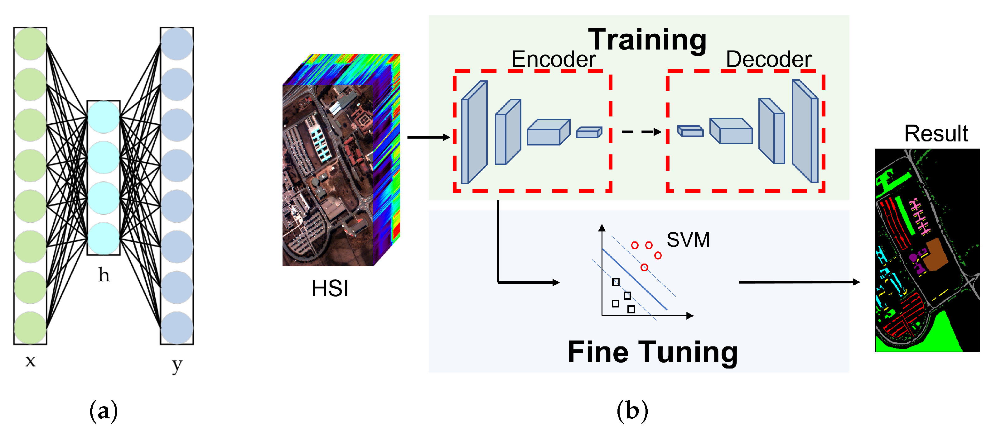
Beyond data augmentation and dimensionality reduction, unsupervised learning and semi-supervised learning are suitable for classification tasks with a limited number of samples. SAE is one of the commonly used unsupervised feature extraction models, which consists of multiple AE modules. Figure 8a is the basic structure of the AE. Where x is the input feature, h is the hidden layer feature, and y is the output feature. The training process is represented by the following formulas:

$$h=f\left(w_{h}x+b_h\right)$$

(5)

$$y=f\left(w_{y}x+b_y\right)$$

(6)

where $w_h$ and $b_h$ are the weights and biases from the input layer to the hidden layer and $w_y$ and $b_y$ are the weights and biases from the hidden layer to the output layer. $f\left(·\right)$ is the activation function. The loss function is then constructed using the Euclidean distance between x and y (minimize ${\left|\right|x-y\left|\right|}^2$). During training process, x is approximated by mapping h to y. Therefore, h can be used as a feature for x.

Unsupervised learning is suitable not only for tasks with limited labeled samples, but also does not require the use of labels in the feature extraction phase. From this perspective, unsupervised learning has the potential to alleviate information leakage. Generally, in HSI classification models, unsupervised learning is used for feature extraction, followed by fine-tuning with a classifier such as SVM or softmax in a supervised way to perform the final classification [38,39]. Inspired by contrastive learning and transformer model [69], Hu et al. [70] introduced an advanced contrastive learning framework in the HSI classification field, namely bootstrap your own latent (BYOL). A two-layer transformer mode is used as the feature extractor without using any convolutional or recurrent units. After unsupervised training, the SVM classifier and a limited number of labeled samples are used for the final classification. On this basis, Li et al. [71] proposed a BYOL model based on random occlusion and studied the influence of different occlusion strategies. Liu et al. [72] proposed an adversarial adaptation network in the HSI unsupervised classification task. The model generates domain-invariant features through adversarial learning. Domain-invariant features are those that remain consistent or similar across different domains. Sun et al. [52] proposed an unsupervised spectral motion feature learning framework based on optical flow estimation, which is commonly used to obtain motion information of dynamic objects. The proposed framework treats spectral changes as motion changes during feature extraction. After pre-training on sufficient unlabeled samples, the model has the ability to directly test on different datasets. Gao et al. [73] considered that existing HSI classification methods based on meta learning would require a large number of labeled samples to construct source domain datasets. Therefore, an unsupervised meta-learning method with multiview constraints is proposed. The multiview features consist of different bands of the same sample.

Semi-supervised learning also requires a limited number of samples. However, semi-supervised methods generally use these samples to assign pseudo-labels to some test samples to obtain additional samples used for training. Fang et al. [74] used multiscale spatial information to train a CNN-based classifier through self-learning, and retained pseudo-label samples with high confidence during prediction for the next iteration training. Zhao et al. [75] noticed the problem that random sampling threatens the independence of samples, and proposed a deep mutual-teaching model. The model uses controlled random sampling method to select training samples. Specifically, the edge and texture information of the original HSI is extracted by extended morphological profiles and edge-preserving filter, and then trained by two CNN models with the same structure but different parameters. After training, partial test samples are predicted separately, and each CNN model assigns samples with high confidence pseudo-labels and merges them with the training set of another CNN model before retraining, repeating the above procedure several times. During training of the model, the training samples are obtained through spatially disjoint partitioning. However, the pseudo-labeled samples are not sampled by the disjoint strategy. The spatial correlation between the pseudo-labeled samples and the test samples is not reduced. This is one of the important reasons why semi-supervised learning based HSI classification methods still achieve high accuracy under spatially disjoint sampling patterns. However, the models are contrary to the original intention of using spatially disjoint sampling strategies. The spatial autocorrelation between the samples participating in the network training and the test samples is non-negligible. The pseudo-labeled samples are all from the same dataset. Training the network with these samples essentially trains the network’s ability to fit this dataset, resulting in overly optimistic classification accuracy. On the other hand, considering practical applications, this approach still needs to be retrained when testing on different homogeneous datasets. Since a single training stage needs to be repeated, the computational cost is relatively high. In addition, this situation also reflects the difference in classification accuracy obtained by different sampling methods, which cannot be used as a general criterion to evaluate the extent of information leakage impact or generalization ability of the model.

Moreover, related deep learning methods using graphs are introduced into the field of HSI classification. Graph structure is a general non-Euclidean structure. In HSI classification tasks, pixels are often considered as nodes of a graph, and the adjacency matrix A is formed as a function of the distance between different nodes. Usually, the information of this graph is added to the adjacency matrix. The final form described by the following formula:

$$\tilde{A}=A+I$$

(7)

where I is the identity matrix, and then normalized by the degree matrix D. Forward propagation is carried out as follows:

$$H^{\left(l+1\right)}=h\left({\tilde{D}}^{-\frac{1}{2}}\tilde{A}{\tilde{D}}^{-\frac{1}{2}}{H}^{\left(l\right)}{W}^{\left(l\right)}+b^{\left(l\right)}\right)$$

(8)

where $h\left(·\right)$ is the activation function, b are the biases, W are the learnable weights, and l is the current number of layers.

Since the graph consists of training samples in some models, the involvement of test set information in the training stage is strictly avoided. Hong et al. [76] randomly divided the dataset into subregions, and the training samples of each subregion formed a graph for the input network. The minibatch algorithm is introduced to implement graph convolutional neural networks in supervised learning. The proposed model combined with a 3D CNN achieves good performance and avoids information leakage to some extent. In the field of HSI classification, graph-structured algorithms are more commonly used for semi-supervised classification. Sha et al. [77] proposed a semi-supervised classification model based on graph attention network, which used spectral spatially distance information to encode features. Furthermore, the model introduces the spectral spatial similarity of neighboring pixels as different attention weights into the convolution operation at each node, which is finally classified by the graph convolutional network. However, using unlabeled samples may degrade classification performance. He et al. [78] proposed a semi-supervised model based on constraint graph. In this work the raw HSI data is preprocessed by image fusion and recursive filtering feature algorithm, and then the graph-to-sample correlation is enhanced by computing the affinity matrix. The affinity matrix is an essential statistical technique for measuring the mutual similarity between a set of data points. Finally, a particle competition and cooperation mechanism is introduced to dynamically label and correct pseudo-labeled samples. Xi et al. [79] proposed a semi-supervised graph prototypical network. This model constructs an adjacency matrix using the entire dataset as a graph, and extracts spectral spatial features through a graph convolution network. On this basis, a prototypical layer was added to the model, and a Cross-Entropy loss function containing distance information was designed. Cai et al. [80] proposed a hypergraph structured autoencoder, in which each pixel of the HSI serves as a vertex of the hypergraph, and uses the closest K neighbors of the vertex to construct hyperedges. This work incorporates the hypergraph into the autoencoder model to train the network through unsupervised or semi-supervised learning paradigms.

2.5.2. Few-Shot Learning

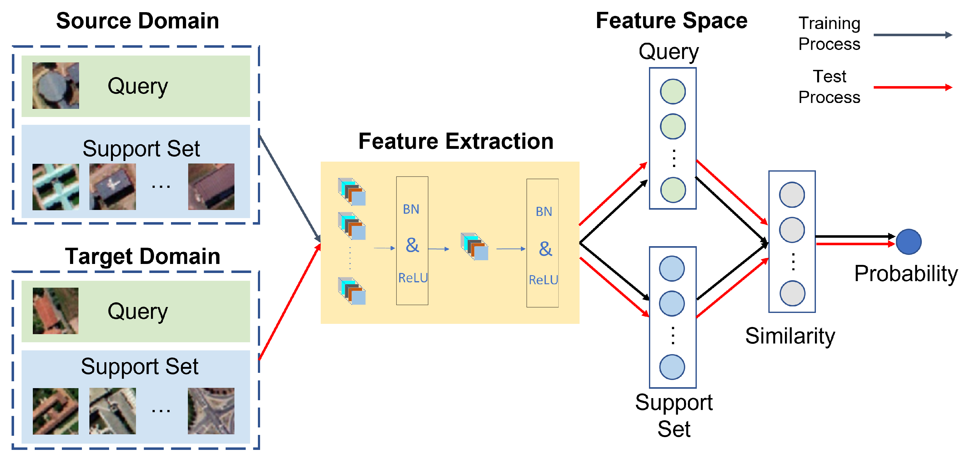
FSL is a type of meta-learning, which is an emerging deep learning model in recent years to address the problem of limited labeled samples. Different from other HSI classification models based on deep learning, FSL aims to make the model learn the similarity between samples of the same class, rather than make the model “recognize” the target samples. As shown in Figure 9, The procedure is generally divided into three steps. First, in each forward propagation, the features of a pair of samples are extracted and mapped to the feature space. Second, the distance or similarity between different samples in the feature space is judged by a specific transformation. Finally, the test sample is compared with the support set to determine if it belongs to the same class. This approach does not use target domain samples during training, or by using a limited number of samples to adapt the model to different domains. Therefore, the FSL model effectively mitigates information leakage and improves the independence between training and test sets. Similar to transfer learning models, FSL models can be tested on different datasets in the target domain after being trained in the source domain at low computational cost. At the same time, because the features extracted are used to judge the similarity between samples rather than identify samples, the FSL models achieve superior classification performance in the case of limited samples (support set), which is relatively suitable for HSI classification tasks.

Considering that small support sets easily lead to model overfitting, Pal et al. [28] combined dropout and dropblock in FSL, and minimized the Bayesian approximation of model uncertainty through Monte Carlo approximation. Monte Carlo approximation is a method used to estimate complex mathematical quantities using random sampling. The work improves the objective function and adds the true class prediction variance to further enhance the generalization confidence of the model. Bai et al. [29] proposed an FSL model combining a 3D local channel attention mechanism and residual learning. In contrast to traditional similarity classification using the mean of the embedded features, this model uses a classifier that adaptively increases the margin between different class subspaces and shows superior performance. Tang et al. [81] used multiscale input to obtain semantic information of different scales, and proposed a spatial–spectral prototypical representation suitable for multiscale HSIs based on the feature extraction algorithm theory of ladder structure. Sun et al. [82] proposed a novel FSL classification method, which introduced the Earth mover’s distance (EMD) as a measure to judge the similarity of embedded features. EMD is designed to measure the distance between the weighted distributions of two domains and is used to generate similarity scores between samples from the query set and the support set. In order to further reduce the domain shift caused by cross-domain and strengthen the adaptability of the model to the data distribution of the target domain, Li et al. [83] proposed a novel deep cross-domain few-shot learning (DCFSL) method. In this model, samples from the source and target domains are trained simultaneously. The network can learn transferable knowledge in the source classes and discriminative embedding model for the target classes. Gao et al. [84] were inspired by the relational network and combined it with FSL. The proposed model further utilizes spectral spatial information to learn the similarity between different samples. Moreover, the model uses multiple datasets to form the source domain, which improves the generalization ability of the model.

3. Results

3.1. Datasets

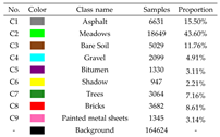
The University of Pavia (UP) dataset was captured in 2001 by RPSIS sensors including the University of Pavia in Italy and its surrounding urban areas. Its pixels are divided into nine classes and backgrounds. The dataset consists of $610\times 340$ pixels with a spatial resolution of 1.3 m. Its spectrum ranges from 0.43 to 0.86 µm and is divided into 115 spectral bands. Considering the noise pollution, 13 bands are removed, then the final size is $610\times 340\times 103$. However, only 42,776 pixels were labeled with the class and the remaining pixels were identified as backgrounds.

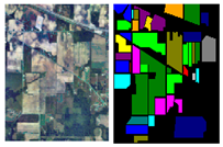
The Indian Pines (IP) dataset was collected by AVIRIS sensor at the Indian Pine Test Site in northwest Indiana in 1992. The dataset consists of 16 crops and backgrounds. The distribution of the target ground-based objects mostly presents a regular shape, covering $145\times 145$ pixels areas, with a spatial resolution of 20 m. The spectrum ranges from 0.4 to 2.5 µm and is divided into 244 spectral segments. Moreover, the effect of noise is considered and some bands are removed. The size of the final corrected dataset is $145\times 145\times 200$, in which about half of these pixels are used to label objects, and the remaining pixels are used to mark the background.

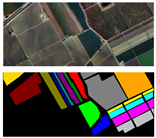
The Salinas Valley (SV) dataset is collected over several farmland in Salinas Valley, California. It is composed of $512\times 217$ pixels. As with the IP dataset, both were collected by the AVIR sensor and some water absorption bands were removed to account for noise effects. The size of the corrected dataset is $512\times 217\times 204$. Among them, 54,129 pixels can be used for classification, which are divided into 16 classes, and the remaining 56,975 pixels are regarded as the backgrounds. Unlike the IP dataset, the SV dataset has a better spatial resolution of up to 3.7 m.

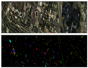
The GRSS-DFC-2013-Houston (HS) dataset was collected by the National Center for Airborne Laser Mapping at the University of Houston in June 2012, and was distributed for the 2013 IEEE Geoscience and Remote Sensing Society (GRSS) Image Analysis and Data Fusion (IADF) Contest [85,86]. The HSI consists of 144 spectral bands in the 0.38 µm to 1.05 µm region. In terms of spatial scale, the size of the dataset is $349\times 1905$ with a spatial resolution of 2.5 m, and consists of 15 categories and backgrounds.

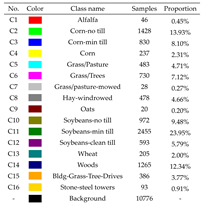
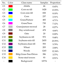
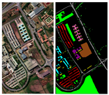
The false color map, ground truth (GT) map, number and proportion of various samples of each dataset are shown in

Table 2. Indian Pines dataset, Salinas Valley dataset, University of Pavia dataset.

Indian Pines	Salinas Valley	Houston
University of Pavia

. The proportion reflects the imbalance between the classes in each dataset. The problem causes the deep learning model to shift more attention to the classes with more samples. Therefore, the accuracy of the classes with less samples decreases. To tackle this problem, some works [57,62] considered the imbalance between classes and alleviated the problem through data augmentation.

3.2. Experimental Setups

All experiments in this paper describe the effect of information leakage through two different sampling strategies, one with random sampling and the other with continuous sampling (spatially disjoint sampling). As shown in

Table 3. Experimental setup.

Experiments	Models		Datasets	The Number of Samples
Convolutions in different dimensions	LR-1D-CNN RSSAN SS-3D-CNN	D-1D-CNN R-2D-CNN D-3D-CNN	UP SA HS	0.3%, 0.5%, 0.75%, 1%, 3% 5%, 7%, 10%, 15%, 20%
Data augmentation with disjoint sampling	LR-1D-CNN SS-3D-CNN	R-2D-CNN	UP HS	3, 5, 7, 9, 11, 13 (per class)
Cross-domain learning with disjoint sampling	DCFSL SMF-UL	RN-FSC UM2L	IP UP	3, 5, 7, 9, 11, 13 (per class)

, in order to explore the effectiveness of different information leakage mitigation methods more comprehensively, the following three experiments are designed in this paper. As shown in

Table 4. Some hyperparameters related to these models.

Models	Learning Rate	Epoch	Patch Size	Batch Size	Optimizer
LR-1D-CNN	0.01	300	1	100	SGD
D-1D-CNN	0.01	100	1	100	SGD
RSSAN	0.001	100	9	128	SGD
R-2D-CNN	0.001	100	9	128	SGD
SS-3D-CNN	0.001	100	5	100	SGD
D-3D-CNN	0.001	100	5	100	SGD
SMF-UL	0.0001	1000	-	4	Adam
Models	Learning rate	Episode	Patch size	Way	Optimizer
DCFSL	0.001	20,000	9	9	Adam
RN-FSC	0.001	10,000	9	9	Adam
UM2L	0.001	40,000	9	9	Adam

, except for the number and sampling method of training samples, the remaining hyperparameters related to the model (such as learning rate, epoch, patch size) refer to the settings in the relevant works as much as possible. Each training was repeated independently five times and the corresponding test results were averaged to reduce errors. Experiment 1 and Experiments 2 use the overall accuracy (OA) under different sampling strategies to evaluate the degree of information leakage. OA, average accuracy (AA), and kappa coefficient are used to evaluate the model performance in experiment 3.

3.2.1. Experiment 1: Convolutions in Different Dimensions

This experiment aims to compare the classification accuracy of the supervised learning 1D-CNN, 2D-CNN, and 3D-CNN models. Different sampling methods, number of training samples and datasets were used to reflect the impact on information leakage. For this experiment, UP, IP, and HS datasets were used and six models were selected. The 1D-CNN model uses a one-dimensional CNN with L2 regularization and logistic regression (LR-1D-CNN) proposed by Chen et al. [87] and a deep convolutional neural network (D-1D-CNN) used by Hu et al. [88]. The 2D-CNN model selected is the residual spectral-spatial attention network proposed by Zhu et al. [89] (RSSAN) and recurrent 2D convolutional CNN (R-2D-CNN) proposed by Yang et al. [90]. The 3D-CNN model selected is a spectral-spatial 3D-CNN (SS-3D-CNN) used by Li et al. [26] and a deep 3D convolutional neural network (D-3D-CNN) proposed by Hamida et al. [91]. The number of training samples in this experiment is divided into two levels. Furthermore, we specify that less than 3% of the samples are limited samples, and design five different numbers of samples at small intervals, namely 0.3%, 0.5%, 0.75%, 1%, and 3%. In the experiment, we specify that more than 3% of the samples are sufficient samples, so the intervals are increased, namely 5%, 7%, 10%, 15%, 20%.

3.2.2. Experiment 2: Data Augmentation with Disjoint Sampling

This experiment explores the impact of few training samples and data augmentation on information leakage. Specifically, LR-1D-CNN, R-2D-CNN, and SS-3D-CNN used in Experiment 1 are selected as models. we choose UP and HS datasets and select 3, 5, 7, 9, 11, 13 samples for each class. In addition, radiation noise and mixed noise data augmentation are used separately on the 1D-CNN model. The data augmentation methods of flipping and random radiations are used on 2D-CNN and 3D-CNN models. Finally, the differences in classification accuracy between the two sampling methods are compared to explore the effectiveness of few training samples and data augmentation in mitigating information leakage.

3.2.3. Experiment 3: Cross-Domain Learning with Disjoint Sampling

The experiment integrates both factors of the sample-related phase and the feature extraction phase. In this experiment, some FSL models and unsupervised learning-based models are used with few samples. For the FSL models, we select DCFSL proposed by Li et al. [83] and a few-shot classification model based on relation network (RN-FSC) proposed by Gao et al. [84]. For the unsupervised learning-based models, we chose the unsupervised spectrum motion feature learning framework (SMF-UL) proposed by Sun et al. [52] and an unsupervised meta-learning method with multiview constraints (UM2L) proposed by Gao et al. [73]. In this experiment, the IP dataset is used as the source domain dataset and the UP dataset is used as the target domain dataset, and 3, 5, 7, 9, 11, 13 samples are selected for each target class. Finally, the classification accuracy of different sampling methods is used to compare the effectiveness of such models in mitigating the impact of information leakage.

3.3. Experimental Results and Discussion

3.3.1. Analysis of Convolutions in Different Dimensions

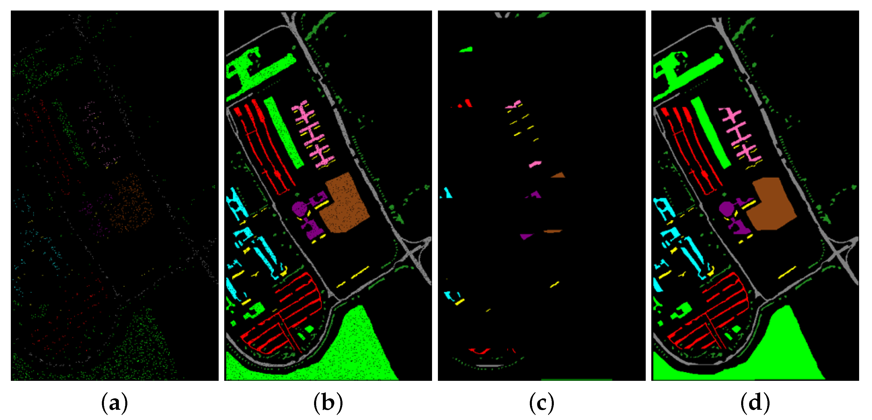
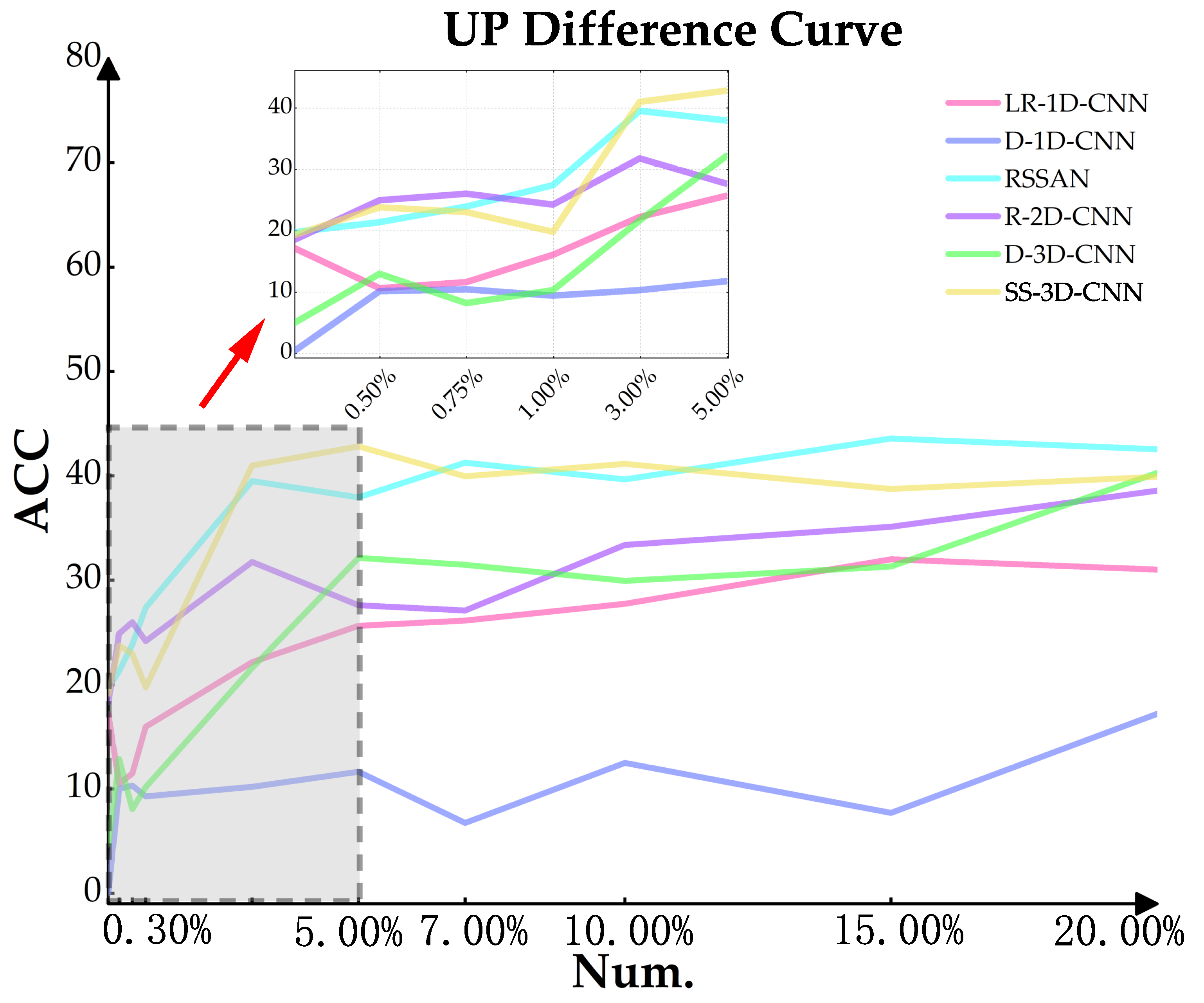
The experimental results are listed in

Table 5. OA and difference of different CNN models using random sampling strategy and spatially disjoint sampling strategy on the UP dataset.

	LR-1D-CNN			D-1D-CNN			RSSAN
Num.	Random	Disjointed	Diff	Random	Disjointed	Diff	Random	Disjointed	Diff
0.30%	72.018	54.831	17.187	53.672	53.608	0.064	66.950	47.302	19.648
0.50%	72.610	62.114	10.496	64.269	54.242	10.027	71.589	50.286	21.303
0.75%	73.324	61.825	11.499	66.435	56.101	10.334	72.011	48.159	23.852
1%	74.352	58.380	15.972	67.381	58.088	9.293	75.802	48.434	27.368
3%	76.298	54.142	22.156	71.557	61.360	10.197	82.451	42.944	39.507
5%	77.264	51.633	25.631	72.993	61.330	11.663	83.544	45.613	37.931
7%	82.012	55.878	26.134	74.409	67.668	6.741	89.169	47.909	41.260
10%	82.886	55.138	27.748	75.955	63.458	12.497	89.946	50.287	39.659
15%	87.850	55.837	32.013	72.770	65.050	7.720	91.976	48.388	43.588
20%	87.110	56.090	31.020	75.824	58.627	17.197	93.691	51.139	42.552
	R-2D-CNN			D-3D-CNN			SS-3D-CNN
Num.	Random	Disjointed	Diff	Random	Disjointed	Diff	Random	Disjointed	Diff
0.30%	71.774	53.473	18.301	58.490	53.810	4.680	74.434	55.303	19.131
0.50%	75.693	50.800	24.893	66.759	53.901	12.858	80.119	56.382	23.737
0.75%	76.997	51.031	25.966	70.197	62.126	8.071	84.368	61.407	22.961
1%	77.710	53.535	24.175	73.937	63.759	10.178	85.460	65.725	19.735
3%	81.160	49.416	31.744	77.996	56.386	21.610	91.599	50.610	40.989
5%	84.227	56.621	27.606	86.267	54.129	32.138	94.692	51.865	42.827
7%	87.673	60.574	27.099	89.138	57.670	31.468	95.297	55.338	39.959
10%	92.244	58.857	33.387	88.253	58.314	29.939	96.016	54.868	41.148
15%	93.097	57.964	35.133	89.989	58.661	31.328	96.267	57.514	38.753
20%	93.715	55.133	38.582	95.417	55.148	40.269	96.690	56.781	39.909

and

Table A1. OA and difference of different CNN models using random sampling strategy and spatially disjoint sampling strategy on the SV dataset.

	LR-1D-CNN			D-1D-CNN			RSSAN
Num.	Random	Disjointed	Diff	Random	Disjointed	Diff	Random	Disjointed	Diff
0.30%	59.045	59.594	−0.549	20.822	21.470	−0.648	60.837	42.276	18.561
0.50%	60.202	59.999	0.203	20.823	20.841	−0.018	69.590	45.765	23.825
0.75%	63.131	64.457	−1.326	20.823	20.838	−0.015	74.593	49.205	25.388
1%	64.885	65.827	−0.942	20.822	20.860	−0.038	76.990	49.475	27.515
3%	78.754	73.525	5.229	29.864	29.869	−0.005	72.759	64.716	8.043
5%	79.448	74.366	5.082	50.213	48.883	1.330	81.496	59.244	22.252
7%	82.872	75.944	6.928	59.895	58.688	1.207	85.848	75.773	10.075
10%	82.525	71.369	11.156	63.810	64.739	−0.929	89.772	77.211	12.561
15%	83.273	76.599	6.674	71.429	68.269	3.160	90.383	80.578	9.805
20%	85.915	76.794	9.121	76.399	70.411	5.988	91.262	80.698	10.564
	R-2D-CNN			D-3D-CNN			SS-3D-CNN
Num.	Random	Disjointed	Diff	Random	Disjointed	Diff	Random	Disjointed	Diff
0.30%	60.746	46.042	14.704	40.217	38.741	1.476	78.021	55.864	22.157
0.50%	66.633	48.268	18.365	49.674	40.294	9.380	76.395	49.038	27.357
0.75%	74.186	48.875	25.311	58.243	40.701	17.542	82.355	60.223	22.132
1%	77.285	48.921	28.364	64.949	47.949	17.000	85.665	61.888	23.777
3%	79.293	59.427	19.866	79.970	68.980	10.990	90.993	77.263	13.730
5%	87.177	66.082	21.095	81.491	76.974	4.517	91.552	76.096	15.456
7%	89.453	73.717	15.736	85.997	77.350	8.647	90.748	77.055	13.693
10%	93.360	75.662	17.698	87.962	77.091	10.871	92.885	77.770	15.115
15%	92.441	81.527	10.914	89.799	71.377	18.422	92.200	79.256	12.944
20%	94.352	81.709	12.643	90.076	78.968	11.108	92.787	80.230	12.557

. For the UP dataset in Figure 10, the 2D-CNN and 3D-CNN models with spatial information show more pronounced information leakage. When the number of training samples of these models is less than 5%, the difference in accuracy between the two sampling strategies increases significantly as the number of training samples increases, and is relatively stable after about 5%. The experimental results are consistent with Equation (2). Using fewer samples effectively mitigates the information leakage phenomenon. This is because during the network training stage, fewer training samples mean the fewer pixels about the test set participating in the network training. At the same time, as shown in Figure 3, more test samples have sufficient spatial distance from the training samples, thus alleviating the excessive similarity between the training set and the test set.

As shown in Figure 10, for the SV dataset and 1D-CNN models, OA of the two sampling methods show an increasing gap after the number of training samples exceeds about 5%. This phenomenon further indicates that reducing the number of training samples effectively mitigates information leakage. However, the difference in OA is relatively stable in 2D-CNN and 3D-CNN models. This is probably because objects of the same class in the SV dataset are concentrated and widely distributed. Therefore, the spatial information of objects of the same class is similar. It is difficult to ensure sufficient independence between training and test sets by using spatially disjoint sampling strategies. On the contrary, as shown in

Table A2. OA and difference of different CNN models using random sampling strategy and spatially disjoint sampling strategy on the HS dataset.

	LR-1D-CNN			D-1D-CNN			RSSAN
Num.	Random	Disjointed	Diff	Random	Disjointed	Diff	Random	Disjointed	Diff
0.30%	40.459	33.102	7.357	27.348	20.657	6.691	29.312	27.007	2.305
0.50%	44.724	39.331	5.393	29.114	21.896	7.218	38.723	28.878	9.845
0.75%	46.225	39.902	6.323	33.228	23.519	9.709	39.342	31.394	7.948
1%	48.187	45.303	2.884	38.849	27.902	10.947	49.735	40.347	9.388
3%	60.900	50.107	10.793	43.781	33.281	10.500	59.281	53.129	6.152
5%	66.673	54.397	12.276	48.127	39.039	9.088	69.209	57.634	11.575
7%	67.634	55.718	11.916	50.720	45.236	5.484	73.864	58.574	15.290
10%	71.862	58.914	12.948	58.873	50.078	8.795	77.405	61.921	15.484
15%	74.650	58.953	15.697	61.717	52.339	9.378	76.626	60.939	15.687
20%	76.129	64.280	11.849	63.929	54.809	9.120	85.659	64.296	21.363
	R-2D-CNN			D-3D-CNN			SS-3D-CNN
Num.	Random	Disjointed	Diff	Random	Disjointed	Diff	Random	Disjointed	Diff
0.30%	37.967	29.766	8.201	32.468	27.007	5.461	49.058	44.558	4.500
0.50%	52.331	37.783	14.548	32.981	28.878	4.103	54.984	54.308	0.676
0.75%	55.131	42.301	12.830	37.691	31.394	6.297	68.236	55.025	13.211
1%	58.000	41.473	16.527	40.386	40.347	0.039	64.008	55.262	8.746
3%	69.392	54.760	14.632	59.855	53.129	6.726	83.150	55.998	27.152
5%	75.312	59.424	15.888	66.309	57.634	8.675	83.723	58.439	25.284
7%	77.856	60.401	17.455	74.935	58.574	16.361	86.964	62.352	24.612
10%	84.594	62.552	22.042	79.005	61.921	17.084	90.212	64.124	26.088
15%	86.650	65.301	21.349	80.949	60.939	20.010	91.205	63.927	27.278
20%	90.755	70.545	20.210	85.446	64.296	21.150	93.069	66.728	26.341

, for the HS dataset with scattered objects, this increasing trend of difference in OA is more pronounced in the 2D-CNN and 3D-CNN models.

In the case of random sampling, the classification accuracy tends to increase with the number of training samples. However, the experiments show that for the UP dataset, the classification accuracy curve does not rise linearly with the number of training samples when spatially disjoint sampling is used. The maxima in the experiments frequently occur with fewer training samples. As shown in Figure 10, $ACC$ and $Num.$ denote overall accuracy, and number of training samples, respectively. When LR-1D-CNN and D-1D-CNN are conducted on the UP dataset using the spatially disjoint sampling strategy, the classification accuracy is not the highest with the largest number of training samples. The accuracy of LR-1D-CNN on 0.5% of the training samples is about 6% higher than the accuracy on 20% of the training samples, and shows a continuous downward trend after the classification accuracy reaches its maximum. When the D-1D-CNN model is used, the position of the maximum is shifted. The OA also shows a decreasing trend with the number of training samples after more than 7% of the training samples. Similar phenomena were observed in subsequent experiments with 2D convolution and 3D convolution. RSSAN, D-3D-CNN, and SS-3D-CNN all achieve the maximum OA with a small number of training samples when partitioning the UP dataset by spatially disjoint sampling strategy. In R-2D-CNN, the classification accuracy also decreases when the number of training samples exceeds 7%.

The best OA appears in the case of a small number of training samples, which may be due to the fact that spatially disjoint sampling methods are more difficult to solve the problem of different spectra for the same object and different objects in the same spectrum. The resolution of HSIs is lower than that of natural images. As a result, the spectra of the same object are very different between regions. If the training samples are selected from the same region, the more training samples, the more likely it is to overfit. This problem results in the trend of the decline of the accuracy with the increase of training samples. Moreover, the location of the maximum OA varies experimentally with different models, suggesting that this phenomenon is related to the feature extraction and generalization capabilities of the models.

Figure 11 statistics the OA difference for these CNN models with random sampling and disjoint sampling on the UP dataset. The gap in classification accuracy between LR-1D-CNN and D-1D-CNN with different sampling methods is significantly smaller than that of 2D-CNN. From the perspective of patch size, the 1 × 1 size input of 1D convolution has a better ability to mitigate information leakage than the large neighborhood input of 2D or 3D convolution. However, the differences between 3D-CNN and 2D-CNN under different sampling strategies are similar. This phenomenon can be attributed to the introduction of spatial information. Specifically, as shown in Figure 1a, when only spectral information is used for classification, there is only one source of information leakage, which leads to the excessive similarity of the training samples. correspondingly, as shown in Figure 1b, when using spatial spectral information for classification, there is another source of information leakage, namely, some spatial spectral information of the test set is directly exposed to the network training stage. Although the labels of the test samples are not involved in the training of the network, this aggravates the spatial autocorrelation between the samples. In the case of random sampling strategy, the impact of information leakage is further exacerbated.

The difference between the two sampling methods is significantly higher for the UP dataset than for the SV dataset. Therefore, the difference in classification accuracy between spatially disjoint sampling and random sampling is affected by the dataset. A similar situation occurs in [36]. When comparing the classification accuracy of the two different sampling methods, there is a large difference in the choice of different datasets. It is further suggested that this difference qualitatively describes the information leakage and its effects, while it is difficult to assess the generalization ability of the model accurately and comprehensively.

3.3.2. The Effect of Different Data Augmentation Methods

The experimental results are listed in

Table 6. OA and difference of CNN models with data augmentation on the UP dataset.

LR-1D-CNN
	Without Data Augmentation			Radiation Noise			Mixture Noise
Num.	Random	Disjointed	Diff	Random	Disjointed	Diff	Random	Disjointed	Diff
3	48.180	46.148	2.032	42.626	43.430	−0.804	45.559	47.548	−1.989
5	52.528	50.864	1.664	46.101	50.680	−4.579	46.148	47.469	−1.321
7	52.645	50.258	2.387	50.246	47.984	2.262	46.148	47.127	−0.979
9	56.697	53.209	3.488	52.173	49.348	2.825	47.270	45.528	1.742
11	56.560	51.751	4.809	49.888	50.230	−0.342	46.654	47.064	−0.410
13	56.697	50.546	6.151	52.810	48.561	4.249	43.942	43.094	0.848
R-2D-CNN
	Without data augmentation			Flip			Radiation noise
Numb.	Random	Disjointed	Diff	Random	Disjointed	Diff	Random	Disjointed	Diff
3	48.236	43.935	4.301	48.671	36.884	11.787	59.261	49.820	9.441
5	56.292	45.705	10.587	60.382	42.076	18.306	54.005	44.908	9.097
7	58.139	40.869	17.270	60.972	38.757	22.215	57.610	38.373	19.237
9	54.428	38.128	16.300	55.644	35.417	20.227	54.994	36.178	18.816
11	58.423	44.233	14.190	59.100	34.090	25.010	56.507	40.724	15.783
13	60.195	40.527	19.668	61.083	37.829	23.254	62.309	37.676	24.633
SS-3D-CNN
	Without data augmentation			Flip			Radiation noise
Num.	Random	Disjointed	Diff	Random	Disjointed	Diff	Random	Disjointed	Diff
3	44.512	34.739	9.773	48.219	35.093	13.126	50.860	51.910	−1.050
5	62.390	60.511	1.879	63.667	56.491	7.176	59.890	59.830	0.050
7	66.714	60.239	6.475	66.778	56.587	10.191	61.020	58.010	3.010
9	66.715	61.533	5.182	67.637	59.172	8.465	67.400	61.140	6.260
11	68.285	63.176	5.109	71.109	57.858	13.251	64.160	64.390	−0.230
13	67.475	64.060	3.415	67.579	54.887	12.692	71.660	64.600	7.060

. It is difficult for LR-1D-CNN, R-2D-CNN and SS-3D-CNN to achieve a stable increase in classification accuracy utilizing data augmentation with few training samples. R-2D-CNN and SS-3D-CNN achieve 0.435–4.09% and 0.064–3.707% improvement in accuracy under random sampling strategy and data augmentation with flipping, respectively. Moreover, when R-2D-CNN uses continuous sampling, the accuracy is improved by using radiation noise with three samples per class. Under the data augmentation method with radiation noise, SS-3D-CNN achieves significant improvement with 3 samples per class and 13 samples per class when using random sampling. When continuous sampling is used, the model improves accuracy significantly only with three training samples per class. In more cases, utilizing data augmentation with few training samples results in a significant decrease in classification accuracy. LR-1D-CNN is the most representative of this phenomenon. Both data augmentation methods deteriorate the classification accuracy at all different sample amounts when continuous sampling is used. Even for the random sampling strategy, the classification accuracy is lower after data augmentation with radiation noise than before. When continuous sampling is used, R-2D-CNN reduces by 7.051% and 10.143% at three samples per class and nine samples per class after data augmentation via flipping. In other cases, the effect of data augmentation on the OA is not obvious.

The results are shown in

Table A3. OA and difference of CNN models with data augmentation on the HS dataset.

LR-1D-CNN
	Without Data Augmentation			Radiation Noise			Mixture Noise
Num.	Random	Disjointed	Diff	Random	Disjointed	Diff	Random	Disjointed	Diff
3	35.079	34.387	0.692	32.585	34.198	−1.613	36.105	33.936	2.169
5	39.809	39.172	0.637	36.450	36.501	−0.051	35.807	35.693	0.114
7	41.772	40.834	0.938	40.098	36.827	3.271	37.653	36.458	1.195
9	48.060	42.070	5.990	49.809	41.151	8.658	44.639	41.999	2.640
11	51.812	45.231	6.581	51.071	48.178	2.893	49.970	42.079	7.891
13	53.597	49.658	3.939	53.377	50.101	3.276	52.074	48.265	3.809
R-2D-CNN
	Without data augmentation			Flip			Radiation noise
Numb.	Random	Disjointed	Diff	Random	Disjointed	Diff	Random	Disjointed	Diff
3	41.164	30.125	11.039	42.268	34.347	7.921	38.975	33.163	5.812
5	50.619	38.754	11.865	55.953	40.528	15.425	49.153	40.786	8.367
7	51.819	40.748	11.071	57.364	42.435	14.929	53.596	40.608	12.988
9	52.464	41.654	10.810	53.610	44.216	9.394	53.240	41.850	11.390
11	53.687	43.711	9.976	56.262	44.945	11.317	53.798	42.539	11.259
13	58.543	44.665	13.878	61.774	45.229	16.545	61.568	43.843	17.725
SS-3D-CNN
	Without data augmentation			Flip			Radiation noise
Num.	Random	Disjointed	Diff	Random	Disjointed	Diff	Random	Disjointed	Diff
3	53.615	41.719	11.896	54.684	45.162	9.522	50.219	43.413	6.806
5	60.772	50.761	10.011	65.326	57.330	7.996	64.201	54.068	10.133
7	65.456	53.659	11.797	67.781	54.637	13.144	68.098	55.190	12.908
9	63.079	55.178	7.901	64.388	55.358	9.030	65.013	51.732	13.281
11	68.087	55.824	12.263	69.054	58.029	11.025	71.250	52.045	19.205
13	71.939	57.570	14.369	75.224	60.140	15.084	74.513	57.200	17.313

for the HS dataset. Mixture noise and radiation noise do not perform well in the results. However, data augmentation with flipping under both sampling methods steadily increases the classification accuracy. This may be due to the relatively dispersed distribution of the HS dataset, where the marginal parts of the same object are more likely to appear in the dataset at different angles.

The experiments demonstrate that although certain data augmentation methods yield extra samples, the features of the original samples are relatively fixed under continuous sampling and utilizing few samples. Techniques like mixture noise and radiation noise do not simulate the actual spectral variation process. However, they may preserve the variation characteristics of the original samples in the additional training samples, thereby diminishing the model’s ability to generalize. As a result, data augmentation does not necessarily improve the classification accuracy stably when few samples are spatially disjoint sampled, and may even have a negative impact.

As shown in Figure 12, DA, RA, MA denote data augmentation, radiated noise data augmentation, and mixed noise data augmentation, respectively. Compared to the results of Experiment 1, the difference in classification accuracy between the two sampling methods is further reduced in the case of few samples. The experiment of LR-1D-CNN verifies that the impact of information leakage is exacerbated after inputting neighborhood blocks compared to the other models. This effect is most severe when R-2D-CNN is used. SS-3D-CNN and LR-1D-CNN perform similarly. Combined with Experiment 1, the 3D convolution model exhibits better classification performance than other convolution models. In this experiment, the SS-3D-CNN model with few samples can effectively alleviate the information leakage and perform the best classification accuracy with continuous sampling strategy. This may be due to the fact that the 2D-CNN models drastically compress the spectral information during convolution. Specifically, during the convolution computation, the number of convolution kernels in the first layer determines how many channels to compress the spectral dimension of the input. The 3D-CNN models can learn the weights of the spectral and spatial information to some extent.

3.3.3. The Ability of Cross-Domain Learning to Mitigate Information Leakage

The experimental results are listed in

Table A4. OA, AA, and Kappa of unsupervised learning and FSL models on the UP dataset.

DCFSL
	Random			Disjoint			diff
Numb.	OA	AA	Kappa	OA	AA	Kappa	OA	AA	Kappa
3	72.018	78.238	64.275	60.373	63.782	48.795	11.645	14.456	15.480
5	72.610	76.996	66.118	66.086	66.910	55.759	6.524	10.086	10.360
7	73.324	75.347	67.760	66.844	64.656	56.845	6.480	10.691	10.915
9	74.352	74.258	69.968	67.251	64.353	57.201	7.101	9.905	12.767
11	76.298	76.193	72.459	67.798	65.710	58.094	8.500	10.483	14.365
13	77.264	74.054	74.054	65.196	61.374	55.154	12.068	11.800	18.900
RN-FSC
	Random			Disjoint			diff
Numb.	OA	AA	Kappa	OA	AA	Kappa	OA	AA	Kappa
3	68.393	73.739	60.268	59.711	48.507	47.242	8.682	25.232	13.026
5	66.369	76.341	58.956	61.125	50.786	49.278	5.244	25.554	9.678
7	73.593	80.638	67.230	61.820	51.794	50.428	11.773	28.843	16.802
9	73.777	78.026	66.634	62.248	52.471	51.133	11.530	25.556	15.501
11	73.212	78.913	66.050	63.568	54.293	52.922	9.643	24.620	13.128
13	77.789	82.824	71.781	64.707	57.353	54.228	13.082	25.471	17.553
SMF-UL
	Random			Disjoint			diff
Num.	OA	AA	Kappa	OA	AA	Kappa	OA	AA	Kappa
3	65.520	65.307	56.905	43.957	59.494	34.955	21.563	5.813	21.950
5	70.847	70.155	63.909	54.598	60.261	46.116	16.249	9.894	17.793
7	74.135	72.126	67.645	50.075	62.307	40.720	24.060	9.819	26.924
9	75.417	74.154	69.040	47.092	60.123	37.612	28.325	14.031	31.428
11	78.097	76.302	72.131	44.107	60.189	37.291	33.990	16.113	34.840
13	78.055	75.984	72.097	57.764	62.336	49.562	20.291	13.648	22.535
UM2L
	Random			Disjoint			diff
Num.	OA	AA	Kappa	OA	AA	Kappa	OA	AA	Kappa
3	63.919	65.257	54.565	43.244	57.403	32.690	21.874	7.854	21.874
5	73.554	76.502	67.698	45.173	60.474	34.560	33.138	16.028	33.138
7	74.535	77.131	69.656	44.810	60.660	34.184	35.472	16.471	35.472
9	74.363	74.208	70.509	46.458	62.127	36.102	34.407	12.081	34.407
11	75.049	75.634	71.023	44.770	62.365	34.806	36.217	13.270	36.217
13	76.006	75.603	72.338	43.485	61.792	33.484	38.854	13.811	38.854

. With the same number of training samples as in Experiment 2, the four models achieved significantly better classification accuracy than the models in Experiment 2 under the random sampling strategy. SMF-UL achieves the best classification OA among the four models with 9, 11, and 13 samples per class. RN-FSC achieves the best AA of 82.824% in this experiment with 13 samples per class. DCFSL achieves the best Kappa of 74.054% with the same number of samples. From this standpoint, cross-domain learning methods have the potential to enhance the classification accuracy of models.

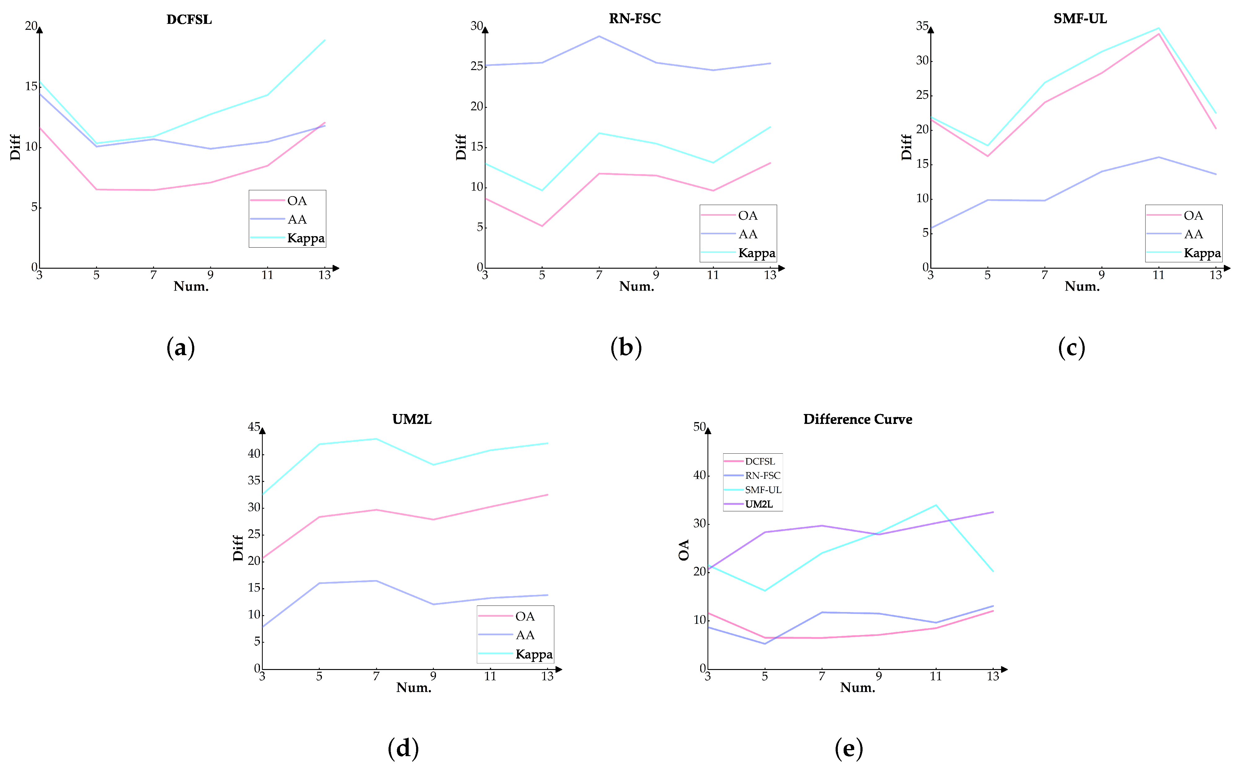
With the continuous sampling strategy, DCFSL achieves the highest OA with selected samples. DCFSL and RN-FSC also achieved higher classification accuracy than each model in Experiment 2 with continuous sampling. Therefore, FSL models exhibit excellent classification performance in some tasks with few samples. Although SMF-UL and UM2L demonstrate excellent classification accuracy using the random sampling strategy, their performance does not significantly surpass that of Experiment 2 using the continuous sampling strategy. Experimental results show that the SS-3D-CNN model in Experiment 2 is the least affected by information leakage when few samples are available, and its differences can be stabilized within 10%. However, even with random sampling, the OA of the model is only around 65%. In contrast, DCFSL and RN-FSC achieve better accuracy with spatially disjoint sampling methods, and maintain moderate differences between the two sampling strategies. While both unsupervised algorithms achieve better classification accuracy under the random sampling strategy, the OA does not improve significantly when spatially disjoint sampling strategies are used. As shown in Figure 13e, Comparing the difference of these models, FSL models show the excellently effective ability to mitigate information leakage.

In addition to evaluating the effectiveness of information leakage using the trends of the OA difference under different sampling strategies, AA and kappa are also used for evaluation in Table A4. As shown in Figure 13, the three evaluation indicators have the same overall trend and can be used to qualitatively describe the degree of information leakage. Kappa shows a highly similar trend to OA in different models, while AA shows a more gradual trend. This phenomenon may be caused by the class imbalance of the datasets. Specifically, for some class cases with a small number of samples, which have less spectral variation and a more concentrated distribution, spatially disjoint sampling can also contain most of the variation features. As a result, the accuracy of this class is less affected by changes in the number of training samples. Moreover, the accuracy of the class with a smaller number of samples receives better attention when calculating AA. Correspondingly, for classes with a large number of samples, the fraction of classification performance in computing AA decreases. In terms of evaluating the impact of information leakage, the contribution of each sample to the result should not be affected by the number of samples in the class of that sample. For example, the effect of information leakage due to random sampling is more pronounced for classes with a large number of samples. In the calculation of AA, the weights of all classes are the same, which weakens the performance of this effect and leads to a relatively gradual AA difference curve. This effect needs to be better reflected in the evaluation results. Considering this aspect, in this paper, we prefer to use OA as the metric to evaluate information leakage.

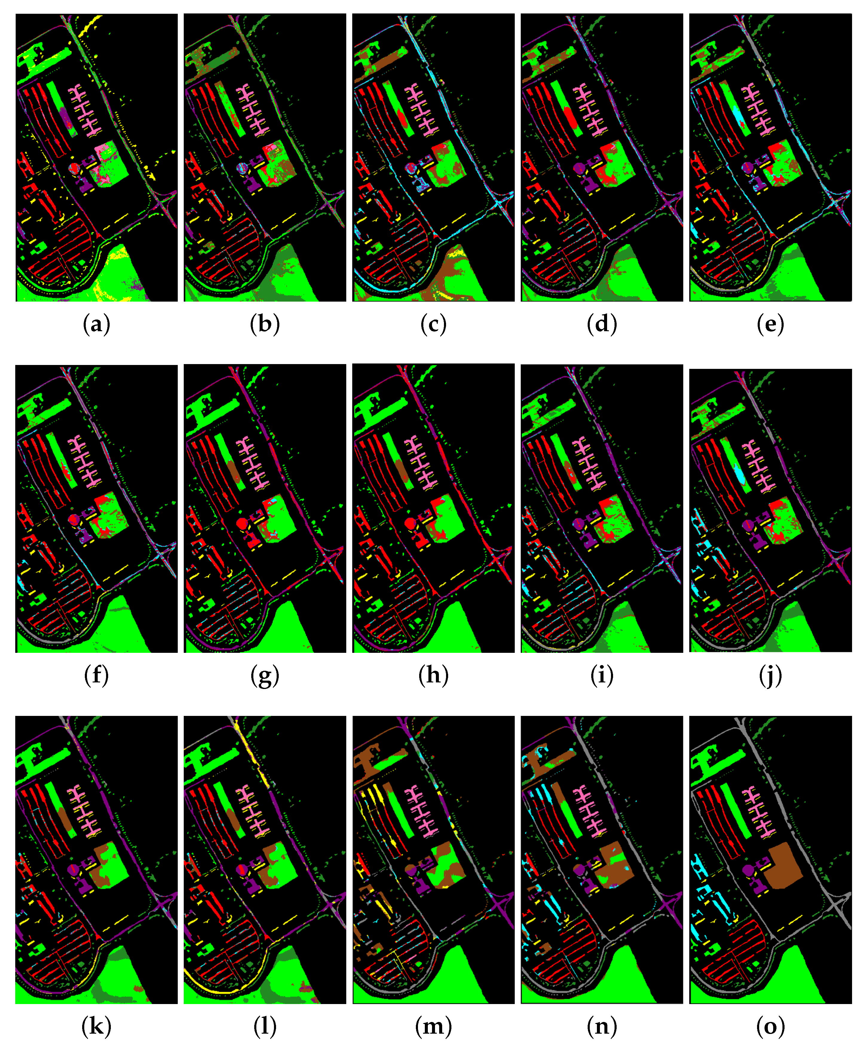
The four models used in this experiment all use cross-domain learning methods, and perform fine-tuning or feature extraction on the target domain during the cross-domain process. As shown in Figure 14, we compared the classification maps of the models from Experiment 2 and Experiment 3 under the conditions of using the UP dataset and spatially disjoint sampling strategy with 5 and 7 samples per class. The FSL models showed good classification performance for classes that are difficult for other models to recognize, such as bare soil and asphalt. FSL models, including DCFSL and RN-FSC, not only mitigate the issue of limited labeled samples and the subsequent low accuracy but also minimize the exposure of test set information during the training stage. Therefore, the models effectively mitigate information leakage under conditions that satisfy high classification accuracy.

4. Future Lines

While many deep learning-based HSI classification models have been proposed to achieve excellent classification accuracy under the random sampling strategy, there are still a few research works that use spatially disjoint sampling to evaluate the models. The high annotation cost and the lack of widely used homogeneous datasets are some of the objective reasons. As a result, most deep learning-based HSI classification models are trained and tested on a single HSI. Therefore, objective evaluation and practical application of deep learning models is an urgent direction for improvement in this field. Currently, the information leakage problem of HSI classification tasks can be intuitively reflected by spatially disjoint partitioning methods. However, relatively few models have been proposed specifically for such sampling methods and related problems. Most of the work in this paper is devoted to analyzing partial effective models for information leakage from existing models. Based on this, related future work can be considered in the following directions:

• As most current data augmentation methods obtain additional samples by processing labeled samples, the newly generated samples inevitably contain features of the original samples. For HSI data, spectra of the same ground-based object in different regions may have large variability. When a random sampling strategy is used, multiple spectral variants of the same class can be augmented to obtain an improvement in classification accuracy. However, the classification accuracy may be negatively affected under spatially disjoint sampling strategies. Samples of the same type selected in these strategies may have only a limited or even a single spectral variant type, which will cause the model to overfit the variants in these training samples. Therefore, it is possible to consider fusing some unlabeled samples with labeled samples. Methods such as hyperspectral unmixing and image edge segmentation are used to find objects of same classes at long spatial distances. These pixels can be fused with each other or added noise to obtain additional samples, allowing the model to learn different spectral variations;
• Recently, transformer networks have shown great potential in image processing. Several scholars have introduced vision transformer models into the field of hyperspectral classification and achieved advanced classification performance [92]. In HSI classification tasks, objects of the same class tend to be more concentrated in spatial locations. The self-attention mechanism used in transformers allows the network to focus more on the impact of each neighborhood pixel on the classification performance. Moreover, vision transformer models have better global feature extraction capabilities than CNN models. This ability to consider both neighbor and global information requires transformer models to introduce positional information at the input stage. From the information leakage perspective, most transformer models in classification tasks are identical to models, which do not remove test pixel information during training. Positional embedding may further exacerbate model overfitting to a single dataset. The combination of transformer models and graph structures can be considered as a future research direction. Specifically, some graph sample construction methods can strictly avoid the test information involved in training. The adjacency matrix in GCNs can be used to extract positional information;
• In practical applications, especially real-time remote sensing HSI classification, HSIs acquired by the same hyperspectral imaging platform usually share some features of homogeneous datasets. Examples are identical spatial resolution, spectral resolution or certain environmental conditions. The spectral response of objects in each pixel region will be more accurate with HSI spatial super-resolution or hyperspectral unmixing techniques, which mitigates the effect of object mixing on the spectrum. When the spectral variation is reduced, the samples obtained by the spatial disjoint sampling strategy have better generalization characteristics. To some extent, the problem of overfitting between datasets caused by information leakage is mitigated. Based on this, hyperspectral super-resolution technology and the construction of more accurate standard spectral libraries can be considered as future research directions;
• The current data augmentation methods struggle to achieve better performance of the model under spatial disjoint sampling strategies. Therefore they cannot steadily improve accuracy while reducing information leakage. The reason is that these data augmentation methods struggle to simulate the real spectral variation process. The task of super-resolution reconstruction based on deep learning is to simulate the degradation process of remote sensing images, and then use the original image as a supervision signal to construct a super-resolution model [93]. Inspired by this reconstruction technique, the variability process of spectra in HSI data can also be viewed as a degradation process. First, some bands in the original HSI that are likely to produce variation are identified based on prior knowledge, and then the degree of variation in that band is amplified as input to the model. The supervised signal is also the original HSI. The processed HSI is made closer to the original HSI data to construct the corresponding degradation model of the spectral variation process. Different from the HSI super-resolution, the process of amplifying spectral variation in this degradation model is more difficult to simulate real processes. The required prior knowledge may be affected by imaging platforms and environmental conditions in different regions;
• Most current deep learning-based HSI classification models need to be retrained when predicting different datasets. Based on this, several cross-domain learning methods have emerged. However, few models have been trained to directly classify various specifications of HSI without fine-tuning. The classification accuracy of these models also has room for improvement. This is a practical future research direction;
• In addition, the issue of information leakage in this field still requires the design of spatial autocorrelation evaluation indicators for hyperspectral occurrences. For example, mutual information can be used to obtain the degree of correlation between different samples. The reconstruction error of sparse representation can also be used to analyze the strength of correlations between samples. These methods can measure the independence of the test and training sets. In addition to spatially disjoint sampling strategies in HSI classification tasks, constructing perturbed samples can be an alternative approach to approximate homogeneous datasets. Based on this, it may be possible to add adversarial attacks to analyze the effectiveness of the model to mitigate information leakage.

5. Conclusions

This paper summarizes the existing problems in the field of deep learning-based HSI classification and provides a detailed analysis of the information leakage caused by the spatial autocorrelation and test information involved in training. In order to further illustrate the impact of this problem, the overfitting problem of HSI classification is divided into overfitting and overfitting between datasets. Based on the information leakage probability and expectation, the sample-related phase is divided into two aspects: reducing the number of training samples and using disjoint sampling strategies. In the feature extraction phase, some related models and learning paradigms are summarized, including FSL, unsupervised learning, GCNs. In particular, the reason why spatially disjoint sampling strategies are more objective is explained. The practical utility of such sampling is analyzed from the perspective of its approximation process for homogeneous datasets. Moreover, we experimentally demonstrate the impact of information leakage and the effectiveness of some related models and algorithms. Finally, several future research directions are suggested in this paper.

References

1. Wang, C.; Liu, B.; Liu, L.; Zhu, Y.; Hou, J.; Liu, P.; Li, X. A review of deep learning used in the hyperspectral image analysis for agriculture. Artif. Intell. Rev. 2021, 54, 5205–5253. [Google Scholar] [CrossRef]
2. Awad, M.M. An innovative intelligent system based on remote sensing and mathematical models for improving crop yield estimation. Inf. Process. Agric. 2019, 6, 316–325. [Google Scholar] [CrossRef]
3. Caballero, D.; Calvini, R.; Amigo, J.M. Hyperspectral imaging in crop fields: Precision agriculture. In Data Handling in Science and Technology; Elsevier: Amsterdam, The Netherlands, 2019; Volume 32, pp. 453–473. [Google Scholar]
4. Liu, B.; Liu, Z.; Men, S.; Li, Y.; Ding, Z.; He, J.; Zhao, Z. Underwater hyperspectral imaging technology and its applications for detecting and mapping the seafloor: A review. Sensors 2020, 20, 4962. [Google Scholar] [CrossRef] [PubMed]
5. Jay, S.; Guillaume, M. A novel maximum likelihood based method for mapping depth and water quality from hyperspectral remote-sensing data. Remote Sens. Environ. 2014, 147, 121–132. [Google Scholar] [CrossRef]
6. Gross, W.; Queck, F.; Vögtli, M.; Schreiner, S.; Kuester, J.; Böhler, J.; Mispelhorn, J.; Kneubühler, M.; Middelmann, W. A multi-temporal hyperspectral target detection experiment: Evaluation of military setups. In Proceedings of the Target and Background Signatures VII. SPIE, Online, 13–17 September 2021; Volume 11865, pp. 38–48. [Google Scholar]
7. Contreras Acosta, I.C.; Khodadadzadeh, M.; Gloaguen, R. Resolution enhancement for drill-core hyperspectral mineral mapping. Remote Sens. 2021, 13, 2296. [Google Scholar] [CrossRef]
8. Khan, U.; Paheding, S.; Elkin, C.P.; Devabhaktuni, V.K. Trends in deep learning for medical hyperspectral image analysis. IEEE Access 2021, 9, 79534–79548. [Google Scholar] [CrossRef]
9. Melgani, F.; Bruzzone, L. Classification of hyperspectral remote sensing images with support vector machines. IEEE Trans. Geosci. Remote Sens. 2004, 42, 1778–1790. [Google Scholar] [CrossRef] [Green Version]
10. Li, F.; Lu, H.; Zhang, P. An innovative multi-kernel learning algorithm for hyperspectral classification. Comput. Electr. Eng. 2019, 79, 106456. [Google Scholar] [CrossRef]
11. Liu, G.; Wang, L.; Liu, D.; Fei, L.; Yang, J. Hyperspectral Image Classification Based on Non-Parallel Support Vector Machine. Remote Sens. 2022, 14, 2447. [Google Scholar] [CrossRef]
12. Ham, J.; Chen, Y.; Crawford, M.M.; Ghosh, J. Investigation of the random forest framework for classification of hyperspectral data. IEEE Trans. Geosci. Remote Sens. 2005, 43, 492–501. [Google Scholar] [CrossRef] [Green Version]
13. Liu, W.; Fowler, J.E.; Zhao, C. Spatial logistic regression for support-vector classification of hyperspectral imagery. IEEE Geosci. Remote Sens. Lett. 2017, 14, 439–443. [Google Scholar] [CrossRef]
14. Wang, X. Kronecker factorization-based multinomial logistic regression for hyperspectral image classification. IEEE Geosci. Remote Sens. Lett. 2021, 19, 1–5. [Google Scholar] [CrossRef]
15. Khodadadzadeh, M.; Li, J.; Plaza, A.; Bioucas-Dias, J.M. A subspace-based multinomial logistic regression for hyperspectral image classification. IEEE Geosci. Remote Sens. Lett. 2014, 11, 2105–2109. [Google Scholar] [CrossRef]
16. Yu, H.; Gao, L.; Li, J.; Li, S.S.; Zhang, B.; Benediktsson, J.A. Spectral-spatial hyperspectral image classification using subspace-based support vector machines and adaptive Markov random fields. Remote Sens. 2016, 8, 355. [Google Scholar] [CrossRef] [Green Version]
17. Samat, A.; Gamba, P.; Abuduwaili, J.; Liu, S.; Miao, Z. Geodesic flow kernel support vector machine for hyperspectral image classification by unsupervised subspace feature transfer. Remote Sens. 2016, 8, 234. [Google Scholar] [CrossRef] [Green Version]
18. Zhang, Y.; Wang, Y.; Zhang, N.; Li, Z.; Zhao, Z.; Gao, Y.; Xu, D.; Ben, G. Orientation-First Strategy With Angle Attention Module for Rotated Object Detection in Remote Sensing Images. IEEE J. Sel. Top. Appl. Earth Obs. Remote Sens. 2022, 15, 8492–8505. [Google Scholar] [CrossRef]
19. Li, Z.; Wang, Y.; Zhang, N.; Zhang, Y.; Zhao, Z.; Xu, D.; Ben, G.; Gao, Y. Deep Learning-Based Object Detection Techniques for Remote Sensing Images: A Survey. Remote Sens. 2022, 14, 2385. [Google Scholar] [CrossRef]
20. Huang, B.; He, B.; Wu, L.; Guo, Z. Deep residual dual-attention network for super-resolution reconstruction of remote sensing images. Remote Sens. 2021, 13, 2784. [Google Scholar] [CrossRef]
21. Wen, D.; Huang, X.; Bovolo, F.; Li, J.; Ke, X.; Zhang, A.; Benediktsson, J.A. Change detection from very-high-spatial-resolution optical remote sensing images: Methods, applications, and future directions. IEEE Geosci. Remote Sens. Mag. 2021, 9, 68–101. [Google Scholar] [CrossRef]
22. Chen, Y.; Lin, Z.; Zhao, X.; Wang, G.; Gu, Y. Deep learning-based classification of hyperspectral data. IEEE J. Sel. Top. Appl. Earth Obs. Remote Sens. 2014, 7, 2094–2107. [Google Scholar] [CrossRef]
23. Chen, Y.; Zhu, L.; Ghamisi, P.; Jia, X.; Li, G.; Tang, L. Hyperspectral images classification with Gabor filtering and convolutional neural network. IEEE Geosci. Remote Sens. Lett. 2017, 14, 2355–2359. [Google Scholar] [CrossRef]
24. Zhu, J.; Fang, L.; Ghamisi, P. Deformable convolutional neural networks for hyperspectral image classification. IEEE Geosci. Remote Sens. Lett. 2018, 15, 1254–1258. [Google Scholar] [CrossRef]
25. Yue, J.; Zhao, W.; Mao, S.; Liu, H. Spectral–spatial classification of hyperspectral images using deep convolutional neural networks. Remote Sens. Lett. 2015, 6, 468–477. [Google Scholar] [CrossRef]
26. Li, Y.; Zhang, H.; Shen, Q. Spectral–spatial classification of hyperspectral imagery with 3D convolutional neural network. Remote Sens. 2017, 9, 67. [Google Scholar] [CrossRef] [Green Version]
27. Roy, S.K.; Manna, S.; Song, T.; Bruzzone, L. Attention-based adaptive spectral–spatial kernel ResNet for hyperspectral image classification. IEEE Trans. Geosci. Remote Sens. 2020, 59, 7831–7843. [Google Scholar] [CrossRef]
28. Pal, D.; Bundele, V.; Banerjee, B.; Jeppu, Y. SPN: Stable prototypical network for few-shot learning-based hyperspectral image classification. IEEE Geosci. Remote Sens. Lett. 2021, 19, 1–5. [Google Scholar] [CrossRef]
29. Bai, J.; Huang, S.; Xiao, Z.; Li, X.; Zhu, Y.; Regan, A.C.; Jiao, L. Few-shot hyperspectral image classification based on adaptive subspaces and feature transformation. IEEE Trans. Geosci. Remote Sens. 2022, 60, 1–17. [Google Scholar] [CrossRef]
30. Jia, S.; Jiang, S.; Lin, Z.; Li, N.; Xu, M.; Yu, S. A survey: Deep learning for hyperspectral image classification with few labeled samples. Neurocomputing 2021, 448, 179–204. [Google Scholar]
31. Molinier, M.; Kilpi, J. Avoiding overfitting when applying spectral-spatial deep learning methods on hyperspectral images with limited labels. In Proceedings of the IGARSS 2019-2019 IEEE International Geoscience and Remote Sensing Symposium, Yokohama, Japan, 28 July–2 August 2019; pp. 5049–5052. [Google Scholar]
32. Nalepa, J.; Myller, M.; Kawulok, M. Validating hyperspectral image segmentation. IEEE Geosci. Remote Sens. Lett. 2019, 16, 1264–1268. [Google Scholar] [CrossRef] [Green Version]
33. Liang, J.; Zhou, J.; Qian, Y.; Wen, L.; Bai, X.; Gao, Y. On the sampling strategy for evaluation of spectral-spatial methods in hyperspectral image classification. IEEE Trans. Geosci. Remote Sens. 2016, 55, 862–880. [Google Scholar] [CrossRef] [Green Version]
34. Zhou, J.; Liang, J.; Qian, Y.; Gao, Y.; Tong, L. On the sampling strategies for evaluation of joint spectral-spatial information based classifiers. In Proceedings of the 2015 7th Workshop on Hyperspectral Image and Signal Processing: Evolution in Remote Sensing (WHISPERS), Tokyo, Japan, 2–5 June 2015; pp. 1–4. [Google Scholar]
35. Qu, L.; Zhu, X.; Zheng, J.; Zou, L. Triple-attention-based parallel network for hyperspectral image classification. Remote Sens. 2021, 13, 324. [Google Scholar] [CrossRef]
36. Audebert, N.; Le Saux, B.; Lefèvre, S. Deep learning for classification of hyperspectral data: A comparative review. IEEE Geosci. Remote Sens. Mag. 2019, 7, 159–173. [Google Scholar] [CrossRef] [Green Version]
37. Li, S.; Song, W.; Fang, L.; Chen, Y.; Ghamisi, P.; Benediktsson, J.A. Deep learning for hyperspectral image classification: An overview. IEEE Trans. Geosci. Remote Sens. 2019, 57, 6690–6709. [Google Scholar] [CrossRef] [Green Version]
38. Mei, S.; Ji, J.; Geng, Y.; Zhang, Z.; Li, X.; Du, Q. Unsupervised spatial–spectral feature learning by 3D convolutional autoencoder for hyperspectral classification. IEEE Trans. Geosci. Remote Sens. 2019, 57, 6808–6820. [Google Scholar] [CrossRef]
39. Mou, L.; Ghamisi, P.; Zhu, X.X. Unsupervised spectral–spatial feature learning via deep residual Conv–Deconv network for hyperspectral image classification. IEEE Trans. Geosci. Remote Sens. 2017, 56, 391–406. [Google Scholar] [CrossRef] [Green Version]
40. Li, G.; Ma, S.; Li, K.; Zhou, M.; Lin, L. Band selection for heterogeneity classification of hyperspectral transmission images based on multi-criteria ranking. Infrared Phys. Technol. 2022, 125, 104317. [Google Scholar] [CrossRef]
41. Moharram, M.A.; Sundaram, D.M. Dimensionality reduction strategies for land use land cover classification based on airborne hyperspectral imagery: A survey. Environ. Sci. Pollut. Res. 2023, 30, 5580–5602. [Google Scholar] [CrossRef] [PubMed]
42. Zhang, T.; Wang, J.; Zhang, E.; Yu, K.; Zhang, Y.; Peng, J. RMCNet: Random Multiscale Convolutional Network for Hyperspectral Image Classification. IEEE Geosci. Remote Sens. Lett. 2020, 18, 1826–1830. [Google Scholar] [CrossRef]
43. Zhang, T.; Shi, C.; Liao, D.; Wang, L. Deep spectral spatial inverted residual network for hyperspectral image classification. Remote Sens. 2021, 13, 4472. [Google Scholar] [CrossRef]
44. Thoreau, R.; Achard, V.; Risser, L.; Berthelot, B.; Briottet, X. Active learning for hyperspectral image classification: A comparative review. IEEE Geosci. Remote Sens. Mag. 2022, 10, 256–278. [Google Scholar] [CrossRef]
45. Friedl, M.; Woodcock, C.; Gopal, S.; Muchoney, D.; Strahler, A.; Barker-Schaaf, C. A note on procedures used for accuracy assessment in land cover maps derived from AVHRR data. Int. J. Remote Sens. 2000, 21, 1073–1077. [Google Scholar] [CrossRef]
46. Belward, A.; Lambin, E. Limitations to the identification of spatial structures from AVHRR data. Int. J. Remote Sens. 1990, 11, 921–927. [Google Scholar] [CrossRef]
47. Zhen, Z.; Quackenbush, L.J.; Stehman, S.V.; Zhang, L. Impact of training and validation sample selection on classification accuracy and accuracy assessment when using reference polygons in object-based classification. Int. J. Remote Sens. 2013, 34, 6914–6930. [Google Scholar] [CrossRef]
48. Paoletti, M.; Haut, J.; Plaza, J.; Plaza, A. Deep learning classifiers for hyperspectral imaging: A review. ISPRS J. Photogramm. Remote Sens. 2019, 158, 279–317. [Google Scholar] [CrossRef]
49. Zou, L.; Zhu, X.; Wu, C.; Liu, Y.; Qu, L. Spectral–Spatial exploration for hyperspectral image classification via the fusion of fully convolutional networks. IEEE J. Sel. Top. Appl. Earth Obs. Remote Sens. 2020, 13, 659–674. [Google Scholar] [CrossRef]
50. Xue, Z.; Zhou, Y.; Du, P. S3Net: Spectral–spatial Siamese network for few-shot hyperspectral image classification. IEEE Trans. Geosci. Remote Sens. 2022, 60, 1–19. [Google Scholar] [CrossRef]
51. He, L.; Li, J.; Liu, C.; Li, S. Recent advances on spectral–spatial hyperspectral image classification: An overview and new guidelines. IEEE Trans. Geosci. Remote Sens. 2017, 56, 1579–1597. [Google Scholar] [CrossRef]
52. Sun, Y.; Liu, B.; Yu, X.; Yu, A.; Gao, K.; Ding, L. Perceiving Spectral Variation: Unsupervised Spectrum Motion Feature Learning for Hyperspectral Image Classification. IEEE Trans. Geosci. Remote Sens. 2022, 60, 1–17. [Google Scholar] [CrossRef]
53. Cao, X.; Liu, Z.; Li, X.; Xiao, Q.; Feng, J.; Jiao, L. Nonoverlapped Sampling for Hyperspectral Imagery: Performance Evaluation and a Cotraining-Based Classification Strategy. IEEE Trans. Geosci. Remote Sens. 2021, 60, 1–14. [Google Scholar] [CrossRef]
54. Zhang, H.; Li, Y.; Zhang, Y.; Shen, Q. Spectral-spatial classification of hyperspectral imagery using a dual-channel convolutional neural network. Remote Sens. Lett. 2017, 8, 438–447. [Google Scholar] [CrossRef] [Green Version]
55. Zhang, M.; Li, W.; Du, Q. Diverse region-based CNN for hyperspectral image classification. IEEE Trans. Image Process. 2018, 27, 2623–2634. [Google Scholar] [CrossRef]
56. Li, W.; Chen, C.; Zhang, M.; Li, H.; Du, Q. Data augmentation for hyperspectral image classification with deep CNN. IEEE Geosci. Remote Sens. Lett. 2018, 16, 593–597. [Google Scholar] [CrossRef]
57. Gao, H.; Zhang, J.; Cao, X.; Chen, Z.; Zhang, Y.; Li, C. Dynamic data augmentation method for hyperspectral image classification based on Siamese structure. IEEE J. Sel. Top. Appl. Earth Obs. Remote Sens. 2021, 14, 8063–8076. [Google Scholar] [CrossRef]
58. Zhang, X.; Wang, Y.; Zhang, N.; Xu, D.; Luo, H.; Chen, B.; Ben, G. Spectral–spatial fractal residual convolutional neural network with data balance augmentation for hyperspectral classification. IEEE Trans. Geosci. Remote Sens. 2021, 59, 10473–10487. [Google Scholar] [CrossRef]
59. Shang, X.; Han, S.; Song, M. Iterative spatial-spectral training sample augmentation for effective hyperspectral image classification. IEEE Geosci. Remote Sens. Lett. 2021, 19, 1–5. [Google Scholar] [CrossRef]
60. Creswell, A.; White, T.; Dumoulin, V.; Arulkumaran, K.; Sengupta, B.; Bharath, A.A. Generative adversarial networks: An overview. IEEE Signal Process. Mag. 2018, 35, 53–65. [Google Scholar] [CrossRef] [Green Version]
61. Neagoe, V.E.; Diaconescu, P. CNN hyperspectral image classification using training sample augmentation with generative adversarial networks. In Proceedings of the 2020 13th International Conference on Communications (COMM), Bucharest, Romania, 18–20 June 2020; pp. 515–519. [Google Scholar]
62. Dam, T.; Anavatti, S.G.; Abbass, H.A. Mixture of spectral generative adversarial networks for imbalanced hyperspectral image classification. IEEE Geosci. Remote Sens. Lett. 2020, 19, 1–5. [Google Scholar] [CrossRef]
63. Liang, H.; Bao, W.; Shen, X.; Zhang, X. Spectral–spatial attention feature extraction for hyperspectral image classification based on generative adversarial network. IEEE J. Sel. Top. Appl. Earth Obs. Remote Sens. 2021, 14, 10017–10032. [Google Scholar] [CrossRef]
64. Wang, G.; Ren, P. Delving into classifying hyperspectral images via graphical adversarial learning. IEEE J. Sel. Top. Appl. Earth Obs. Remote Sens. 2020, 13, 2019–2031. [Google Scholar] [CrossRef]
65. Hänsch, R.; Ley, A.; Hellwich, O. Correct and still wrong: The relationship between sampling strategies and the estimation of the generalization error. In Proceedings of the 2017 IEEE International Geoscience and Remote Sensing Symposium (IGARSS), Worth, TX, USA, 23–28 July 2017; pp. 3672–3675. [Google Scholar]
66. Lange, J.; Cavallaro, G.; Götz, M.; Erlingsson, E.; Riedel, M. The influence of sampling methods on pixel-wise hyperspectral image classification with 3D convolutional neural networks. In Proceedings of the IGARSS 2018—2018 IEEE International Geoscience and Remote Sensing Symposium, Valencia, Spai, 22–27 July 2018; pp. 2087–2090. [Google Scholar]
67. Li, J.; Wang, H.; Zhang, A.; Liu, Y. Semantic Segmentation of Hyperspectral Remote Sensing Images Based on PSE-UNet Model. Sensors 2022, 22, 9678. [Google Scholar] [CrossRef]
68. Ronneberger, O.; Fischer, P.; Brox, T. U-net: Convolutional networks for biomedical image segmentation. In Proceedings of the Medical Image Computing and Computer-Assisted Intervention–MICCAI 2015: 18th International Conference, Munich, Germany, 5–9 October 2015; Proceedings, Part III 18. Springer: Berlin/Heidelberg, Germany, 2015; pp. 234–241. [Google Scholar]
69. Vaswani, A.; Shazeer, N.; Parmar, N.; Uszkoreit, J.; Jones, L.; Gomez, A.N.; Kaiser, Ł.; Polosukhin, I. Attention is all you need. Adv. Neural Inf. Process. Syst. 2017, 30. [Google Scholar] [CrossRef]
70. Hu, X.; Li, T.; Zhou, T.; Liu, Y.; Peng, Y. Contrastive learning based on transformer for hyperspectral image classification. Appl. Sci. 2021, 11, 8670. [Google Scholar] [CrossRef]
71. Li, J.; Li, X.; Cao, Z.; Zhao, L. ROBYOL: Random-Occlusion-Based BYOL for Hyperspectral Image Classification. IEEE Geosci. Remote Sens. Lett. 2022, 19, 1–5. [Google Scholar] [CrossRef]
72. Liu, Z.; Ma, L.; Du, Q. Class-wise distribution adaptation for unsupervised classification of hyperspectral remote sensing images. IEEE Trans. Geosci. Remote Sens. 2020, 59, 508–521. [Google Scholar] [CrossRef]
73. Gao, K.; Liu, B.; Yu, X.; Yu, A. Unsupervised meta learning with multiview constraints for hyperspectral image small sample set classification. IEEE Trans. Image Process. 2022, 31, 3449–3462. [Google Scholar] [CrossRef]
74. Fang, L.; Zhao, W.; He, N.; Zhu, J. Multiscale CNNs ensemble based self-learning for hyperspectral image classification. IEEE Geosci. Remote Sens. Lett. 2020, 17, 1593–1597. [Google Scholar] [CrossRef]
75. Zhao, J.; Ba, Z.; Cao, X.; Feng, J.; Jiao, L. Deep Mutual-Teaching for Hyperspectral Imagery Classification. IEEE Geosci. Remote Sens. Lett. 2022, 19, 1–5. [Google Scholar] [CrossRef]
76. Hong, D.; Gao, L.; Yao, J.; Zhang, B.; Plaza, A.; Chanussot, J. Graph convolutional networks for hyperspectral image classification. IEEE Trans. Geosci. Remote Sens. 2020, 59, 5966–5978. [Google Scholar] [CrossRef]
77. Sha, A.; Wang, B.; Wu, X.; Zhang, L. Semisupervised classification for hyperspectral images using graph attention networks. IEEE Geosci. Remote Sens. Lett. 2020, 18, 157–161. [Google Scholar] [CrossRef]
78. He, Z.; Xia, K.; Li, T.; Zu, B.; Yin, Z.; Zhang, J. A constrained graph-based semi-supervised algorithm combined with particle cooperation and competition for hyperspectral image classification. Remote Sens. 2021, 13, 193. [Google Scholar] [CrossRef]
79. Xi, B.; Li, J.; Li, Y.; Du, Q. Semi-supervised graph prototypical networks for hyperspectral image classification. In Proceedings of the 2021 IEEE International Geoscience and Remote Sensing Symposium IGARSS, Brussels, Belgium, 11–16 July 2021; pp. 2851–2854. [Google Scholar]
80. Cai, Y.; Zhang, Z.; Cai, Z.; Liu, X.; Jiang, X. Hypergraph-structured autoencoder for unsupervised and semisupervised classification of hyperspectral image. IEEE Geosci. Remote Sens. Lett. 2021, 19, 1–5. [Google Scholar] [CrossRef]
81. Tang, H.; Huang, Z.; Li, Y.; Zhang, L.; Xie, W. A Multiscale Spatial–Spectral Prototypical Network for Hyperspectral Image Few-Shot Classification. IEEE Geosci. Remote Sens. Lett. 2022, 19, 1–5. [Google Scholar] [CrossRef]
82. Sun, J.; Shen, X.; Sun, Q. Hyperspectral Image Few-Shot Classification Network Based on the Earth Mover’s Distance. IEEE Trans. Geosci. Remote Sens. 2022, 60, 1–14. [Google Scholar] [CrossRef]
83. Li, Z.; Liu, M.; Chen, Y.; Xu, Y.; Li, W.; Du, Q. Deep Cross-Domain Few-Shot Learning for Hyperspectral Image Classification. IEEE Trans. Geosci. Remote Sens. 2022, 60, 1–18. [Google Scholar] [CrossRef]
84. Gao, K.; Liu, B.; Yu, X.; Qin, J.; Zhang, P.; Tan, X. Deep relation network for hyperspectral image few-shot classification. Remote Sens. 2020, 12, 923. [Google Scholar] [CrossRef] [Green Version]
85. 2013 IEEE GRSS Image Analysis and Data Fusion Contest. Available online: http://www.grss-ieee.org/community/technical-committees/data-fusion/ (accessed on 13 July 2022).
86. Debes, C.; Merentitis, A.; Heremans, R.; Hahn, J.; Frangiadakis, N.; van Kasteren, T.; Liao, T.; Bellens, R.; Pižurica, A.; Gautama, S.; et al. Hyperspectral and LiDAR Data Fusion: Outcome of the 2013 GRSS Data Fusion Contest. IEEE J. Sel. Top. Appl. Earth Obs. Remote Sens. 2014, 7, 2405–2418. [Google Scholar] [CrossRef]
87. Chen, Y.; Jiang, H.; Li, C.; Jia, X.; Ghamisi, P. Deep feature extraction and classification of hyperspectral images based on convolutional neural networks. IEEE Trans. Geosci. Remote Sens. 2016, 54, 6232–6251. [Google Scholar] [CrossRef] [Green Version]
88. Hu, W.; Huang, Y.; Wei, L.; Zhang, F.; Li, H. Deep convolutional neural networks for hyperspectral image classification. J. Sens. 2015, 2015, 258619. [Google Scholar] [CrossRef] [Green Version]
89. Zhu, M.; Jiao, L.; Liu, F.; Yang, S.; Wang, J. Residual spectral–Spatial attention network for hyperspectral image classification. IEEE Trans. Geosci. Remote Sens. 2020, 59, 449–462. [Google Scholar] [CrossRef]
90. Yang, X.; Ye, Y.; Li, X.; Lau, R.Y.; Zhang, X.; Huang, X. Hyperspectral image classification with deep learning models. IEEE Trans. Geosci. Remote Sens. 2018, 56, 5408–5423. [Google Scholar] [CrossRef]
91. Hamida, A.B.; Benoit, A.; Lambert, P.; Amar, C.B. 3-D deep learning approach for remote sensing image classification. IEEE Trans. Geosci. Remote Sens. 2018, 56, 4420–4434. [Google Scholar] [CrossRef] [Green Version]
92. He, W.; Huang, W.; Liao, S.; Xu, Z.; Yan, J. CSiT: A Multiscale Vision Transformer for Hyperspectral Image Classification. IEEE J. Sel. Top. Appl. Earth Obs. Remote Sens. 2022, 60, 9266–9277. [Google Scholar] [CrossRef]
93. Zhang, N.; Wang, Y.; Zhang, X.; Xu, D.; Wang, X.; Ben, G.; Zhao, Z.; Li, Z. A multi-degradation aided method for unsupervised remote sensing image super resolution with convolution neural networks. IEEE Trans. Geosci. Remote Sens. 2020, 60, 1–14. [Google Scholar] [CrossRef]
Figure 1. Two sources of information leakage: (a) excessive similarity between training and test samples when adjacent; (b) test set information is directly involved in network training because the training samples may contain test pixels.
Remotesensing 15 03793 g001
Figure 2. Timeline of studies related to information leakage: from the proposal of spatial autocorrelation to current research advances.
Remotesensing 15 03793 g002
Figure 3. Datasets partitioning in different spectral variation regions used spatially disjoint sampling process and random sampling.
Remotesensing 15 03793 g003
Figure 4. The ground truth of spatially disjoint sampling strategy (continuous sampling strategy) and random sampling strategy: (a) training samples with random sampling strategy; (b) test samples with random sampling strategy; (c) training samples with disjoint sampling strategy; (d) test samples with disjoint sampling strategy.
Remotesensing 15 03793 g004
Figure 5. Algorithms and models to mitigate information leakage.
Remotesensing 15 03793 g005
Figure 6. Unexposed test samples and the conditions of exposure.
Remotesensing 15 03793 g006
Figure 7. Evaluation methods of information leakage, impact of different sampling methods, and generalization ability between homogeneous datasets.
Remotesensing 15 03793 g007
Figure 8. Basic principles and structure of SAE: (a) basic structure of AE; (b) a framework for HSI classification model based on SAE.
Remotesensing 15 03793 g008
Figure 9. Basic principles and structure of FSL.
Remotesensing 15 03793 g009
Figure 10. OA and difference for each CNN model under different datasets (UP and IP) and different sampling strategies (random sampling and disjoint sampling): (a) LR-1D-CNN; (b) D-1D-CNN; (c) RSSAN; (d) R-2D-CNN; (e) SS-3D-CNN; (f) D-3D-CNN.
Remotesensing 15 03793 g010
Figure 11. OA difference of the CNN models on the UP dataset.
Remotesensing 15 03793 g011
Figure 12. OA and difference curves of CNN models with few samples and data augmentation: (a) LR-1D-CNN with different sampling strategies; (b) R-2D-CNN with different sampling strategies; (c) SS-3D-CNN with different sampling strategies; (d) the difference curve of LR-1D-CNN; (e) the difference curve of R-2D-CNN; (f) the difference curve of SS-3D-CNN.
Remotesensing 15 03793 g012
Figure 13. Difference curves of FSL and unsupervised learning models with few samples: (a) DCFSL; (b) RN-FSC; (c) SMF-UL; (d) UM2L; (e) the OA difference curve of the models.
Remotesensing 15 03793 g013
Figure 14. Classification maps of the models under the conditions of using the UP dataset and spatially disjoint sampling strategy with 5 and 7 samples per class: (a,b) LR-1D–CNN; (c,d) R-2D-CNN; (e,f) SS-3D-CNN; (g,h) SMF-UL; (i,j) UM2L; (k,l) DCFSL; (m,n) RN-FSC; (o) GT.
Remotesensing 15 03793 g014