Article

Reconstruction of Human-Induced Forest Loss in China during 1900–2000

1
College of Urban and Environmental Sciences, Peking University, Beijing 100871, China
2
Key Laboratory for Earth Surface Processes of the Ministry of Education, Peking University, Beijing 100871, China
3
School of Resource and Environmental Sciences, Wuhan University, Wuhan 430079, China
4
State Key Laboratory of Earth Surface Processes and Resources Ecology, Beijing Normal University, Beijing 100875, China
*
Author to whom correspondence should be addressed.
Remote Sens. 2023, 15(15), 3831; https://doi.org/10.3390/rs15153831
Submission received: 7 May 2023 / Revised: 13 July 2023 / Accepted: 26 July 2023 / Published: 1 August 2023

Abstract

:
Forests not only are an essential resource for human society but also have a significant impact on the climate. With the development of remote sensing technology, some progress has been made in forest change monitoring. However, relatively little research has been conducted on historical forest dynamics. Estimating forest loss and its drivers during historical time periods remains a scientific pursuit. In this study, we reconstructed forest loss and its dominant drivers across China based on long time-series socioeconomic and environmental data using LightGBM classification and regression models. The models showed good performance in both 10-fold cross-validation and comparison with other datasets. The results indicate that from 1900 to 2000, forest loss mainly occurred in southern China, with a total loss area of 34.4 × 10⁴ km2. Additionally, there was significant spatial heterogeneity, showing a decreasing trend from east to west and from south to north. The forest loss in China can be divided into two stages: (1) the stable stage from 1900 to 1949; and (2) the fluctuating stage from 1950 to 1999. In the first stage, most of the forest loss was attributed to forestry (>80%), followed by commodity-driven deforestation. In the early stage of the development of the People’s Republic of China, forest loss showed an increasing trend. In the 1960s, the forest loss area decreased by 12.9% due to the stagnation of the economy. With the adoption of the reform and opening-up policy, the total forest loss area in China reached its peak value (6.4 × 10⁴ km2) during 1980–1989. The models also accurately captured the impact of urbanization and government policy in this period. This study not only provides an in-depth understanding of historical forest change in China, but also offers data and methodological references for the further study of human–nature interactions over the long term.

Graphical Abstract

1. Introduction

Forests affect the climate [1,2,3], ecology [4,5], and human well-being [6,7] through a wide range of biophysical processes, biochemical processes, and carbon cycling. As a critical carbon sink, the carbon storage per unit of forestland is approximately two to four times that of farmland or grassland [8], and forestland can absorb one-third of the carbon emissions from fossil energy combustion each year [9].
Government-led National Forest Inventories (NFIs) can provide systematic and accurate information on forest resources. The State Forestry and Grassland Administration of China has now conducted nine forest data inventories, covering the period 1949–2018, with data from fixed sample plots distributed across the country (the ninth forest inventory included 4.15 × 10⁵ sample plots, but data from these plots are not available to the public). In addition, remote sensing techniques can provide forest observation data with high spatial and temporal resolutions. The Food and Agriculture Organization of the United Nations (FAO) started to utilize high-resolution remote sensing data to conduct forest resources assessments (FRA) in 1990. With the advance in cloud computing technology, Hansen et al. [10] produced the first global forest change (GFC) dataset using long time-series Landsat data on the Google Earth Engine (GEE). However, national inventories and remote sensing data cannot be traced back to historical times. Moreover, differences in statistical methods, spatial resolutions, and forest definitions also lead to different results [11,12].
The reconstruction of historical land use/land cover (LULC), including that of forestland, is an important topic of previous studies. Historical maps provided a way to assess centuries of land cover change. In Poland, historical maps confirmed the stability of the forest cover in the Białowieża Primeval Forest in the last 200 years [13]. But historical maps are often discontinuous and difficult to obtain, requiring extensive contextual knowledge, which is time and labor intensive [14]. Based on deforestation probabilities, Esser [15] estimated forest change in Europe from 1000 to 1850. Kaplan et al. [16] developed a land suitability model for deforestation based on the relationship between population density and land reclamation and used it to reconstruct European forestland for approximately 1000 years prior to the Industrial Revolution. Based on high-resolution remote sensing data and historical archives, Tian et al. [17] produced an Indian LULC dataset (including farmland, forest, shrubs, wildland, and built-up areas) from 1880 to 2010 with a resolution of 5°. He et al. [18] and Yang et al. [19] reconstructed the historical forestland in China from 1700 to 2000 based on a land suitability assessment model and the maximum extent of human disturbance. Based on the assumption that current land cover patterns are similar to their historical distributions, Liu and Tian [20] reconstructed the spatial patterns of agricultural land, forests, and cities in China from 1700 to 2005. Leite et al. [21] produced Brazilian farmland, natural pasture, and planted rangeland land-use dataset for 1940–1995 by merging satellite imagery with census data.
These reconstructed data provide not only a reliable source for climate and ecology modeling but also a valuable reference for subsequent studies. However, there are still some limitations. Reconstructions based on land reclamation suitability usually do not take into account forest continuity. Additionally, they are prone to detect significant changes in historical forests in areas far from cultivated land, residential areas, or road networks [19]. Most current studies are created by deducting the potential forestland based on land reclamation suitability models. However, this approach does not consider the other human-induced drivers, which can lead to temporary or long-term loss of forestland, such as forestry or urbanization. It may lead to an intrinsic bias in the results based on land reclamation suitability.
The drivers of forest disturbance have also drawn the attention of scholars. Current research falls into two main categories: the classification of forest change types based on remote sensing data and the exploration of the relationship between forest change and socioeconomic factors. The FRA 2020 report shows an overall slowdown in global deforestation [22]. Curtis et al. [23] produced the first global forest loss driver dataset from 2000–2014 based on the GFC dataset, including both permanent and temporary loss types. But these studies lack attention to historical forest loss. Forest change is often related to countries’ development processes, which can be depicted by a series of socioeconomic variables. Imai et al. [24] studied the drivers of deforestation in Southeast Asia and found that forest accessibility, forest productivity, and population pressure have a direct effect on deforestation. The forest transition (FT) model provides a conceptual framework for understanding the underlying socioeconomic factors that lead to forest change [25], but it is not applicable in all countries [26]. Currently, there is a lack of quantitative research to test whether there is a general pattern of human-disturbed forests during national development processes and whether this disturbance can be accurately portrayed using historical proxy variables.
As an extension of traditional statistical models, machine learning has recently been used for forest degradation and loss reconstruction due to its excellent predictive performance. Some studies have used machine learning methods to identify forest change [10] and forest loss drivers [23,27]. However, current studies of historical forest reconstruction focus on the spatial distribution patterns of forests over specific time periods and lack attention to the patterns of forest loss drivers.
This study aims to reconstruct the historical human-induced forestland loss in China from 1900 to 2000. Light Gradient Boosting Machine (LightGBM) models were developed based on forest loss data, forest loss type data, and long time-series socioeconomic and environmental data from 2001 to 2014 with over two million training samples. Then, we evaluated the temporal and spatial variability in forest loss and its human-induced drivers in China from 1900 to 2000.

2. Materials and Methods
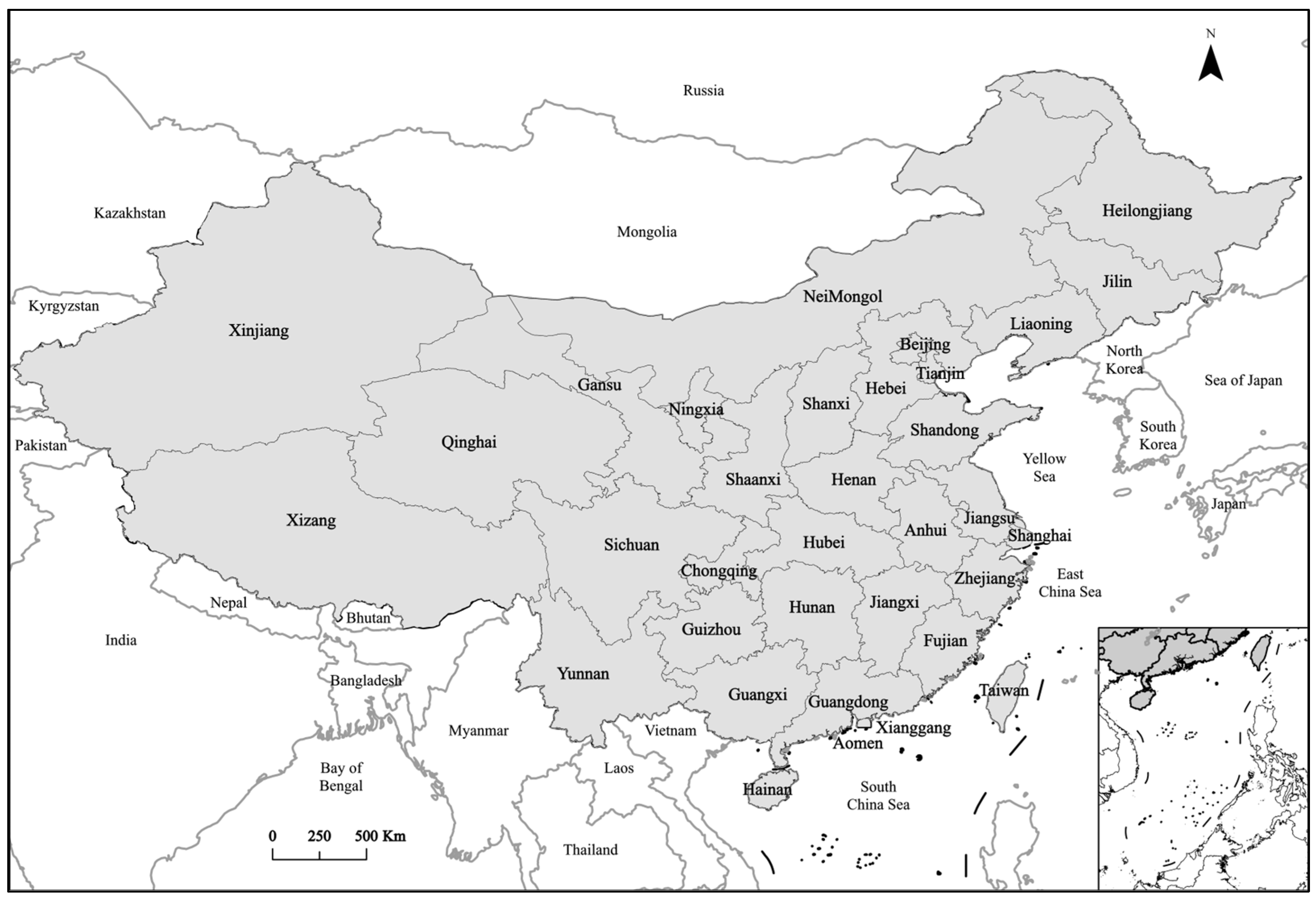
The framework of this study is shown in Figure 1. There are no forest monitoring datasets comparable to contemporary remote sensing products in the historical periods, but some socioeconomic and environmental indicators have long time-series records. Therefore, we used remote sensing forest monitoring datasets from 2001 to 2014 as the target values to model their relationships with the proxy indicators. The proxy indicators of the historical periods were then used as model inputs to obtain the historical forest loss raster data.

2.1. Study Area

This study focused on mainland China (excluding Taiwan, Hong Kong, and Macau), which plays an essential role in the world’s forest resources. Although China’s administrative boundary has changed a few times since 1900, the official statistical records were generally consistent after the founding of the People’s Republic of China in 1949. Because our reconstruction process is based on the grid scale, it is not affected by changes in administrative boundaries. However, the results show a change analysis based on provincial administrative regions. To be consistent with the current reality and enhance the practical significance, we use the data of China’s provincial administrative boundaries in 2000 provided by RESDC (https://www.resdc.cn/, accessed on 27 March 2022) as shown in Figure 2.

2.2. Data Sources

2.2.1. Forest Loss Data

The lack of high-resolution forest change datasets at the global scale and a uniform definition of forest cover and change have been major problems in related research. GFC data developed by Hansen et al. [10] quantified global forest decline and increase at a high spatial resolution for the first time. This dataset is open to the public and is of great importance for global forest monitoring. The data were produced on the GEE platform by processing Landsat data using supervised learning algorithms. The spatial resolution is 30 m and currently covers the period of 2001–2021. Trees were defined as all vegetation taller than 5 m in height. Forest loss was defined as a stand-replacement disturbance or the complete removal of tree cover canopy at the Landsat pixel scale. In this study, we used these data to calculate the area of forest loss within each study grid cell (10 km × 10 km).

2.2.2. Forest Loss Driver Data

Although global forest loss products have quantitatively described changes in forests at a fine scale, policymakers still need to distinguish between different types of forest loss to adjust their forest management policies. Based on the GFC dataset, Curtis et al. [23] identified the dominant drivers of forest loss and attributed tree cover loss that occurred over 15 years (2001–2015) to 5 specific disturbance types, including two types of permanent conversions and three types of temporary losses. For permanent conversions, there are (1) commodity-driven deforestation, defined as the long-term, permanent conversion of forests and shrublands to non-forestlands, such as agriculture, mining, or energy infrastructure; and (2) urbanization, defined as the conversion of forests and shrublands due to the expansion and intensification of existing urban centers. For temporary losses, there are (1) shifting agriculture, defined as the conversion of small- to medium-scale forests and scrublands to agricultural lands that are later abandoned and followed by forest regrowth; (2) forestry, defined as large-scale forestry operations that occur within managed forests with forest regrowth; and (3) wildfire, defined as the burning of forest vegetation resulting in large-scale forest loss without subsequent visible human conversion or agricultural activity.
To produce the data, the researchers first visually classified 4699 training sample cells using high-resolution Google Earth imagery and then developed a series of decision tree models based on multisource satellite data to predict dominant forest loss drivers in 10 km × 10 km grid cells globally. The evaluation of the models showed that the overall accuracy of the classification result is 89%. Since this dataset is consistent with the GFC, we overlaid it with the GFC to obtain the area of forest loss due to different dominant factors.

2.2.3. Multisource Socioeconomic and Environmental Features

This study incorporates several widely used data sources to construct a feature dataset for the classification of human-induced forest loss over historical periods. These data depict different aspects of the socioeconomic and environmental characteristics of the study grid cells. In addition to the indicators during the historical period (dynamic indicators), we obtained some static indicator data as a supplement. The static indicators may not change much over historical periods (e.g., elevation) or may be difficult to obtain (e.g., city accessibility), but can be used as background data. We also computed regional values and difference values for some of these indicators. Finally, a feature dataset of 113 indicators was formed (see Table A1).

2.2.4. HYDE 3.2 and LUH2-GCB Data

Two widely used global historical datasets, HYDE 3.2 (Historical Database of the Global Environment) and LUH2-GCB (Land-Use Harmonization 2 Update for the Global Carbon Budget), were utilized in this study to capture the characteristics of human social development processes in different study cells.
HYDE 3.2 is an internally consistent estimate of historical population and land use [30]. The data cover the period from 10 000 BCE to 2015 CE with a spatial resolution of 0.083 degrees. We resampled the data to 0.5 degrees during data extraction to obtain regional metrics. LUH2-GCB provides global annual gridded land use and land cover change data relating to agricultural expansion, deforestation, and timber harvesting. It is used by bookkeeping models for the global carbon budget (GCB) and in dynamic global vegetation models (DGVM) [31]. LUH2-GCB has a spatial resolution of 0.25 degrees, and contains fractional land-use states, transitions, and management practices from 850 to 2019. The data were resampled to 1 degree to obtain regional indicators.

2.2.5. Climate Data

Forest growth is closely related to climatic conditions. We extracted two indicators, precipitation and growing degree days, from the global bioclimatic indicator database [32]. This database is provided by the Copernicus Climate Change Service (C3S). The database covers a total of 78 indicators of bioclimatic variables for both terrestrial and marine environments. The spatial resolution is 0.5 degrees and covers the period from 1950 to 2100. In this paper, we used six models, ACCESS1-0, CSIRO-Mk3.6.0, GFDL-ESM2 M, HadGEM2-CC, IPSL-CM5A-MR and NorESM1-M, for multimodel averaging and extracted data for 1950, 2000 and 2020.

2.2.6. Gross Domestic Product Data

The demand for forest resources and the level of forestry production technology will change as the country develops. To characterize this feature, we used the historical GDP (gross domestic product) dataset developed by Geiger [28]. GDP is an important indicator of the country’s economic development. As GDP increases, the economic structure of the country changes. The share of forestry in GDP often decreases, and the advance of the industry will also improve the efficiency of forestry production. This dataset provides GDP data for 195 countries, including past observations (1850–2005) harmonized with future projections according to the shared socioeconomic pathways (2006–2100). The metrics were extracted from a gridded product of these data with a spatial resolution of 0.083 degrees, and regional metrics were extracted from a raster that was resampled to 0.5 degrees.

2.2.7. Other Data

In addition to the dynamic time-series data, a number of static indicators were added to the feature dataset. These indicators changed little over the study period or are available for only several years. Topography affects the conditions of forest growth and its potential for human disturbance. We extracted two indicators, elevation, and topographic relief, from the SRTM15+ product, with a spatial resolution of 0.083 degrees [33]. Cities are areas of intense human activity and are significant sites of the timber trade. Weiss et al. [29] evaluated global city accessibility and provided a high-resolution global gridded product. In this study, we extracted data that were resampled to 0.083 degrees and 0.5 degrees. Finally, we utilized two products based on satellite observations: the MODIS land cover product MCD12C1 [34] and the vegetation continuous fields (VCF) product MOD44B [35]. From these products, we extracted land cover indicators (resampled to 0.05 and 0.25 degrees) and tree cover indicators (resampled to 0.083 and 0.5 degrees). These two datasets are based on high-resolution satellite observations and accurately describe surface features. They can reflect the geographical heterogeneity of different regions, although they are available only for the modern period. Therefore, we used the dataset as background data for the study grid cells to complement the feature dataset.

2.3. Reconstruction Model

The light gradient boosting machine (LightGBM) is an algorithm framework proposed by Microsoft in 2017. It is an engineering implementation of the gradient boosting decision tree (GBDT) algorithm [36]. LightGBM can reduce the training time of a model with guaranteed accuracy and is well suited to handle large amounts of data.
In this study, multisource long time-series data from 1900 to 2015 were first preprocessed, and then a series of feature variables were extracted. The global forest loss driver data from 2001 to 2010 and from 2005 to 2014 were used as target values to train the forest loss driver classification model. Based on forest loss driver data and the GFC product, we extracted the loss areas corresponding to different loss drivers. These values were then used as target values for forest loss area regression models. Finally, we collected global forest loss area data, forest loss driver data, and proxy indicator data together to form a training dataset with a sample size of 2,178,163.
The classification and regression models were applied with the long time-series feature dataset to obtain forest loss driver and area predictions in 10-year intervals from 1900 to 2000. The forest loss drivers defined in the dataset include commodity-driven deforestation, urbanization, shifting agriculture, forestry, and wildfire (for detailed explanations, please refer to 2.2.2 Forest loss driver data). It is important to note that wildfire was beyond the scope of this study. Date preprocessing, construction and validation of the LightGBM model in this study were implemented via Python 3.6. Additionally, we used the Acrgis Pro 2.8 software to draw the maps in the results.

2.4. Model Evaluation

The 10-fold cross-validation approach was used to evaluate the performances of the classification and regression models. For the classification model, we calculated the accuracy index and produced a confusion matrix. The numbers on the diagonal line of the confusion matrix indicated the numbers of correctly predicted samples. We further calculated other model performance indices such as precision, recall, and F1-score. The indices are defined as follows:
a c c u r a c y = T P + T N T P + F P + F N + T N
p r e c i s i o n = T P T P + F P
r e c a l l = T P T P + F N
F 1 s c o r e = 2 × p r e c i s i o n × r e c a l l p r e c i s i o n + r e c a l l
where TP (true positive) denotes the number of correctly identified positive samples, TN (true negative) denotes the number of correctly identified negative samples, FP (false positive) denotes the number of incorrectly identified positive samples, and FN (false negative) denotes the number of incorrectly identified negative samples.
For the regression models, the coefficient of determination (R2), the root mean square error (RMSE), and the mean absolute error (MAE) were used:
R 2 = 1 i = 1 m y ^ i y i 2 i = 1 m y ¯ i y i 2
R M S E = 1 m i = 1 m y i y ^ i 2 ,
  M A E = 1 m i = 1 m y ^ i y i ,
where y i denotes the actual value of the sample i , y ^ i denotes the predicted value of the sample i , y ¯ i , denotes the mean value of all the samples, and m denotes the number of samples.

3. Results

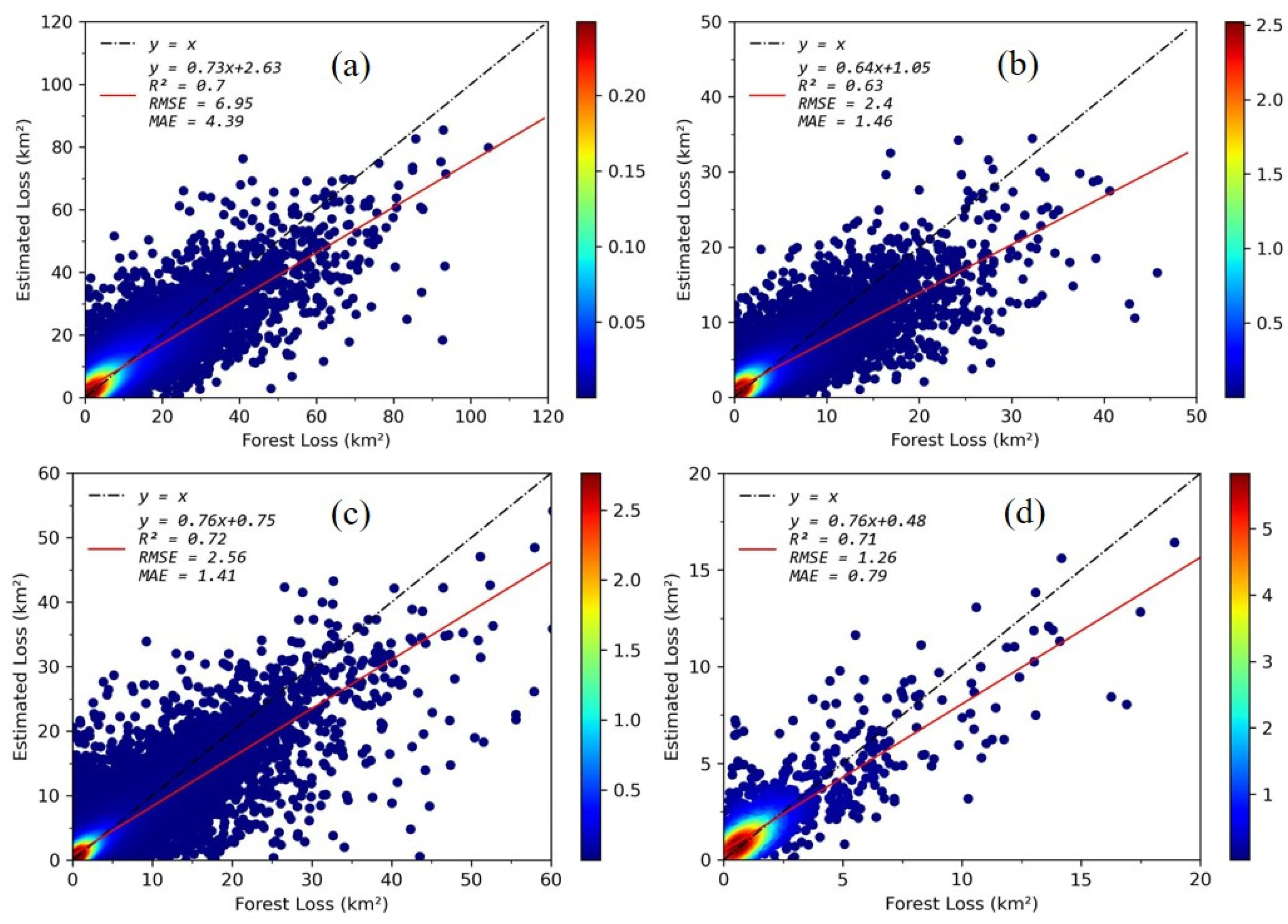
3.1. Model Evaluation Results

We first calculated the accuracy of the classification model. The classification model achieved an accuracy of 0.88, i.e., 88% of the predictions were correct, demonstrating that it had good prediction performance. The confusion matrix, shown in Figure 3, shows the detailed predictions of the model for different forest loss drivers. Furthermore, we calculated the precision, recall, and F1-score indices (shown in Table 1). Index values close to one indicate a good performance of this model in classification. As seen in Figure 3, the classification model has a strong prediction ability for no or minor loss and forestry types. This is mainly because the numbers of samples for these two variables are relatively large, which allows the model to obtain better generalization performance. The precision indices of commodity-driven deforestation, shifting agriculture, and urbanization types are 0.77, 0.79, and 0.61, respectively. The recall and F1-score of commodity-driven deforestation and shifting agriculture types are also higher than 0.7. The results show that the model also has relatively good performance in classifying these forest loss drivers.
For the regression models, we calculated the R2, RMSE, and MAE metrics. The results are shown in Figure 4. The RMSE and MAE of the model for commodity-driven deforestation are relatively high (RMSE = 6.95 km2, MAE = 4.39 km2). This may be attributed to the relatively small number of samples in this category. Additionally, there is usually a large fluctuation in forest loss area caused by such a driver, which makes it difficult to predict. The R2 metric of the model for shifting agriculture is relatively low (R2 = 0.63). This indicates that the model tends to underestimate the loss areas caused by such a driver. The regression model for urbanization achieved the best overall performance (R2 = 0.71, RMSE = 1.26 km2, MAE = 0.79 km2). This shows that the forest loss caused by urbanization is significant so that the model can be trained well. By comparing the linear regression lines of the four prediction models, it can be observed that the models tend to slightly overestimate in the low-value area and underestimate in the high-value area (both the slope k and intercept b are positive). In summary, all the models have relatively good generalization performance and can be applied to predict the loss areas caused by different dominant drivers.

3.2. Predictions of Forest Loss in China from 1900–2000

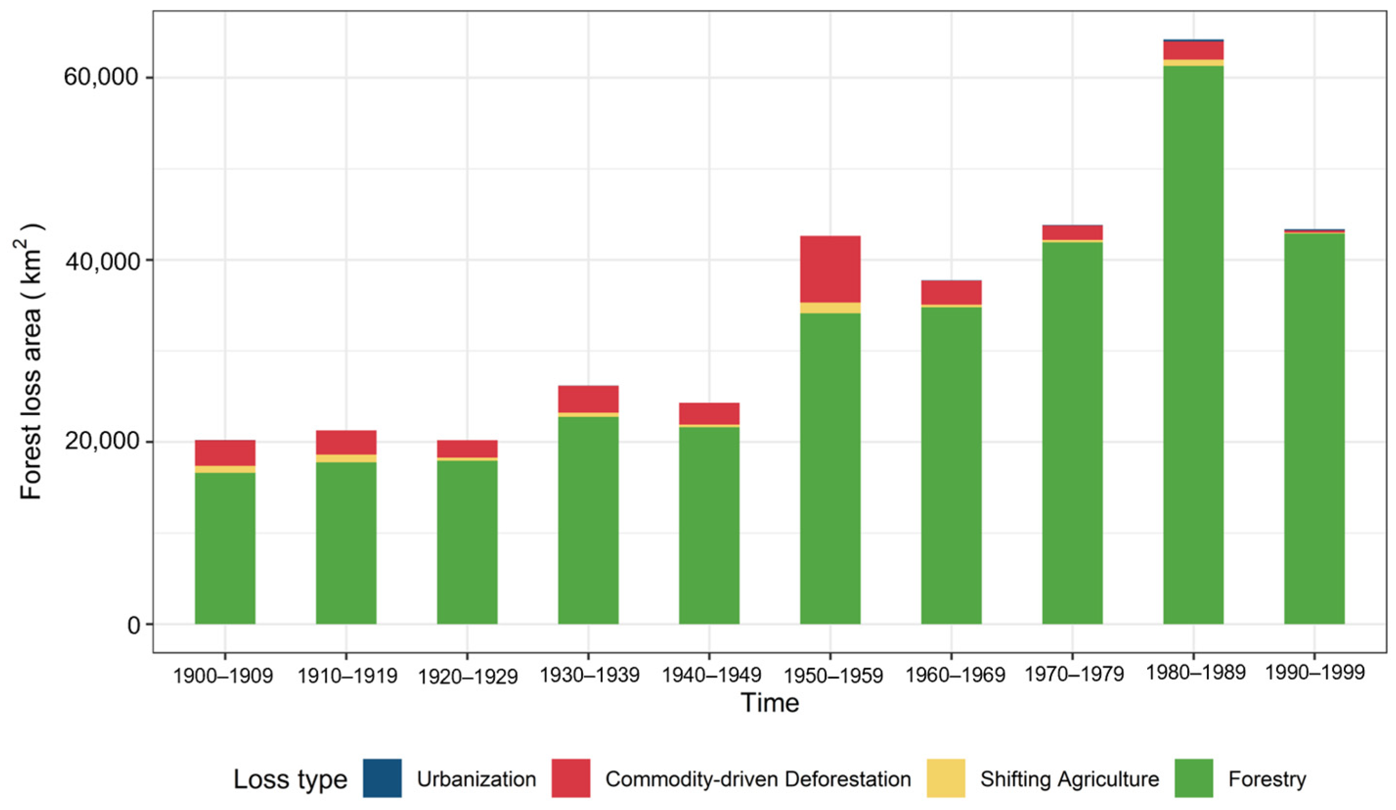
3.2.1. Forest Loss Area Caused by Different Drivers

After constructing the forest classification model and regression models, we predicted the forest loss within each decade during 1900–2000 using the long time-series feature dataset as input. The classification model was first applied to predict the dominant driver of forest loss in a study grid. Then the regression models were employed to predict the loss area corresponding to a specific driver. We calculated the area of each type of forest loss during the study period. As shown in Figure 5, the trend of forest loss from 1900 to 2000 can be roughly divided into two stages: (1) the stable stage from 1900 to 1949; and (2) the fluctuating stage from 1950 to 1999.
The trend of forest loss in China was relatively stable during 1900–1949. The area of forest loss per decade ranged from 2.02 × 10⁴ km2 to 2.61 × 10⁴ km2. Most of the forest loss is attributed to forestry (>80%), followed by commodity-driven deforestation (approximately 10%). During 1950–1959, a significant increase was observed in forest loss (42.9%). This period was the early stage of the development of the People’s Republic of China. The various industrial sectors of the country not only recovered rapidly but also showed a dramatic expansion. The GDP growth rate during this time period reached over 15%, and the population growth rate was maintained at over 20%. Rapid economic and demographic development led to a rapid rise in the country’s demand for forest resources. From 1950 to 1959, the forest loss led by commodity-driven deforestation increased by nearly 4 × 10³ km2, and forestry caused 3.4 × 10⁴ km2 of forest loss, mainly due to the Great Leap Forward campaign during 1958–1960. Starting from 1960, the change in forest loss showed an increasing trend followed by a decreasing trend. Forest loss due to forestry has increased significantly, and the effects of urbanization have gradually emerged. The forest loss due to commodity-driven deforestation and shifting agriculture declined during 1960–1979. The forest loss area reached its peak value during 1980–1989. The total forest loss area was 6.4 × 10⁴ km2, with forestry causing the largest loss (95.4%) and a significant increase in loss due to urbanization (3.2%). The main reason for this significant increase is the reform and opening-up policy adopted by the Chinese government. After a long period of low levels of growth, China’s economy started to develop at a fast rate, resulting in a sharp increase in the consumption of forest resources. In addition, due to the reform of the forestry management system in this period, forest resources were vigorously consumed in the absence of proper policy regulation. After 1990, with the further development of the country and the advancement of forest protection measures, the area of forest loss declined. In addition, we calculated the rate of change in forest loss at 20-year intervals for each provincial administrative region (Figure A1). From Figure A1, it is clear that after 1990, forest loss showed an overall decrease in all provinces, while before 1990, most areas showed an increase in forest loss, except for some provinces (such as Hubei, Xizang).

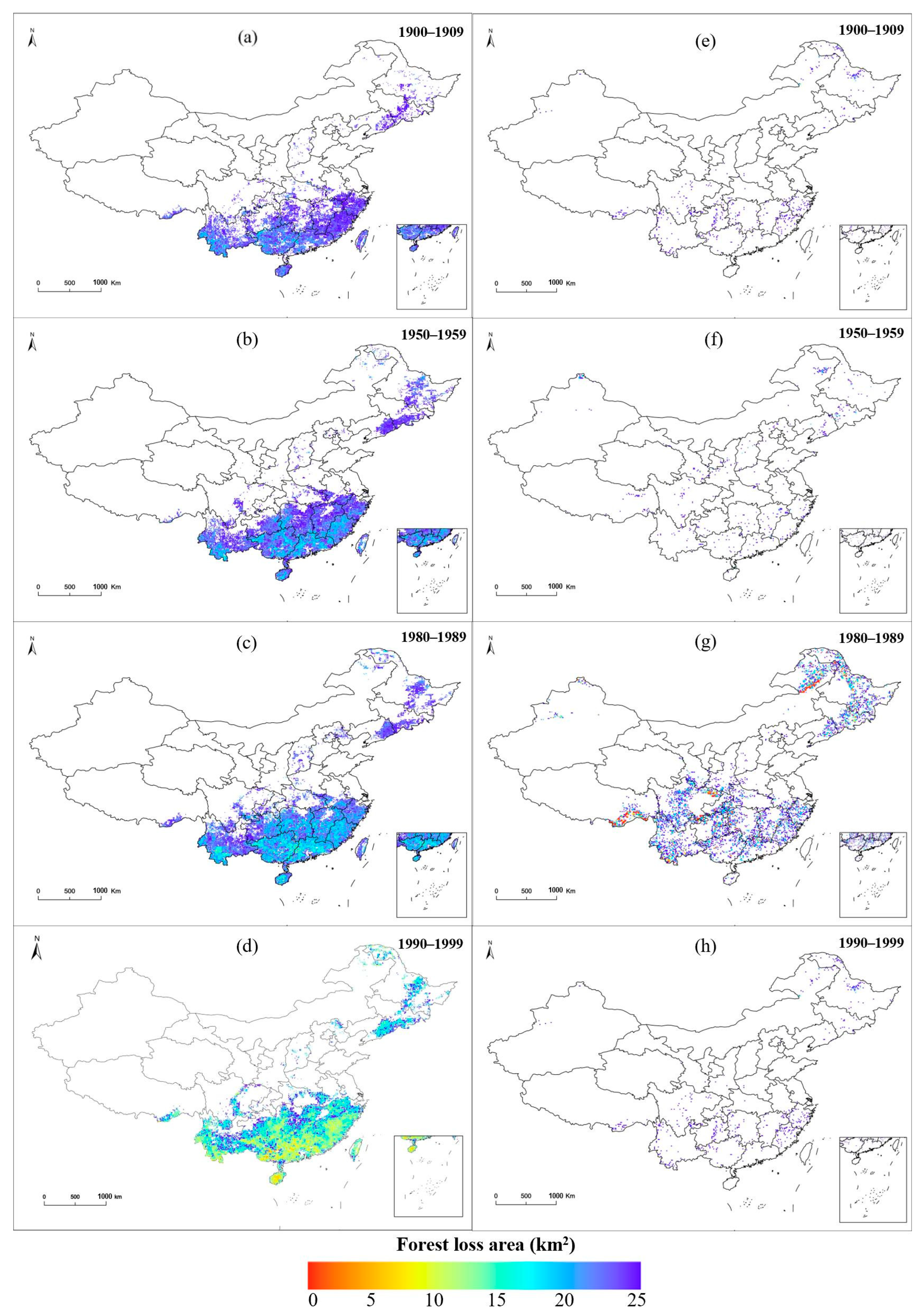
3.2.2. Spatial Distribution Patterns of Forest Loss

China’s forest resources are mainly distributed in the northeast and the southwest of the country, followed by the central south and the east. In contrast, northwestern, northern, and central China have relatively few forest resources. Using the prediction results, we produced maps of forest loss during 1900–2000 (Figure 6).
As shown in Figure 6, the most significant areas of forest loss in China were in the southern provinces of Guangxi, Guangdong, Fujian, Jiangxi, and Yunnan. In terms of spatial distribution, forest loss in China has an significant spatial heterogeneity, showing a decreasing trend from east to west and from south to north. Forestry was the dominant forest loss driver across the country, but the loss area in the northeast was relatively low compared to that in the southern provinces. Forest losses caused by commodity-driven deforestation were mainly distributed in southeastern Sichuan, northwestern Yunnan, southern and northeastern Guangxi, and southern Hainan and showed a decreasing trend. Large areas of forest loss led by shifting agriculture were mainly distributed in northwestern Yunnan.
Our models also accurately captured the impact of urbanization after the reform and opening-up of China. Forest losses caused by urbanization occurred mainly in 1980–2000 and were distributed near large urban agglomerations (the Pearl River Delta urban agglomeration, Sichuan–Chongqing urban agglomeration, and Chang-Zhu-Tan urban agglomeration). After 1990, the Chinese government implemented a series of conservation measures, including afforestation and reforestation. The area of forest loss led by commodity-driven deforestation and shifting agriculture declined significantly, and the overall forest loss also showed a downward trend.

4. Discussion

4.1. Comparison with Other Studies

To verify the effectiveness of our reconstruction results during the historical period, we compared the results of our study with existing relevant studies in this section. Although consistent in terms of overall trends, the existing statistical records and forest datasets based on remote sensing observations still differ significantly in quantity and are not comparable with each other [37]. Moreover, there are currently no unified and direct forest statistical records that cover the 20th century. More importantly, previous studies have mainly focused on forest cover patterns at specific time points rather than on forest loss over time periods due to various anthropogenic factors, as discussed in this study. Therefore, we selected several national forest datasets that cover limited time periods to test the results of this study.
The reconstructed results of He et al. [18] showed that the average annual reduction rate of forest area in China from 1900 to 1949 was 0.63%, which is similar to our result during the same time period (0.51%). The difference in the results is mainly because the reconstructed forest loss in our study is human-induced, excluding forest losses caused by natural factors such as wildfires or forest pests and diseases. The deforestation rate is defined as the percentage of forest area lost due to human influence, which can be obtained from national forest inventories. Because of the discontinuity of the NFIs, it is difficult to calculate the forest deforestation rate by year. Therefore, each time period is often used as the unit of calculation. In Li’s [38] study, there was a fluctuating upward trend after 1950, with the lowest rate of 1.4% during 1960–1969. The highest deforestation rate (3.16%) was recorded during 1980–1999, with other periods remaining at 2–3%. Figure 7 shows that our results have a similar overall trend. Another valuable data source is FAO’s historical statistics. We extracted the roundwood production data during 1960–1999 as shown in Figure 7. There was a continuous increase in roundwood production during 1960–1989 and a decline during 1990–1999. This is also consistent with the trend obtained in our study.
Few existing datasets on historical land use change fully account for gross change except for the HILDA+ dataset. So, we compared our gross forest loss data with the spatial distribution of HILDA+. The HILDA+ dataset was harmonized from FAO statistics and remote sensing images [39]. The reconstruction of LUCC was based on the potential allocation of probability maps derived from gridded images in HILDA+ during 1900–2019. We performed spatial comparisons of the reconstructed forest transition with HILDA+ in the years 1990, 1950, 1980, and 1990 (Figure 8). Spatially, the forest loss distribution has a stronger consistency in the 1980s, and the HILDA+ dataset has significantly smaller forest loss in other years than our study and the statistical data. According to China Statistical Yearbook, the net forest loss in China from 1990 to 1999 was about 7304.67 km2, which was much larger than the HILDA+ results (2016 km2). In the reconstruction process, the HILDA+ dataset may be based on the FAO net forest loss data and extended to the past hundred years, with 2015 as the base year. This means that FAO data would heavily influence it. It has been noted that the large change in FAO cropland statistics was damped by the limiting threshold applied, resulting in the overestimation of cropland before the 1980s [40]. Forests are often contrary to changes in cropland data, which may have contributed to the apparent underestimation of the area of forest loss by HILDA+. In addition, HILDA+ is focused on global reconstructions, which may have deviations when applied in regions. In summary, our reconstruction may better reflect the gross forest loss change in China over the past century.

4.2. Spatiotemporal Changes in Forest Loss during Historical Periods

In terms of spatial distribution, forest loss in China has a significant spatial heterogeneity, showing a decreasing trend from east to west and from south to north. This decreasing trend is closely related to the more abundant forest resources in southern and eastern China. The 6th NFI [41] in China shows that the forest cover in the east region was 34.27%, 27.12% in the central region, and only 12.54% in the western region. Statistics also show that nine provinces in China had more than 40% forest cover in the late 1990s, and all of them are located in the southern provinces. Additionally, the more developed economic status of the cities along the southeast coast is another cause of spatial heterogeneity. Imai et al. [24] highlighted that deforestation might be accelerated in regions undergoing societal transition. With the development of the economy, the demand for forest resources will also rise. Meanwhile, farmers tend to seek other kinds of jobs in this process, which results in the abandonment of marginal cropland [42] and a decrease in forest loss due to commercial agriculture [43]. As the pioneer of China’s reform and opening up, the southeastern coastal region has experienced rapid economic development, and forest loss due to urbanization in this region has shown a significant increase.
With regard to the temporal changes of forest loss, our study also validated the forest transition (FT) concept in China over the past century. The FT concept describes the change in national forest area from declining to increasing with the development of the economy [25]. According to the FT concept, the demand for forest resources and the level of forestry production technology will change as a country develops. Mather [44] proposed that the forest transition in China occurred around 1980, based on data from Fang et al. [45] and FAO statistics on agriculture and forestry. Li and Zhao [46] suggested that it is more reliable to date the forest transition in China to 1980–1989 based on national forest inventory data. This is consistent with the turning point obtained in this study. Our results also revealed that commodity-driven deforestation decreased from 1569.9 km2 (3.58%) to 234.7 km2 (0.54%) around the turning point, while urbanization increased from 64. 2 km2 (1.47%) to 142.1 km2 (3.05%). It suggests that the “economic development path” [43] may explain the FT transition in China.
Lambin and Meyfroidt [47] suggested that government policies have significantly impacted forests, especially in Asian countries. China, in particular, has seen both positive and negative effects of these policies on its forest resources over the past century. According to our results, the negative impacts mainly occurred during the periods of 1950–1969 and 1980–1989. During the Great Leap Forward movement from 1958 to 1960, forest loss skyrocketed due to commodity-driven deforestation. Around 60 million people were sent to the mountains to cut down trees and make charcoal, resulting in severe damage to China’s forest resources. According to statistics, the planned timber consumption alone reached 3.657 × 10⁷ m3 during this period, an increase of 45% compared to that in 1957 [38]. Additionally, the natural disasters (1959–1961) and later the Cultural Revolution (1966–1976) caused the slow development of the economy. During the early 1980s, the forestry management system was also transformed, but without the necessary support facilities, it led to the unsustainable consumption of forest resources. This issue was especially prevalent in the collective forest areas in the southern part of the country. As environmental concerns grew more pressing, the government became more focused on protecting the forests [48]. One positive outcome of these efforts was a relatively significant decrease in forest loss from 1990 to 2000, which was supported by ecological protection policies like “grain for green”.

4.3. Applications and Limitations of This Study

All parties to the Paris Agreement committed to achieving a balance between anthropogenic carbon emissions and ecosystem carbon sinks by the second half of this century. The Chinese government also pledged to peak its CO2 emissions around 2030. As forests are an essential carbon sink, accurately quantifying their temporal and spatial changes is crucial. This study reconstructed a high-precision dataset of anthropogenic disturbances in Chinese forests, reflecting the temporal and spatial patterns of human activities such as deforestation throughout history. It is significant for a deeper understanding of the long-term effects of human forest disturbances on global carbon, water, and climate cycles. It can also provide technical support for effective forest management and enhancing forest carbon sinks. Additionally, it can help quantitatively study the impact of anthropogenic disturbances on forest carbon storage in China over the past century, providing scientific data support for the country’s participation in international climate change negotiations and implementation of climate change measures. Additionally, forest loss worldwide is a major factor in landscape structural change [49]. Forest loss and caused fragmentation can have a broad range of effects on population survival, ecological interactions, and biodiversity [50]. Our study can also provide a data source for historical habitat loss research.
Although this study contributes to the understanding of historical forest loss and its drivers, there are some limitations to this study. Multisource remote sensing monitoring data were used in our study to ensure a sufficient training dataset for reconstruction. This may lead to the inconsistency of spatial resolutions of the input datasets. To minimize the impact of this problem, we resampled all the datasets to 10 km grids. We built a training dataset with a large sample size and utilized the LightGBM model, which has a strong anti-noise ability [51]. Additionally, the spatial resolution is relatively coarse (10 km), which may cause the uncertainty introduced by the heterogeneity within each grid cell. The coarse spatial resolution is a common problem in historical LULC reconstructions, considering the limitations in the availability of historical data sources. Moreover, it also makes it difficult to validate the reconstruction results at a finer spatial scale.

5. Conclusions

In this study, machine learning models were constructed to explore the relationship between human-induced forest loss and various environmental and socioeconomic variables. Based on the historical long time-series remote sensing dataset, we classified the drivers of human-induced forest losses and predicted the specific loss areas in 10-year intervals from 1900 to 2000. The accuracy of the classification model is 0.88. For the regression models, the R2 of the models of forest loss caused by commodity-driven deforestation, shifting agriculture, forestry, and urbanization are 0.70, 0.63, 0.72, and 0.71, respectively. When compared with other studies, our estimates share similar overall trends with them. These results show that the reconstruction models have good prediction performance.
The results indicate that from 1900 to 2000, forest loss mainly occurred in southern China, with a total loss area of 34.4 × 10⁴ km2. The distribution of forest loss has a significant spatial heterogeneity, showing a decreasing trend from east to west and from south to north. This decreasing trend was also related to the richer forests and more developed economic status of the cities along the southeast coast. Forestry was the main cause of forest loss, accounting for more than 80%. Forest loss caused by commodity-driven deforestation was mainly distributed in southeastern Sichuan, northwestern Yunnan, southern and northeastern Guangxi, and southern Hainan. Large areas of forest loss led by shifting agriculture were mainly distributed in northwestern Yunnan.
Most previous studies have investigated the distribution of forests at particular historical time points. In this study, we explored the dynamics of forest loss and what factors were driving such loss. Previous studies tend to focus on permanent forest loss drivers such as land reclamation. However, temporary forest loss, such as forestry practices, also has a significant impact on the carbon cycle. As our results revealed, forestry accounted for more than 80% of forest loss during the past century. Moreover, our study also captured the influence of the economic development path and government policy. The results validated the theories of the FT concept with empirical data from China. In summary, this study not only offers data and methodological references for forestland reconstructions but also provides a deeper understanding of human–nature interactions over the long term.

Author Contributions

Y.Z. (Yanwen Zhang): Methodology, Software, Validation, Writing—original draft. J.D.: Conceptualization, Methodology, Software, Writing—original draft. Y.W.: Software. Y.Z. (Yajuan Zhang): Data curation. Y.L. (Yinglu Liu): Data curation. L.Z.: Data curation. M.A.: Data curation. T.W.: Data curation. W.H.: Writing—review and editing. Y.L. (Yan Li): Writing—review and editing. S.L.: Writing—review and editing, Supervision, Project administration, Funding acquisition. All authors have read and agreed to the published version of the manuscript.

Funding

This work was supported by the National Key Research and Development Program of China (No. 2019YFA0606602) and the National Natural Science Foundation of China (No. 42230506).

Data Availability Statement

Not applicable.

Conflicts of Interest

The authors declare no conflict of interest.

Appendix A

Table A1. Feature dataset. Listed in the table are the original spatial resolutions of the datasets, which may be resampled to extract the indicators.
NameMeaningImplicationSourceResolution
primf, primn, prim (_regional, _diff)ratio of forested primary land, non-forested primary land, and primary landabundance of forest resourcesLUH2-GCB0.25°
secdn, secdf, secd (_regional, _diff)ratio of potentially forested secondary land, potentially non-forested secondary land, and secondary landabundance of forest resourcesLUH2-GCB0.25°
c3ann, c3per, c4ann, c4per, crop (_regional, _diff)ratio of C3 annual crops, C3 perennial crops, C4 annual crops, C4 perennial crops, and cropspressure on forests from agricultureLUH2-GCB0.25°
pastr (_regional, _diff)ratio of managed pasturepressure on forests from livestock farmingLUH2-GCB0.25°
range (_regional, _diff)ratio of rangelandpressure on forests from livestock farmingLUH2-GCB0.25°
urban (_regional, _diff)ratio of urban landpressure on forests from general human demandLUH2-GCB0.25°
GDDgrowing degree dayssuitability of forest growthGlobal bioclimatic indicators database0.5°
preprecipitationsuitability of forest growthGlobal bioclimatic indicators database0.5°
pop (_regional, _diff)populationpressure on forests from general human demandHYDE 3.20.0833°
land_use(_regional)land usegeneral human impactHYDE 3.20.0833°
GDP (_regional, _diff)gross domestic productionregional development conditionGlobal GDP time-series dataset0.0833°
land_cover (_regional)land covergeneral human impactMCD12C10.05°
tree_cover (_regional)tree coverabundance of forest resourcesMOD44B250 m
elevationelevationforest growth suitability and potential for human disturbanceSRTM15+0.00417°
reliefreliefforest growth suitability and potential for human disturbanceSRTM15+0.00417°
city_access (_regional)accessibility to citieswood trade accessibility, intensity of human activityGlobal city accessibility map0.00833°
Difference values (with the suffix “_diff”) refer to the difference between the starting and ending years for every 10-year interval. Regional values (with the suffix “_regional”) refer to data resampled to a coarser spatial resolution. Since the resampling process considers neighborhood pixels, these indicators can reflect the average situation over a larger area.
Figure A1. Rates of change in forest loss at 20-year intervals from 1900 to 2000 by provincial administrative regions in China. Rates of change = (previous period forest loss − next period forest loss)/previous period forest loss × 100%, “-” refer to the null value. Pink grids represent an increase in forest loss and green grids represent a decrease in forest loss.
Remotesensing 15 03831 g0a1

References

  1. Devaraju, N.; Bala, G.; Modak, A. Effects of large-scale deforestation on precipitation in the monsoon regions: Remote versus local effects. Proc. Natl. Acad. Sci. USA 2015, 112, 3257–3262. [Google Scholar] [CrossRef]
  2. Lee, X.; Goulden, M.L.; Hollinger, D.Y.; Barr, A.; Black, T.A.; Bohrer, G.; Bracho, R.; Drake, B.; Goldstein, A.; Gu, L.; et al. Observed increase in local cooling effect of deforestation at higher latitudes. Nature 2011, 479, 384–387. [Google Scholar] [CrossRef] [PubMed] [Green Version]
  3. Martinich, J.; Crimmins, A.; Beach, R.H.; Thomson, A.; McFarland, J. Focus on agriculture and forestry benefits of reducing climate change impacts. Environ. Res. Lett. 2017, 12, 060301. [Google Scholar] [CrossRef] [Green Version]
  4. Hua, F.; Wang, X.; Zheng, X.; Fisher, B.; Wang, L.; Zhu, J.; Tang, Y.; Yu, D.W.; Wilcove, D.S. Opportunities for biodiversity gains under the world’s largest reforestation programme. Nat. Commun. 2016, 7, 12717. [Google Scholar] [CrossRef] [Green Version]
  5. Veldkamp, E.; Schmidt, M.; Powers, J.S.; Corre, M.D. Deforestation and reforestation impacts on soils in the tropics. Nat. Rev. Earth Environ. 2020, 1, 590–605. [Google Scholar] [CrossRef]
  6. Bonan Gordon, B. Forests and Climate Change: Forcings, Feedbacks, and the Climate Benefits of Forests. Science 2008, 320, 1444–1449. [Google Scholar] [CrossRef] [Green Version]
  7. Wolff, N.H.; Zeppetello, L.R.V.; Parsons, L.A.; Aggraeni, I.; Battisti, D.S.; Ebi, K.L.; Game, E.T.; Kroeger, T.; Masuda, Y.J.; Spector, J.T. The effect of deforestation and climate change on all-cause mortality and unsafe work conditions due to heat exposure in Berau, Indonesia: A modelling study. Lancet Planet. Health 2021, 5, e882–e892. [Google Scholar] [CrossRef] [PubMed]
  8. Houghton, R.A.; Hobbie, J.E.; Melillo, J.M.; Moore, B.; Peterson, B.J.; Shaver, G.R.; Woodwell, G.M. Changes in the Carbon Content of Terrestrial Biota and Soils between 1860 and 1980: A Net Release of CO’2 to the Atmosphere. Ecol. Monogr. 1983, 53, 235–262. [Google Scholar] [CrossRef]
  9. Friedlingstein, P.; O’Sullivan, M.; Jones, M.W.; Andrew, R.M.; Hauck, J.; Olsen, A.; Peters, G.P.; Peters, W.; Pongratz, J.; Sitch, S.; et al. Global Carbon Budget 2020. Earth Syst. Sci. Data 2020, 12, 3269–3340. [Google Scholar] [CrossRef]
  10. Hansen, M.C.; Potapov, P.V.; Moore, R.; Hancher, M.; Turubanova, S.A.; Tyukavina, A.; Thau, D.; Stehman, S.V.; Goetz, S.J.; Loveland, T.R.; et al. High-Resolution Global Maps of 21st-Century Forest Cover Change. Science 2013, 342, 850–853. [Google Scholar] [CrossRef] [Green Version]
  11. Wang, H.; Lü, Z.; Gu, L.; Wen, C. Observations of China’s forest change (2000–2013) based on Global Forest Watch dataset. Biodivers. Sci. 2015, 23, 575–582. [Google Scholar] [CrossRef]
  12. Li, Y.; Sulla-Menashe, D.; Motesharrei, S.; Song, X.-P.; Kalnay, E.; Ying, Q.; Li, S.; Ma, Z. Inconsistent estimates of forest cover change in China between 2000 and 2013 from multiple datasets: Differences in parameters, spatial resolution, and definitions. Sci. Rep. 2017, 7, 8748. [Google Scholar] [CrossRef]
  13. Mikusinska, A.; Zawadzka, B.; Samojlik, T.; Jędrzejewska, B.; Mikusiński, G. Quantifying landscape change during the last two centuries in Białowieża Primeval Forest. Appl. Veg. Sci. 2013, 16, 217–226. [Google Scholar] [CrossRef]
  14. Kaim, D.; Kozak, J.; Kolecka, N.; Ziółkowska, E.; Ostafin, K.; Ostapowicz, K.; Gimmi, U.; Munteanu, C.; Radeloff, V.C. Broad scale forest cover reconstruction from historical topographic maps. Appl. Geogr. 2016, 67, 39–48. [Google Scholar] [CrossRef]
  15. Esser, G.; Lautenschlager, M. Estimating the change of carbon in the terrestrial biosphere from 18 000 BP to present using a carbon cycle model. Environ. Pollut. 1994, 83, 45–53. [Google Scholar] [CrossRef]
  16. Kaplan, J.O.; Krumhardt, K.M.; Zimmermann, N. The prehistoric and preindustrial deforestation of Europe. Quat. Sci. Rev. 2009, 28, 3016–3034. [Google Scholar] [CrossRef]
  17. Tian, H.; Banger, K.; Bo, T.; Dadhwal, V.K. History of land use in India during 1880–2010: Large-scale land transformations reconstructed from satellite data and historical archives. Glob. Planet. Chang. 2014, 121, 78–88. [Google Scholar] [CrossRef] [Green Version]
  18. He, F.; Li, S.; Zhang, X. A spatially explicit reconstruction of forest cover in China over 1700–2000. Glob. Planet. Chang. 2015, 131, 73–81. [Google Scholar] [CrossRef]
  19. Yang, X.; Jin, X.; Xiang, X.; Fan, Y.; Shan, W.; Zhou, Y. Reconstructing the spatial pattern of historical forest land in China in the past 300 years. Glob. Planet. Chang. 2018, 165, 173–185. [Google Scholar] [CrossRef] [Green Version]
  20. Liu, M.; Tian, H. China’s land cover and land use change from 1700 to 2005: Estimations from high-resolution satellite data and historical archives. Glob. Biogeochem. Cycles 2010, 24, GB3003. [Google Scholar] [CrossRef]
  21. Leite, C.C.; Costa, M.H.; Soares-Filho, B.S.; de Barros Viana Hissa, L. Historical land use change and associated carbon emissions in Brazil from 1940 to 1995. Glob. Biogeochem. Cycles 2012, 26, GB2011. [Google Scholar] [CrossRef]
  22. FAO. FRA 2020 Remote Sensing Survey; FAO: Rome, Italy, 2022; Volume 186, 92p. [Google Scholar] [CrossRef]
  23. Curtis, P.G.; Slay, C.M.; Harris, N.L.; Tyukavina, A.; Hansen, M.C. Classifying drivers of global forest loss. Science 2018, 361, 1108–1111. [Google Scholar] [CrossRef] [PubMed]
  24. Imai, N.; Furukawa, T.; Tsujino, R.; Kitamura, S.; Yumoto, T. Factors affecting forest area change in Southeast Asia during 1980–2010. PLoS ONE 2018, 13, e0197391. [Google Scholar] [CrossRef] [PubMed] [Green Version]
  25. Mather, A.S. The Forest Transition. Area 1992, 24, 367–379. [Google Scholar]
  26. Perz, S.G. Grand Theory and Context-Specificity in the Study of Forest Dynamics: Forest Transition Theory and Other Directions. Prof. Geogr. 2007, 59, 105–114. [Google Scholar] [CrossRef]
  27. Zhao, F.; Huang, C.; Zhu, Z. Use of Vegetation Change Tracker and Support Vector Machine to Map Disturbance Types in Greater Yellowstone Ecosystems in a 1984–2010 Landsat Time Series. IEEE Geosci. Remote Sens. Lett. 2015, 12, 1650–1654. [Google Scholar] [CrossRef]
  28. Geiger, T. Continuous national gross domestic product (GDP) time series for 195 countries: Past observations (1850–2005) harmonized with future projections according to the Shared Socioeconomic Pathways (2006–2100). Earth Syst. Sci. Data 2018, 10, 847–856. [Google Scholar] [CrossRef] [Green Version]
  29. Weiss, D.J.; Nelson, A.; Gibson, H.S.; Temperley, W.; Peedell, S.; Lieber, A.; Hancher, M.; Poyart, E.; Belchior, S.; Fullman, N.; et al. A global map of travel time to cities to assess inequalities in accessibility in 2015. Nature 2018, 553, 333–336. [Google Scholar] [CrossRef]
  30. Klein Goldewijk, K.; Beusen, A.; Doelman, J.; Stehfest, E. Anthropogenic land use estimates for the Holocene—HYDE 3.2. Earth Syst. Sci. Data 2017, 9, 927–953. [Google Scholar] [CrossRef] [Green Version]
  31. Chini, L.; Hurtt, G.; Sahajpal, R.; Frolking, S.; Klein Goldewijk, K.; Sitch, S.; Ganzenmüller, R.; Ma, L.; Ott, L.; Pongratz, J.; et al. Land-use harmonization datasets for annual global carbon budgets. Earth Syst. Sci. Data 2021, 13, 4175–4189. [Google Scholar] [CrossRef]
  32. Wouters, H.; Berckmans, J.; Maes, R.; Vanuytrecht, E.; De Ridder, K. Global Bioclimatic Indicators from 1950 to 2100 Derived from Climate Projections. Copernicus Climate Change Service (C3S) Climate Data Store (CDS). 2021. Available online: https://cds.climate.copernicus.eu/cdsapp#!/dataset/10.24381/cds.a37fecb7?tab=overview (accessed on 13 March 2022).
  33. Tozer, B.; Sandwell, D.T.; Smith, W.H.F.; Olson, C.; Beale, J.R.; Wessel, P. Global Bathymetry and Topography at 15 Arc Sec: SRTM15+. Earth Space Sci. 2019, 6, 1847–1864. [Google Scholar] [CrossRef]
  34. Friedl, M.; Sulla-Menashe, D. MCD12C1 MODIS/Terra+Aqua Land Cover Type Yearly L3 Global 0.05Deg CMG V006. Available online: https://lpdaac.usgs.gov/products/mcd12c1v006/ (accessed on 10 March 2022).
  35. DiMiceli, C.; Carroll, M.; Sohlberg, R.; Kim, D.; Kelly, M.; Townshend, J. MOD44B MODIS/Terra Vegetation Continuous Fields Yearly L3 Global 250m SIN Grid V006. Available online: https://lpdaac.usgs.gov/products/mod44bv006/ (accessed on 15 April 2022).
  36. Ke, G.; Meng, Q.; Finley, T.; Wang, T.; Chen, W.; Ma, W.; Ye, Q.; Liu, T.-Y. Lightgbm: A highly efficient gradient boosting decision tree. Adv. Neural Inf. Process. Syst. 2017, 30, 3149–3157. [Google Scholar]
  37. Yang, X.; Jin, X.; Lin, Y.; Han, J.; Zhou, Y. Review on China’s spatially-explicit historical land cover datasets and reconstruction methods. Prog. Geogr. 2016, 35, 159–172. [Google Scholar] [CrossRef]
  38. Li, S.; Yang, Q. Socioeconomic factors determining China‘s deforestation rates. Geogr. Res. 2000, 19, 1–7. [Google Scholar]
  39. Winkler, K.; Fuchs, R.; Rounsevell, M.; Herold, M. Global land use changes are four times greater than previously estimated. Nat. Commun. 2021, 12, 2501. [Google Scholar] [CrossRef] [PubMed]
  40. Yu, Z.; Ciais, P.; Piao, S.; Houghton, R.A.; Lu, C.; Tian, H.; Agathokleous, E.; Kattel, G.R.; Sitch, S.; Goll, D.; et al. Forest expansion dominates China’s land carbon sink since 1980. Nat. Commun. 2022, 13, 5374. [Google Scholar] [CrossRef] [PubMed]
  41. The Chinese State Forest Administration. China Forest Resources Report (1999–2013)—The 6th National Forest Survey; China Forestry Publishing House: Beijing, China, 2009. [Google Scholar]
  42. Ewers, R.M. Interaction effects between economic development and forest cover determine deforestation rates. Glob. Environ. Chang. 2006, 16, 161–169. [Google Scholar] [CrossRef]
  43. Rudel, T.K.; Coomes, O.T.; Moran, E.; Achard, F.; Angelsen, A.; Xu, J.; Lambin, E. Forest transitions: Towards a global understanding of land use change. Glob. Environ. Chang. 2005, 15, 23–31. [Google Scholar] [CrossRef]
  44. Mather, A.S. Recent Asian forest transitions in relation to foresttransition theory. Int. For. Rev. 2007, 9, 491–502. [Google Scholar] [CrossRef]
  45. Fang, J.; Chen, A.; Peng, C.; Zhao, S.; Ci, L. Changes in forest biomass carbon storage in China between 1949 and 1998. Science 2001, 292, 2320–2322. [Google Scholar] [CrossRef]
  46. Li, X.; Zhao, Y. Forest Transition, Agricultural Land Marginalization and Ecological Restoration. China Popul. Resour. Environ. 2011, 21, 91–95. [Google Scholar]
  47. Lambin, E.F.; Meyfroidt, P. Global land use change, economic globalization, and the looming land scarcity. Proc. Natl. Acad. Sci. USA 2011, 108, 3465–3472. [Google Scholar] [CrossRef] [PubMed]
  48. Estoque, R.C.; Dasgupta, R.; Winkler, K.; Avitabile, V.; Johnson, B.A.; Myint, S.W.; Gao, Y.; Ooba, M.; Murayama, Y.; Lasco, R.D. Spatiotemporal pattern of global forest change over the past 60 years and the forest transition theory. Environ. Res. Lett. 2022, 17, 084022. [Google Scholar] [CrossRef]
  49. Grez, A.; Bustamante, R.; Simonetti, J.; Fahrig, L. Landscape ecology, deforestation, and forest fragmentation: The case of the ruil forest in Chile. In Landscape Ecology as a Tool for Sustainable Development in Latin America; Editorial Universitaria: Santiago, Chile, 1998. [Google Scholar]
  50. Fahrig, L.; Grez, A.A. Population spatial structure, human-caused landscape changes and species survival. Rev. Chil. De Hist. Nat. 1996, 69, 5–13. [Google Scholar]
  51. Wei, J.; Li, Z.; Pinker, R.T.; Wang, J.; Sun, L.; Xue, W.; Li, R.; Cribb, M. Himawari-8-derived diurnal variations in ground-level PM 2.5 pollution across China using the fast space-time Light Gradient Boosting Machine (LightGBM). Atmos. Chem. Phys. 2021, 21, 7863–7880. [Google Scholar] [CrossRef]
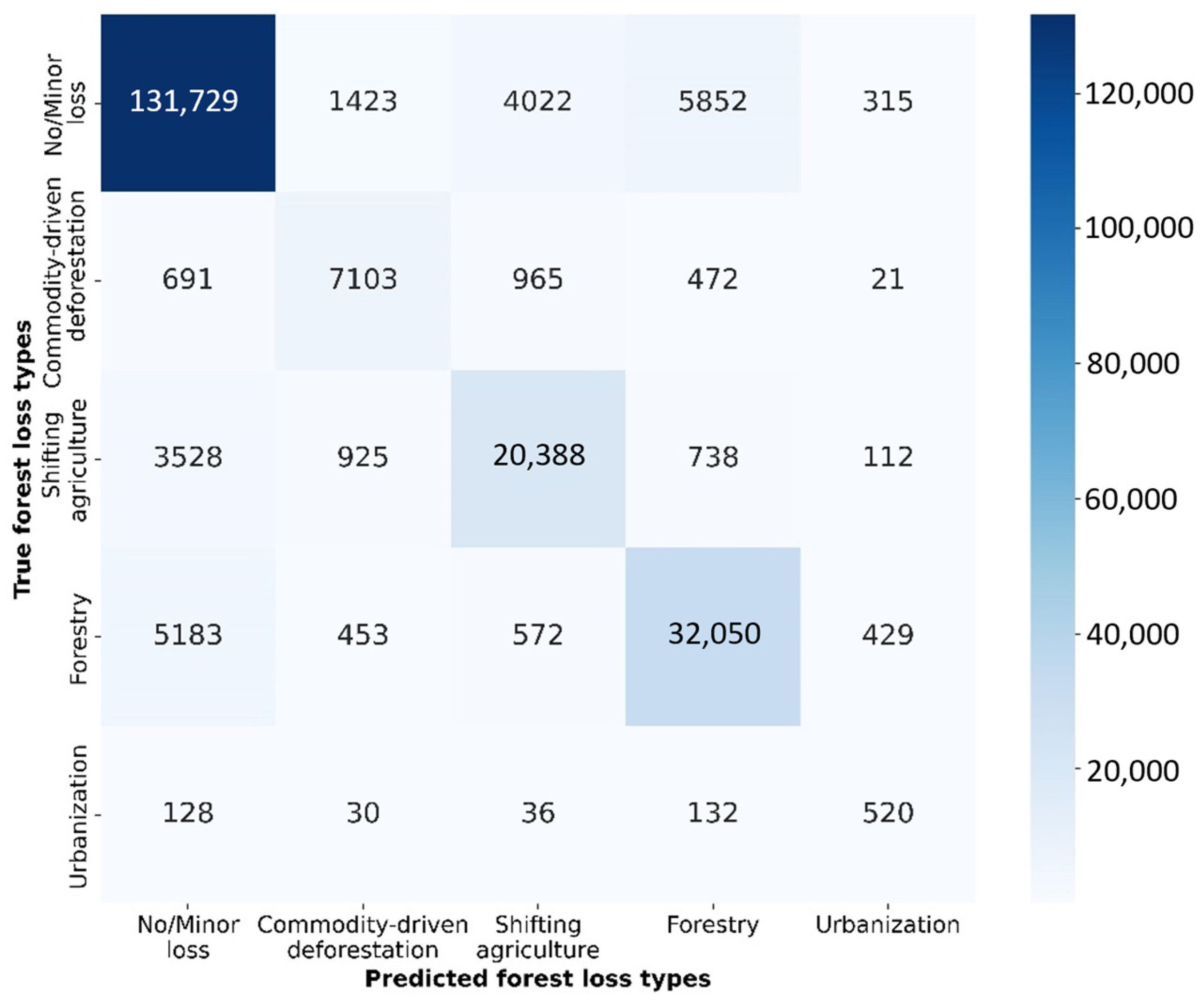
Figure 1. Study framework [10,23,28,29].
Remotesensing 15 03831 g001
Figure 2. Study area.
Remotesensing 15 03831 g002
Figure 3. The confusion matrix of the LightGBM classification model. The color shades of the squares indicate the number of samples. The numbers on the diagonal line of the confusion matrix indicate the numbers of correctly predicted samples.
Remotesensing 15 03831 g003
Figure 4. Cross-validation results of four forest loss area regression models. The color tone represents the sample size of the corresponding value. (a) commodity-driven deforestation (b) shifting agriculture (c) forestry (d) urbanization.
Remotesensing 15 03831 g004
Figure 5. Forest loss areas and the driving factors in China from 1900 to 2000.
Remotesensing 15 03831 g005
Figure 6. Spatial distribution patterns of forest loss in China from 1900 to 2000. Areas with significant forest loss driven by urbanization are shown in the zoomed-in windows.
Remotesensing 15 03831 g006
Figure 7. Comparison of forest loss from different data sources in China from 1900 to 2000.
Remotesensing 15 03831 g007
Figure 8. Comparison of the disturbance of forest loss from (ad) this study and (eh) HILDA+ datasets.
Remotesensing 15 03831 g008
Table 1. Summary of evaluation indices of the LightGBM classification model.
Forest Loss TypePrecisionRecallF1-ScoreNumber of SamplesAccuracy
No or minor loss0.920.930.93141,2590.88
Commodity driven deforestation0.770.720.749934
Shifting agriculture0.790.780.7925,983
Forestry0.830.820.8239,244
Urbanization0.610.370.461397
Macro average0.780.720.75217,817-
Weighted average0.880.880.88217,817-
Disclaimer/Publisher’s Note: The statements, opinions and data contained in all publications are solely those of the individual author(s) and contributor(s) and not of MDPI and/or the editor(s). MDPI and/or the editor(s) disclaim responsibility for any injury to people or property resulting from any ideas, methods, instructions or products referred to in the content.

