Synthesis of Synthetic Hyperspectral Images with Controllable Spectral Variability Using a Generative Adversarial Network

Abstract

In hyperspectral unmixing (HU), spectral variability in hyperspectral images (HSIs) is a major challenge which has received a lot of attention over the last few years. Here, we propose a method utilizing a generative adversarial network (GAN) for creating synthetic HSIs having a controllable degree of realistic spectral variability from existing HSIs with established ground truth abundance maps. Such synthetic images can be a valuable tool when developing HU methods that can deal with spectral variability. We use a variational autoencoder (VAE) to investigate how the variability in the synthesized images differs from the original images and perform blind unmixing experiments on the generated images to illustrate the effect of increasing the variability.

1. Introduction

Endmember variability poses a significant challenge for linear unmixing methods that use scale-invariant objective functions. The linear mixing model (LMM) models the spectrum of a pixel ${\mathit{x}}_p$ for an HSI $\mathit{Y}\in {\mathbb{R}}^{P\times B}$ having P pixels and B bands as a convex combination of the endmembers:

$${\mathit{x}}_p=\mathit{A}{\mathit{s}}_p+{ϵ}_p,\mathrm{subject}\mathrm{to}{\mathbf{1}}^T{\mathit{s}}_p=1\mathrm{and}{\mathit{s}}_p\ge \mathit{0},$$

(1)

where the abundance fractions ${\mathit{s}}_p$ are the area proportions of the endmembers in the pixel and ${ϵ}_p$ is the noise. The matrix $\mathit{A}$ is the endmember matrix, having the endmembers as its columns. When looking at Equation (1), we see that the LMM cannot model the spectral variability, which is a significant limitation. In remote sensing, the spectral variability is mainly caused by atmospheric effects, variation in illumination and topography, and intrinsic variations in the spectral signatures of the material itself [1]. Considerable effort has been put into developing HU techniques that handle spectral variability better.

Dealing with spectral variability has mainly been accomplished in two ways. One is using bundles of endmembers to represent each endmember class, with the bundles acquired from the data themselves or through field campaigns [2]. The other way is modeling the endmember variability using physical or statistical modeling. This requires extending the LMM in such a way that the endmembers can be different for each pixel. Some examples of such extended models are the augmented LMM [3], the extended LMM [4], and the perturbed LMM [5].

Numerous datasets exhibit two deficiencies when it comes to examining the impacts of spectral variability on methods. First, real datasets do not possess an easily quantifiable degree of spectral variability. Secondly, generated datasets typically have either zero spectral variability, or it is frequently produced based on a straightforward model, such as an augmented or extended linear mixing model [3,4], which makes the spectral variability somewhat rudimentary. It should be noted that there are advanced and complex methods, such as those in [6], that can be used to simulate HSIs with physical simulations using advanced radiometric and geometric models.

Recently, deep generative models have been employed in the generation of HSIs. By learning the distribution of actual images, they can generate new samples from the same distribution. One example is in [7], where a generative adversarial network (GAN) [8] was utilized to create realistic synthetic HSIs for data augmentation in hyperspectral classification tasks. Another significant type of deep generative model is the variational autoencoder (VAE) [9], which employs a different method to learn the data distribution and generate new samples.

VAEs are especially adept at modeling complex, high-dimensional data and continuous latent spaces, making them extremely useful for tasks like generating diverse sets of similar images. VAEs have been used for a wide range of applications, including image processing, data augmentation [10], image generation [11], game design [12], and hyperspectral unmixing. An instance of using a VAE for generating HSIs was demonstrated in [13], where a VAE was used to create synthetic HSIs with adjustable spectral variability. Diffusion models [14] present yet another distinct approach to data generation. The concept behind diffusion models is to portray the data generation process as a diffusion procedure that incrementally introduces noise to the original data over time, converting it into a simple distribution. To produce new data, the process is reversed; initiating from noise, the model applies a series of transformations that progressively eliminate the noise, resulting in a sample from the data distribution. These transformations are guided by a neural network, which is trained to predict how to denoise a data sample at each stage of the diffusion process.

This paper proposes a method to generate synthetic hyperspectral images using the linear mixing model (LMM) but with a controllable synthetic variability and ground truth for both the endmembers and abundance maps. The method employs a generative adversarial network (GAN), specifically a conditional Wasserstein GAN (WGAN) with a gradient penalty, that learns to generate new samples from the learned data distribution of a real hyperspectral image (HSI). The diversity or variability of the sampled endmembers can be efficiently tuned by two parameters.

The rest of this paper is organized as follows. Section 2.1 briefly introduces GANs. Section 2.2 describes the proposed method. Section 3 presents the results of the experiments, and finally, conclusions are drawn in Section 4.

2. Materials and Methods

2.1. Generative Adversarial Networks

GANs were first introduced in 2014 [8] as a generative model that can learn the distribution $P_r$ of the training data and generate new samples from the distribution. It consists of two neural networks, a generator G, and a discriminator D that are trained simultaneously. The generator G takes a latent code $\mathit{z}$ sampled from some prior distribution $p\left(\mathit{z}\right)$ as an input and outputs a generated sample $G\left(\mathit{z}\right)$. The discriminator D is trained to discriminate the generated samples from the real ones. G and D then compete with each other in a min-max game. The min-max objective of a GAN is

$$\begin{array}{cc}\hfill \underset{G}{\min }\underset{D}{\max }V(G,D)& ={\mathbb{E}}_{\mathit{x}\sim P_r}\left[\log D\left(\mathit{x}\right)\right]\hfill \\ \hfill & +{\mathbb{E}}_{\widehat{\mathit{x}}\sim P_g}\left[\log (1-D\left(\tilde{\mathit{x}}\right))\right],\hfill \end{array}$$

(2)

where $P_g$ is the model distribution, implicitly defined as $\tilde{\mathit{x}}=G\left(\mathit{z}\right),\mathit{z}\sim p\left(\mathit{z}\right)$, and p is the distribution of the latent codes. The generator tries to minimize this objective function, and the discriminator tries to maximize it.

This objective function is not ideal as the generator saturates during training and stops learning as it gets too little feedback from the discriminator. To help stabilize training and prevent mode collapse in the generator, the Wasserstein GAN [15] with a gradient penalty was developed (WGAN-GP). The objective function becomes

$$\begin{array}{cc}\hfill \underset{G}{\min }\underset{D\in \mathcal{F}}{\max }V(G,D)& =\underset{\mathit{x}\sim P_r}{\mathbb{E}}\left[D\left(\mathit{x}\right)\right]-\underset{\tilde{\mathit{x}}\sim P_g}{\mathbb{E}}\left[D\left(\tilde{\mathit{x}}\right)\right]\hfill \\ \hfill & +\lambda \underset{\widehat{\mathit{x}}\sim P_{\widehat{\mathit{x}}}}{\mathbb{E}}\left[\right(\parallel {\nabla }_{\widehat{\mathit{x}}}D\left(\widehat{\mathit{x}}\right){\parallel }_2-1{)}^2],\hfill \end{array}$$

(3)

where $\mathcal{F}$ is the set of 1-Lipschitz functions [16], $\widehat{\mathit{x}}$ is a convex combination of $\mathit{x}$ from the real distribution and $\tilde{\mathit{x}}$ from the model distribution, $\widehat{\mathit{x}}=ϵ\mathit{x}+(1-ϵ)\tilde{\mathit{x}}$, $ϵ$ is a number between 0 and 1, and $\lambda$ is the gradient penalty parameter. The gradient penalty softly enforces the critic (as the discriminator is called for WGANs) to be 1-Lipschitz, a necessary condition for the first two terms to be equivalent to the so-called Earth mover’s distance between the distributions. The critic outputs a nonnegative score instead of a probability.

2.2. The Proposed Method

The proposed method uses a conditional WGAN with gradient penalty and total variation [17] (TV) regularization on the output of the generator. The TV regularization is needed to smooth the noisy output of the generator. A conditional GAN enables conditional generation by labeling the inputs to both the generator and discriminator. Thus, the latent codes are a combination of a noise vector sampled from a truncated Gaussian distribution and a label vector.

Figure 1a shows a schematic of the proposed WGAN-GP-TV network. The pixels are labeled as Figure 1b illustrates. Since there were generally no class labels in the ground truth for the hyperspectral image used for training, we constructed them from the ground truth abundance maps for the image. Each pixel was labeled with a weighted one-hot vector, where the index of the one indicates the endmember class of the pixel as determined by which endmember has the greatest abundance fraction. The one-hot vector is then multiplied by the highest abundance which indicates the purity. The loss function used is

$$\begin{array}{cc}\hfill \mathcal{L}& ={\mathbb{E}}_{\tilde{\mathit{x}}\sim P_g,\mathit{y}\sim P_r\left(y\right)}\left[D(\tilde{\mathit{x}},\mathit{y})\right]-{\mathbb{E}}_{\mathit{x},\mathit{y}\sim P_r}\left[D(\mathit{x},\mathit{y})\right]\hfill \\ \hfill & +\lambda {\mathbb{E}}_{\widehat{\mathit{x}}\sim P_{\widehat{\mathit{x}}},\mathit{y}\sim P_r\left(\mathit{y}\right)}\left[(\parallel {\nabla }_{\widehat{\mathit{x}}}D(\widehat{\mathit{x}},\mathit{y}){{\parallel }_2-1)}^2\right]\hfill \\ \hfill & +{\lambda }_{\mathrm{TV}}\mathrm{TV}\left(\tilde{\mathit{x}}\right).\hfill \end{array}$$

(4)

Here, $\mathit{y}$ represents the labels we are conditioning on, $\widehat{\mathit{x}}$ is an interpolation between the fake and real samples, ${\lambda }_{\mathrm{TV}}$ is the total variation penalty parameter, and $\mathrm{TV}\left(\tilde{\mathit{x}}\right)$ is the total variation of the generator’s output. It should be noted that the 2-norm of the gradient is generally used for the gradient penalty in the literature. Weight clipping can also be used to enforce the critic to be 1-Lipschitz, but this has been found to be unstable [15]. By conditioning both G and D on the labels, $\mathit{y}$, the generator can generate specific endmembers with varying purity.

To control the variability of the sampled endmembers, we employed the truncation trick [18], a latent sampling procedure where we sampled the codes $\mathit{z}$ from a truncated normal distribution. High truncation values correspond to a broad distribution, and low values correspond to a narrow distribution. Truncation trades fidelity for diversity. If we sample from a narrow distribution, then the variability of the sampled endmembers from the generator will be small, and vice versa. This can be interpreted as the extent to which the learned variability in the training data is used to generate new samples.

We constructed the synthetic HSIs by sampling a set of endmembers ${\mathit{A}}_p$ for every pixel ${\mathit{x}}_p$ having ground truth abundances ${\mathit{s}}_p$ and constructing the synthetic pixels as

$${\mathit{x}}_p={\mathit{A}}_p{\mathit{s}}_p.$$

(5)

The spectral variability is controlled by the truncation value and by specifying a minimum purity value. When sampling latent codes from the truncated normal, the purity is sampled uniformly between the minimum purity and 1.0. The ground truth endmembers for the synthetic HSI are obtained as the average of a large number of sampled endmembers.

3. Experiments and Results

3.1. Experimental Set-Up

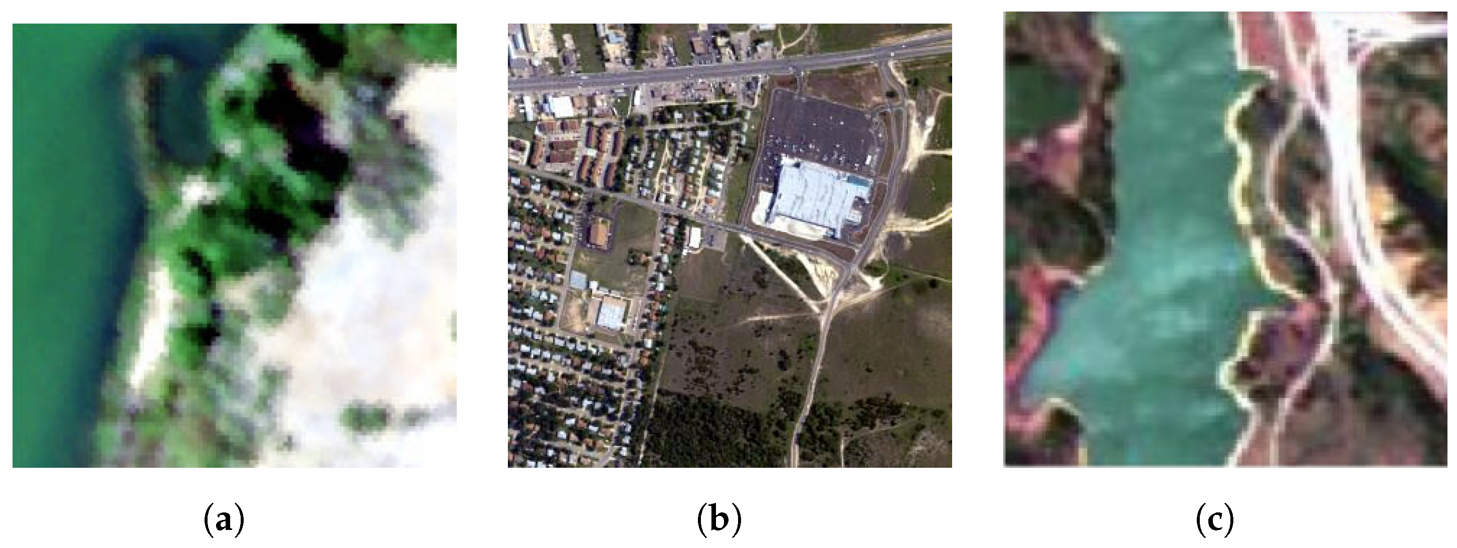
We trained the GAN on the widely used Urban, Samson, and Jasper datasets. The Urban HSI is 307 by 307 pixels and has 162 usable bands covering the 400–2500 nm wavelength range. We used the ground truth abundances for four reference endmembers. The Jasper HSI is 100 by 100 pixels with 198 usable bands and has 4 endmembers. The Samson HSI is 95 by 95 pixels, and the number of bands is 145, covering the 401–889 nm wavelength range. The dataset has the following endmembers: Water, Soil, and Tree. Figure 2 shows the simulated RGB images of the datasets.

The GAN was trained for 300 epochs using the Adam optimizer for both the generator and critic. The critic was trained for five iterations for every iteration of the generator. The learning rate was set to 0.0002, the gradient penalty $\lambda$ was set to 10.0, and the TV penalty ${\lambda }_{\mathrm{TV}}$ was set to $0.00003$. The latent dimension of the sampled noise was set to 10.

3.2. Evaluation

In order to investigate and compare the spectral variability of the original and synthetic images, we utilized a variational autoencoder. Specifically, the $\beta$-VAE model, as referred to in [19], was employed. The encoder of the VAE was used to generate images that illustrated the distributions of the encoding in a two-dimensional latent space.

Subsequently, we performed blind unmixing on the Urban synthetic datasets which demonstrated varying spectral variability. This was achieved using two distinct methods. The first method employed an autoencoder-based CNNAEU as per [20], while the second involved a sparsity-constrained nonnegative matrix factorization termed ${\mathsf{\ell }}_{1/2}$-NMF, as referenced in [21]. The ${\mathsf{\ell }}_{1/2}$-NMF method separates the given HSI into two matrices: one of abundances and another of endmembers. This method was founded on the ${\mathsf{\ell }}_{1/2}$-norm, a convex relaxation of the ${\mathsf{\ell }}_0$-norm. The first method has been proven to be more robust against spectral variability as it incorporates the spectral-angle-distance (SAD) objective function, unlike the NMF method, which utilizes the MSE objective function. The NMF method is a traditional approach frequently used for unmixing and is appropriate for HSIs exhibiting low spectral variability.

We then compared our method with synthetic datasets constructed using both the linear mixing model (LMM) and the Hapke model as cited in [22] in order to introduce variability. The Hapke model is employed to simulate variability resulting from variations in topography. In this instance, we utilized it to generate several variants of reference endmembers that corresponded to different observation angles, assuming a Lambertian approximation.

To assess the performance of the unmixing methods, we employed the mean SAD between the estimated and ground truth endmembers:

$$\mathrm{mSAD}=\frac{1}{R}\sum _{i=1}^R\arccos \left(\frac{\langle {\widehat{\mathit{m}}}_i,{\mathit{m}}_i\rangle }{{∥{\widehat{\mathit{m}}}_i∥}_2{∥{\mathit{m}}_i∥}_2}\right),$$

(6)

where R is the number of endmembers, ${\widehat{\mathit{m}}}_i$ represents the endmembers extracted by the method, and ${\mathit{m}}_i$ represents the reference endmembers. The lower the mSAD, the higher the similarity.

3.3. Results and Analysis

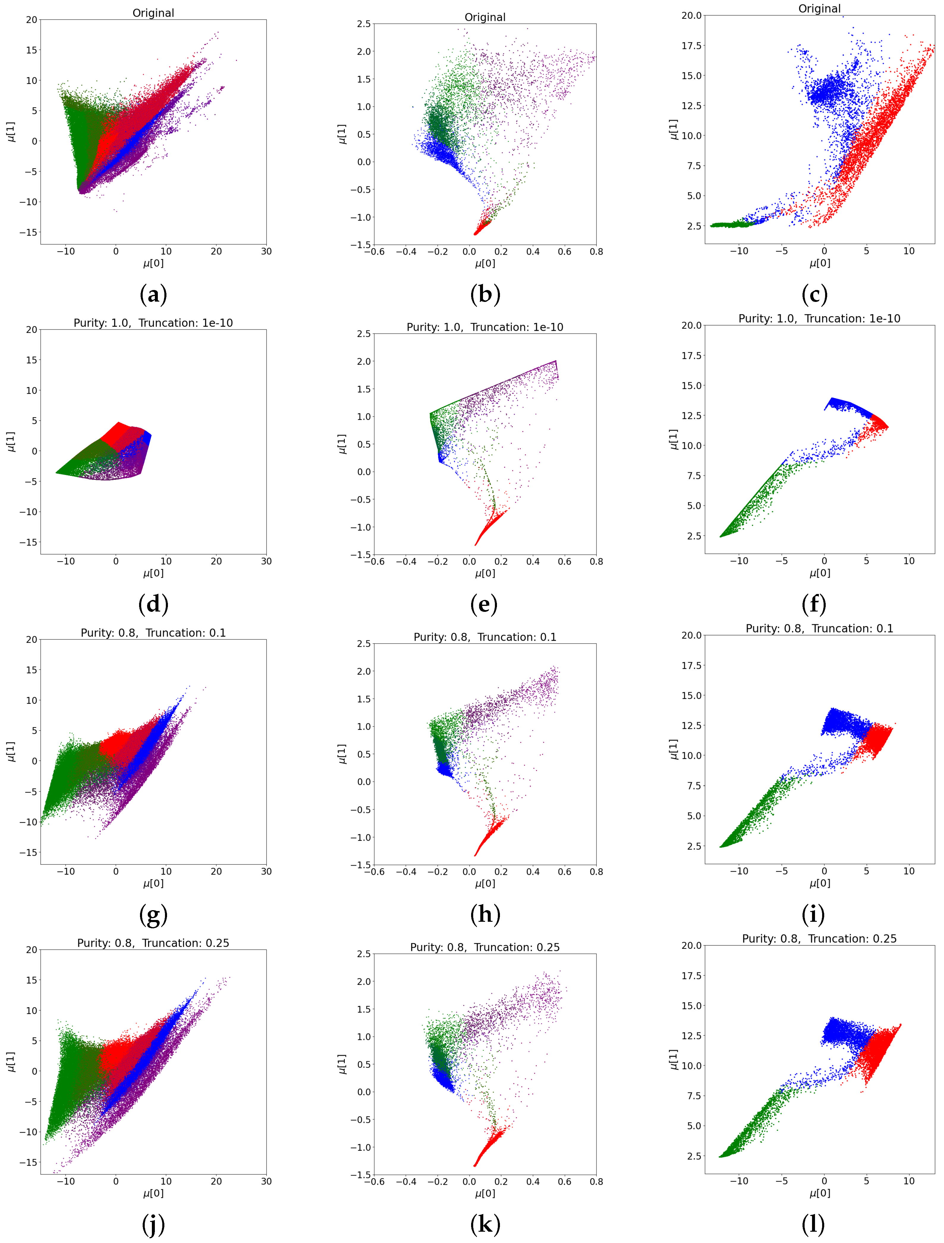
Figure 3 displays the original images, along with three synthetic images for each HSI with increasing spectral variability, in the VAE’s latent space. Figure 3d–f exhibit zero spectral variability, with fixed endmembers for every pixel (i.e., LMM reconstruction of the original image). As can be seen from Figure 3, the spectral variability for the high truncation values was akin to that in the original images, despite the simplified construction according to Equation (5).

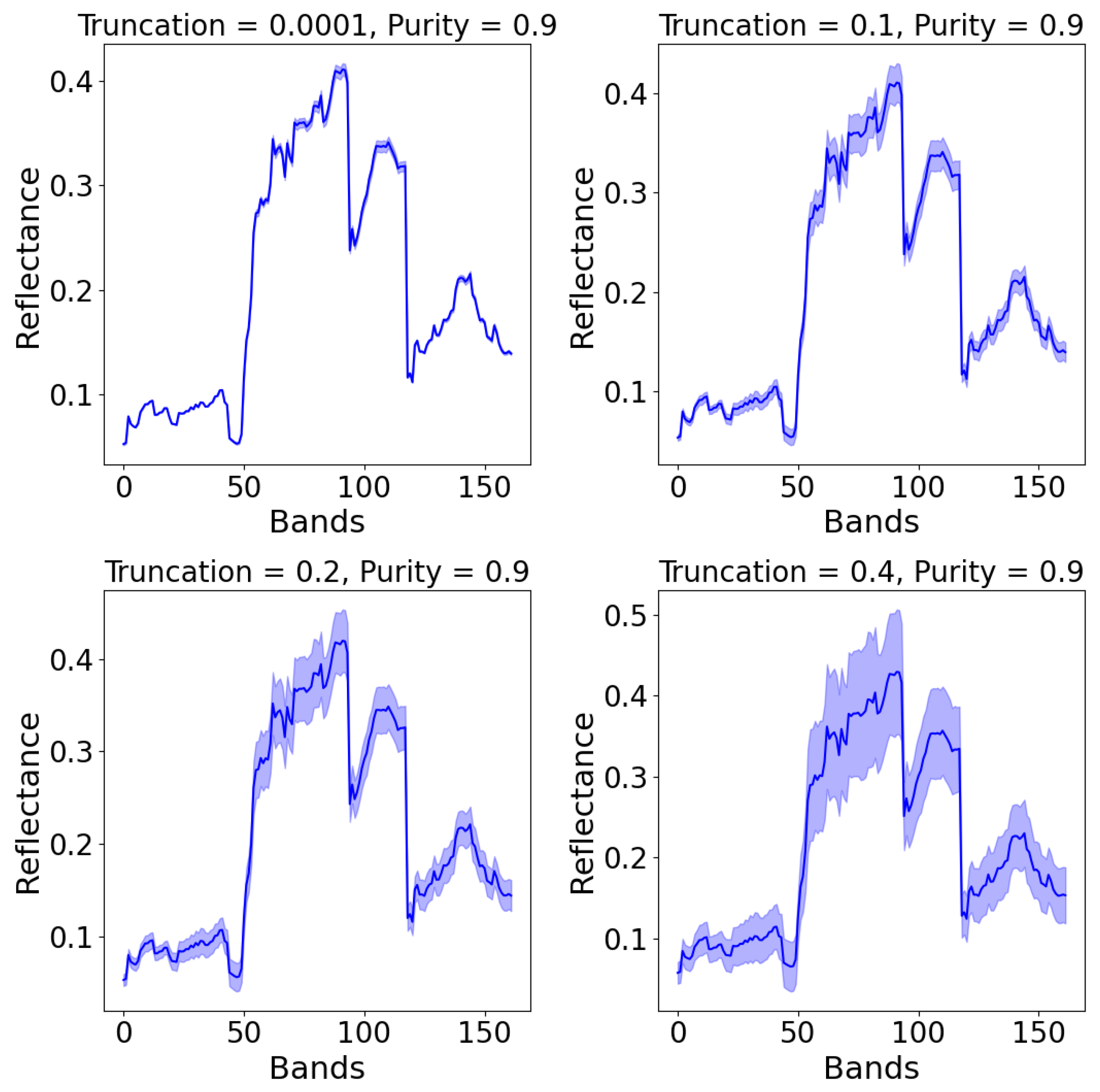
Figure 4 demonstrates the effect of different truncation values on the grass endmember of the Urban dataset. The solid line represents the average, while the shaded region indicates the standard deviation. The plot used 150 samples from the GAN’s generator. It clearly shows that the variability increased with an increasing truncation value.

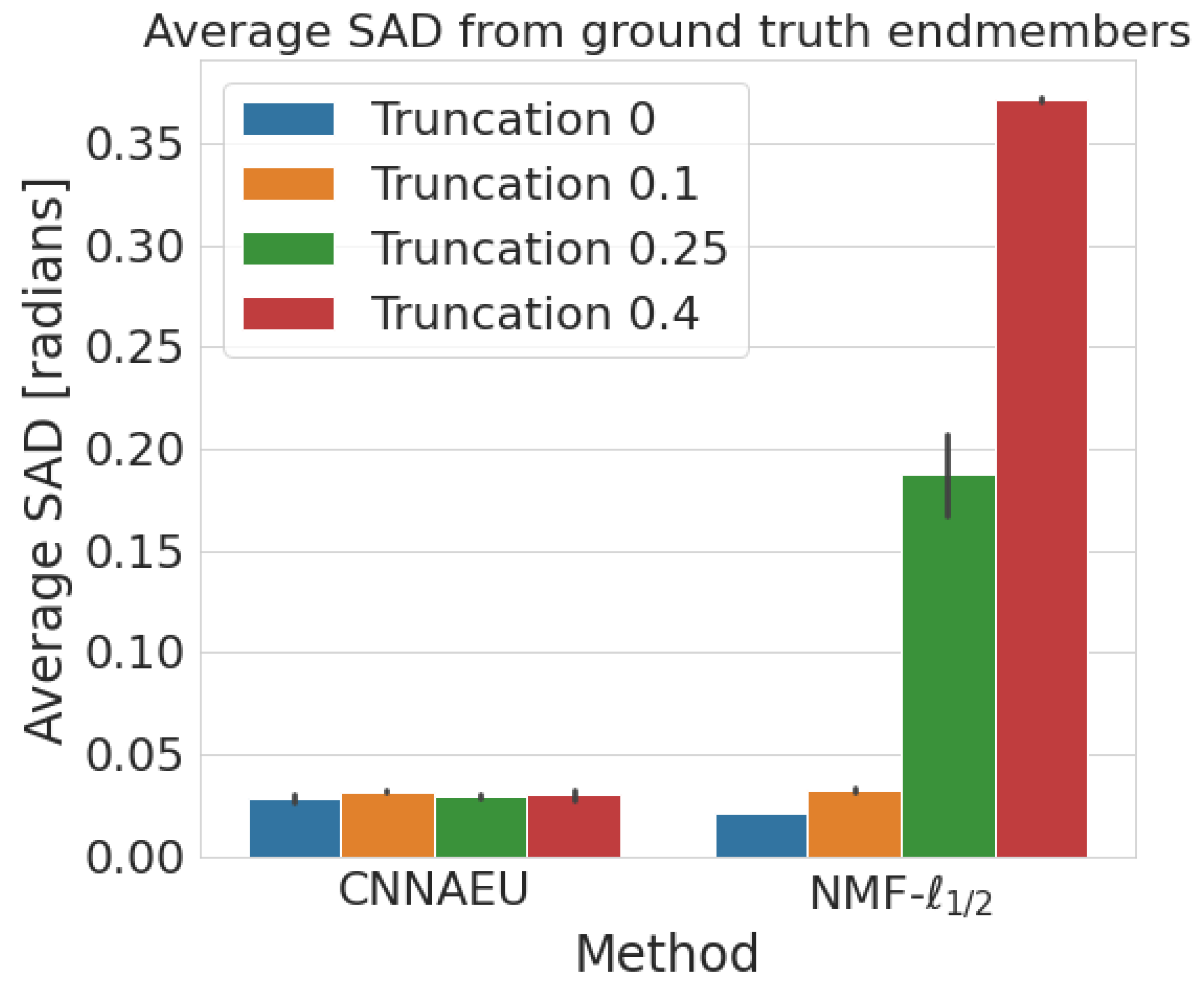
We performed blind unmixing on the synthetic Urban images displayed in the left column of Figure 3 and additionally on an image with a truncation of 0.4 and purity of 0.75. Figure 5 presents the results of the experiment in terms of the average SAD in radians from the ground truth endmembers. Each experiment comprised 10 runs. Figure 5 illustrates that the method using a scale-invariant objective function (CNNAEU) encountered no difficulties with increasing spectral variability, whereas the traditional method employing MSE exhibited progressively poorer performance. The ${\mathsf{\ell }}_{1/2}$-NMF method recorded the lowest SAD for zero spectral variability. This fact, along with the low SAD values, suggests that the ground truth endmembers were a reliable ground truth for the synthetic images.

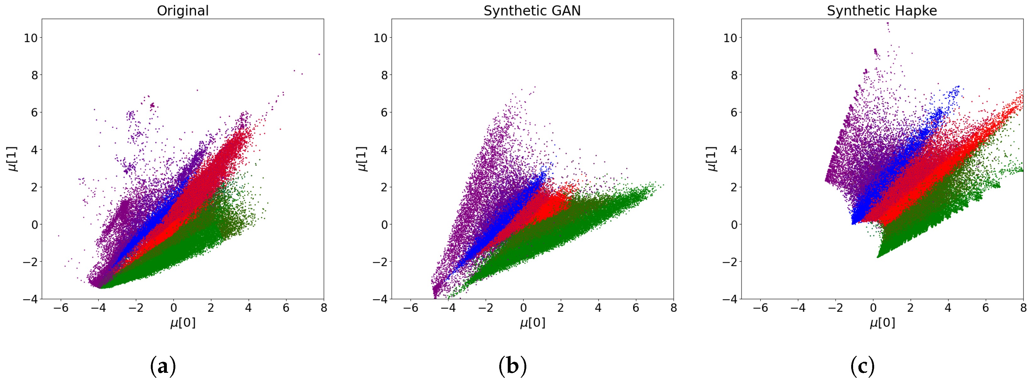
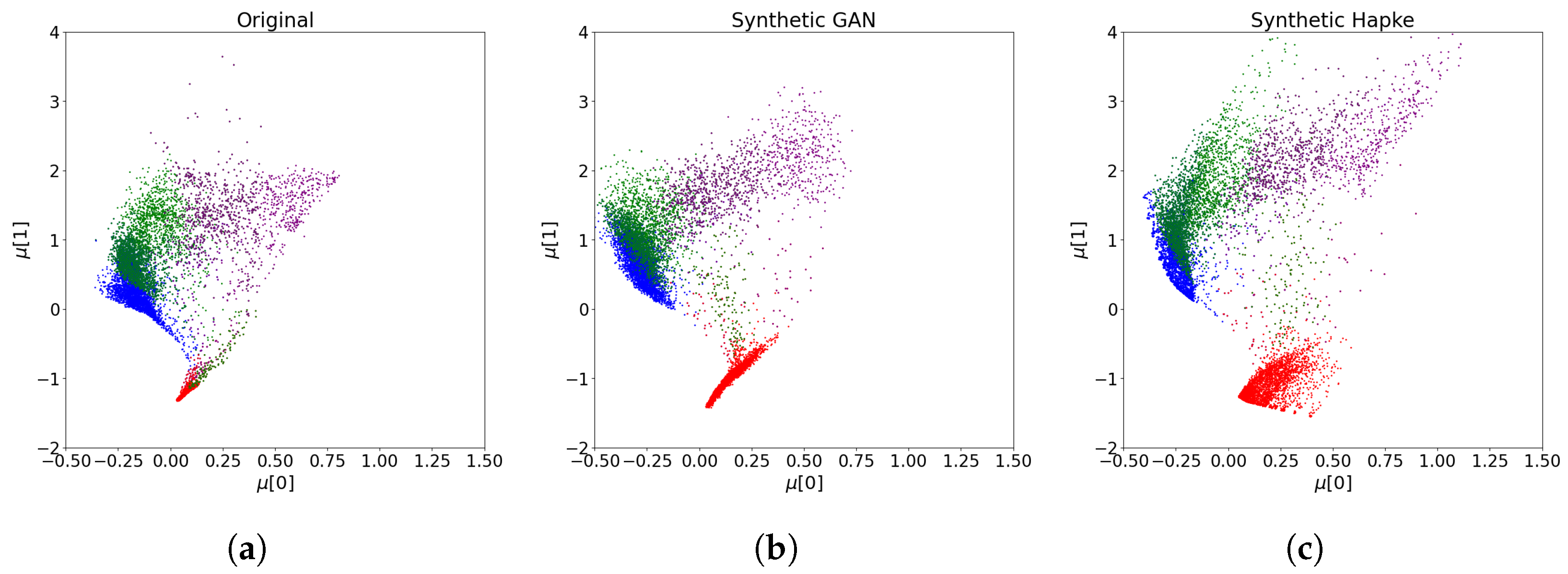
Figure 6 shows the latent codes for the original Urban dataset, a synthetic version created using the proposed method, and a synthetic version constructed using the Hapke model. As can be seen from Figure 6, the Hapke model did not capture the variability as well as the proposed method, suggesting that factors other than topography, such as natural biological variability in vegetation, were at work. Figure 7 shows the same encodings but for the Jasper dataset. Again, it can be seen that the Hapke model did not capture the variability as well as the proposed method. It should be noted that the latent code projection in these two figures is slightly different from that of Figure 3.

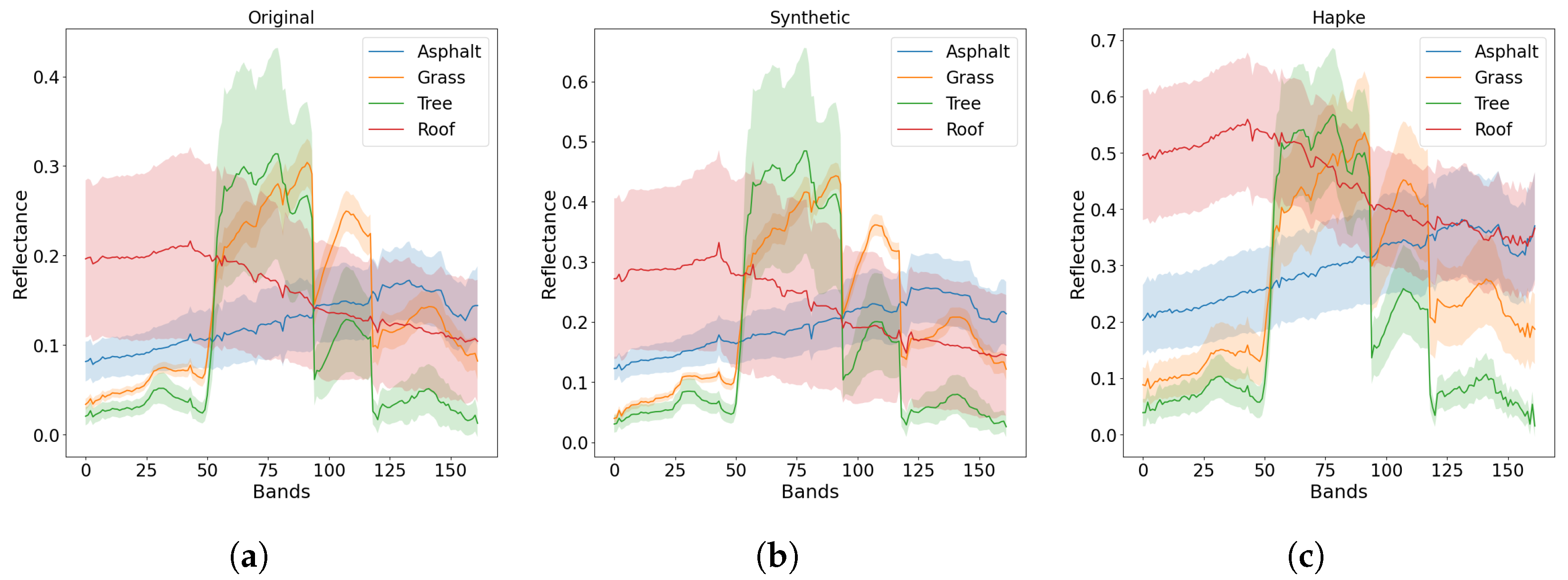
We could further evaluate the method by comparing the mean and variance of the mostly pure pixels in the original and synthetic images. Figure 8 shows the average of mostly pure pixels (with the largest fractional abundance >0.8) for the original Urban HSI, the synthetic HSI with a truncation of 0.4 and purity of 0.75, and the Hapke synthetic HSI. As can be seen from the figure, the mean spectra for the original and GAN-simulated images were very similar in relative shape and scale and had incredibly similar variances (shaded areas). However, the magnitude of the mean spectra was higher for the image simulated using the proposed method. This was most likely a result of the LMM construction of the synthetic image. The mean spectra for the synthetic image generated using the Hapke model was not all that similar to the mean spectra for the original image.

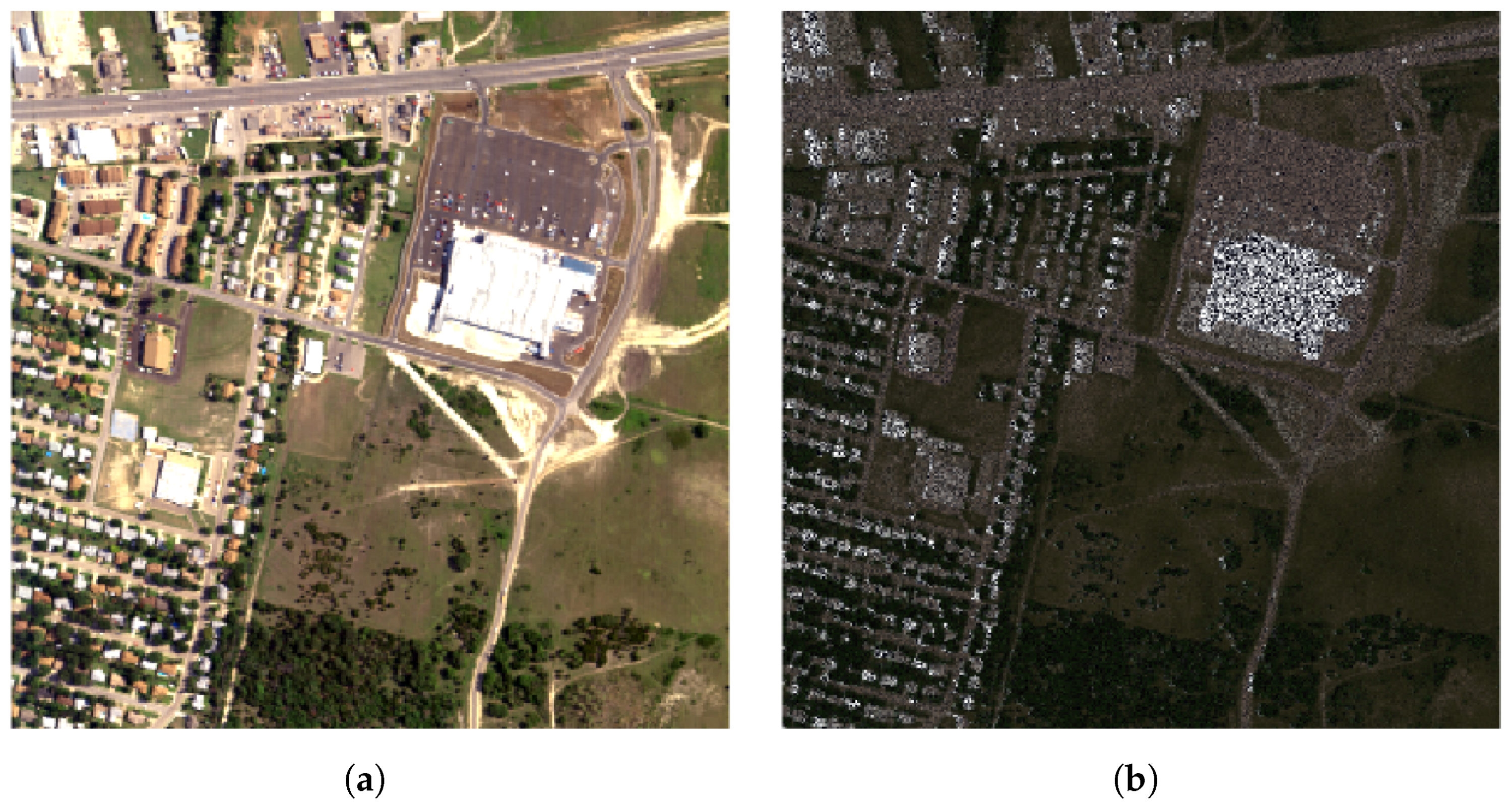
Figure 9 shows simulated RGB images of the original Urban dataset and the synthetic images with a truncation of 0.4 and purity of 0.75. It is clear from the figure that there is a substantial difference between the original and synthetic images. The synthetic images appear to be much dimmer and flatter than the original image and also appear to be noisy. This is due to the simplistic LMM construction of the synthetic images and because the method is not spatial in nature (i.e., endmembers are randomly sampled for each pixel).

4. Conclusions

In this paper, we proposed a technique that generates synthetic datasets that have a controllable degree of variability while having the ground truths for both the abundances and endmembers. The variability is generated by a conditional Wasserstein GAN that has learned the distribution of the original real image. The spectral variability is controlled by two parameters, the truncation of the prior normal distribution and the purity. Experiments showed that the generated spectral variability approximated the original one. Blind unmixing experiments showed that the ground truth reference endmembers were a good ground truth for the synthetic images and illustrated the effects of increasing variability on the performance of the methods.

References

1. Borsoi, R.; Imbiriba, T.; Bermudez, J.C.; Richard, C.; Chanussot, J.; Drumetz, L.; Tourneret, J.Y.; Zare, A.; Jutten, C. Spectral Variability in Hyperspectral Data Unmixing: A Comprehensive Review. IEEE Geosci. Remote Sens. Mag. 2021, 9, 223–270. [Google Scholar] [CrossRef]
2. Uezato, T.; Fauvel, M.; Dobigeon, N. Hyperspectral Unmixing with Spectral Variability Using Adaptive Bundles and Double Sparsity. IEEE Trans. Geosci. Remote Sens. 2019, 57, 3980–3992. [Google Scholar] [CrossRef] [Green Version]
3. Hong, D.; Yokoya, N.; Chanussot, J.; Zhu, X.X. An Augmented Linear Mixing Model to Address Spectral Variability for Hyperspectral Unmixing. IEEE Trans. Image Process. 2019, 28, 1923–1938. [Google Scholar] [CrossRef] [PubMed] [Green Version]
4. Drumetz, L.; Veganzones, M.; Henrot, S.; Phlypo, R.; Chanussot, J.; Jutten, C. Blind Hyperspectral Unmixing Using an Extended Linear Mixing Model to Address Spectral Variability. IEEE Trans. Image Process. 2016, 25, 3890–3905. [Google Scholar] [CrossRef] [PubMed] [Green Version]
5. Thouvenin, P.A.; Dobigeon, N.; Tourneret, J.Y. Hyperspectral Unmixing with Spectral Variability Using a Perturbed Linear Mixing Model. IEEE Trans. Signal Process. 2016, 64, 525–538. [Google Scholar] [CrossRef] [Green Version]
6. Zhao, H.; Jiang, C.; Jia, G.; Tao, D. Simulation of hyperspectral radiance images with quantification of adjacency effects over rugged scenes. Meas. Sci. Technol. 2013, 24, 125405. [Google Scholar] [CrossRef]
7. Liu, W.; You, J.; Lee, J. HSIGAN: A Conditional Hyperspectral Image Synthesis Method with Auxiliary Classifier. IEEE J. Sel. Top. Appl. Earth Obs. Remote Sens. 2021, 14, 3330–3344. [Google Scholar] [CrossRef]
8. Goodfellow, I.J.; Pouget-Abadie, J.; Mirza, M.; Xu, B.; Warde-Farley, D.; Ozair, S.; Courville, A.; Bengio, Y. Generative Adversarial Nets. In Proceedings of the 27th International Conference on Neural Information Processing Systems, Cambridge, MA, USA, 8–13 December 2014; Volume 2, pp. 2672–2680. [Google Scholar]
9. Kingma, D.P.; Welling, M. Auto-Encoding Variational Bayes. Stat 2014, 1050, 10. [Google Scholar]
10. Elbattah, M.; Loughnane, C.; Guérin, J.L.; Carette, R.; Cilia, F.; Dequen, G. Variational Autoencoder for Image-Based Augmentation of Eye-Tracking Data. J. Imaging 2021, 7, 83. [Google Scholar] [CrossRef]
11. Peng, J.; Liu, D.; Xu, S.; Li, H. Generating Diverse Structure for Image Inpainting With Hierarchical VQ-VAE. In Proceedings of the 2021 IEEE/CVF Conference on Computer Vision and Pattern Recognition (CVPR), Nashville, TN, USA, 19–25 June 2021; pp. 10770–10779. [Google Scholar] [CrossRef]
12. Mak, H.W.L.; Han, R.; Yin, H.H.F. Application of Variational AutoEncoder (VAE) Model and Image Processing Approaches in Game Design. Sensors 2023, 23, 3457. [Google Scholar] [CrossRef] [PubMed]
13. Palsson, B.; Ulfarsson, M.O.; Sveinsson, J.R. Synthetic Hyperspectral Images With Controllable Spectral Variability and Ground Truth. IEEE Geosci. Remote Sens. Lett. 2022, 19, 1–5. [Google Scholar] [CrossRef]
14. Dhariwal, P.; Nichol, A. Diffusion models beat gans on image synthesis. Adv. Neural Inf. Process. Syst. 2021, 34, 8780–8794. [Google Scholar]
15. Arjovsky, M.; Chintala, S.; Bottou, L. Wasserstein generative adversarial networks. In Proceedings of the International Conference on Machine Learning, PMLR, Sydney, Australia, 6–11 August 2017; pp. 214–223. [Google Scholar]
16. Cobzaş, Ş.; Miculescu, R.; Nicolae, A. Lipschitz Functions; Springer: Berlin/Heidelberg, Germany, 2019; Volume 2241. [Google Scholar]
17. Rudin, L.I.; Osher, S.; Fatemi, E. Nonlinear total variation based noise removal algorithms. Phys. D Nonlinear Phenom. 1992, 60, 259–268. [Google Scholar] [CrossRef]
18. Brock, A.; Donahue, J.; Simonyan, K. Large scale GAN training for high fidelity natural image synthesis. arXiv 2018, arXiv:1809.11096. [Google Scholar]
19. Higgins, I.; Matthey, L.; Pal, A.; Burgess, C.P.; Glorot, X.; Botvinick, M.M.; Mohamed, S.; Lerchner, A. beta-VAE: Learning Basic Visual Concepts with a Constrained Variational Framework. In Proceedings of the ICLR, 5th International Conference on Learning Representations, Toulon, France, 24–26 April 2017. [Google Scholar]
20. Palsson, B.; Ulfarsson, M.O.; Sveinsson, J.R. Convolutional Autoencoder for Spectral–Spatial Hyperspectral Unmixing. IEEE Trans. Geosci. Remote Sens. 2021, 59, 535–549. [Google Scholar] [CrossRef]
21. Qian, Y.; Jia, S.; Zhou, J.; Robles-Kelly, A. Hyperspectral Unmixing via L1/2 Sparsity-Constrained Nonnegative Matrix Factorization. IEEE Trans. Geosci. Remote Sens. 2011, 49, 4282–4297. [Google Scholar] [CrossRef] [Green Version]
22. Hapke, B. Bidirectional reflectance spectroscopy: 1. Theory. J. Geophys. Res. Solid Earth 1981, 86, 3039–3054. [Google Scholar] [CrossRef] [Green Version]
23. Magnusson, M.; Sigurdsson, J.; Armansson, S.E.; Ulfarsson, M.O.; Deborah, H.; Sveinsson, J.R. Creating RGB Images from Hyperspectral Images Using a Color Matching Function. In Proceedings of the IGARSS 2020—2020 IEEE International Geoscience and Remote Sensing Symposium, Waikoloa, HI, USA, 26 September–2 October 2020; pp. 2045–2048. [Google Scholar] [CrossRef]
Figure 1. Schematics of the proposed conditional WGAN (a) and how the pixels are labeled (b). Both the generator and the critic are conditioned on the labels which indicate the class and purity of every pixel. (a) Schematic of the conditional WGAN-GP-TV. (b) The labeling of a pixel having an abundance vector s p . The vector y p is the label.
Remotesensing 15 03919 g001
Figure 2. Simulated and actual RGB images of the datasets used in the experiments. (a) Samson (simulated); (b) Urban (simulated); and (c) Apex (actual).
Remotesensing 15 03919 g002
Figure 3. The latent space encodings of the original and synthetic images. The left column has the Urban images, and the right column has the Jasper images. Different colors indicate which endmember has the largest abundance fraction. The truncation and purity values are indicated in the titles and control the spectral variability of the synthetic images. (a) Original Urban HSI. (b) Original Jasper HSI. (c) Original Samson HSI. (d) Urban with zero variability. (e) Jasper with zero variability. (f) Samson with zero variability. (g) Urban with truncation value of 0.1 and purity of 0.8. (h) Jasper with truncation value of 0.1 and purity of 0.8. (i) Samson with truncation value of 0.1 and purity of 0.8. (j) Urban with truncation value of 0.1 and purity of 0.9. (k) Jasper with truncation value of 0.1 and purity of 0.9. (l) Samson with truncation value of 0.1 and purity of 0.9.
Remotesensing 15 03919 g003
Figure 4. The figure shows the effect of increasing truncation on the grass endmember of the Urban dataset. The solid line is the average, and the shaded region indicates the standard deviation. The plot uses 150 samples from the generator of the GAN.
Remotesensing 15 03919 g004
Figure 5. The average SAD from the ground truth endmembers for the original and three synthetic datasets with increasing spectral variability.
Remotesensing 15 03919 g005
Figure 6. Latent space encodings of the original Urban image, the GAN simulated synthetic image using a truncation of 0.5 and purity of 0.8, and the Hapke model’s simulated synthetic image. (a) The original Urban image. (b) Image with GAN (truncation of 0.5 and purity of 0.8); and (c) using the Hapke model.
Remotesensing 15 03919 g006
Figure 7. Latent space encodings of the original Jasper image, the GAN simulated synthetic image using a truncation of 0.5 and purity of 0.8, and the simulated image using the Hapke model. (a) The original Jasper image. (b) GAN with truncation of 0.5 and purity of 0.8. (c) Using the Hapke model.
Remotesensing 15 03919 g007
Figure 8. Average spectra of less mixed pixels (purity = 0.8) from the original Urban image, the GAN simulated synthetic image using a truncation of 0.4 and purity of 0.8, and the Hapke model’s simulated synthetic image. (a) The original Urban image. (b) GAN with truncation of 0.4 and purity of 0.8. (c) Using the Hapke model.
Remotesensing 15 03919 g008
Figure 9. Simulated RGB images of the original Urban HSI and an HSI created using the proposed method. The method in [23] was used to create the images. (a) The original Urban image. (b) GAN with truncation of 0.4 and purity of 0.8.
Remotesensing 15 03919 g009
Disclaimer/Publisher’s Note: The statements, opinions and data contained in all publications are solely those of the individual author(s) and contributor(s) and not of MDPI and/or the editor(s). MDPI and/or the editor(s) disclaim responsibility for any injury to people or property resulting from any ideas, methods, instructions or products referred to in the content.