Article

Joint Direction of Arrival-Polarization Parameter Tracking Algorithm Based on Multi-Target Multi-Bernoulli Filter

School of Automation (School of Artificial Intelligence), Hangzhou Dianzi University, Hangzhou 310018, China
*
Author to whom correspondence should be addressed.
Remote Sens. 2023, 15(16), 3929; https://doi.org/10.3390/rs15163929
Submission received: 12 July 2023 / Revised: 5 August 2023 / Accepted: 7 August 2023 / Published: 8 August 2023
(This article belongs to the Special Issue Advances in Radar Systems for Target Detection and Tracking)

Abstract

:
This paper presents a tracking algorithm for joint estimation of direction of arrival (DOA) and polarization parameters, which exhibit dynamic behavior due to the movement of signal source carriers. The proposed algorithm addresses the challenge of real-time estimation in multi-target scenarios with an unknown number. This algorithm is built upon the Multi-target Multi-Bernoulli (MeMBer) filter algorithm, which makes use of a sensor array called Circular Orthogonal Double-Dipole (CODD). The algorithm begins by constructing a Minimum Description Length (MDL) principle, taking advantage of the characteristics of the polarization-sensitive array. This allows for adaptive estimation of the number of signal sources and facilitates the separation of the noise subspace. Subsequently, the joint parameter Multiple Signal Classification (MUSIC) spatial spectrum function is employed as the pseudo-likelihood function, overcoming the limitations imposed by unknown prior information constraints. To approximate the posterior distribution of MeMBer filters, Sequential Monte Carlo (SMC) method is utilized. The simulation results demonstrate that the proposed algorithm achieves excellent tracking accuracy in joint DOA-polarization parameter estimation, whether in scenarios with known or unknown numbers of signal sources. Moreover, the algorithm demonstrates robust tracking convergence even under low Signal-to-Noise Ratio (SNR) conditions.

Graphical Abstract

1. Introduction

In the fields of sonar, radar and remote sensing, direction of arrival (DOA) estimation has been a prominent and extensively researched area for many years. It plays a crucial role in various applications, such as target detection, tracking and classification. Several high-resolution DOA estimation algorithms have been developed over the past few decades, including Multiple Signal Classification (MUSIC) [1,2,3,4], Estimation of Signal Parameters via Rotational Invariance Techniques (ESPRIT) [5] and subspace fitting [6,7,8], among others. Furthermore, DOA estimation has branched out into two important areas: DOA tracking and joint DOA-polarization parameter estimation based on polarization-sensitive arrays.
In terms of DOA tracking, effective approaches have been developed to address the challenges of computational complexity and performance degradation caused by spatial-temporal spectrum expansion resulting from the movement of signal source carriers. Yang et al. [9] proposed Projection Approximation Subspace Tracking (PAST) and PAST with deflation (PASTd) algorithms to update subspaces in real time based on an unconstrained minimization problem. Orton et al. [10] utilized the particle filter algorithm for DOA tracking by incorporating prior information about the signal and noise. The Sequential Monte Carlo (SMC) method is employed in this algorithm to achieve accurate tracking. However, the aforementioned algorithms only consider a fixed number of DOA signals and cannot handle scenarios with time-varying DOA signal numbers. To address this limitation, Mahler et al. [11,12,13] introduced the concept of Random Finite Sets (RFS), where the state and measurement of multiple targets are modeled as RFS, and RFS filtering algorithms are constructed within the Bayesian framework. This provides a novel approach to tracking the number of targets, especially in scenarios with time-varying variations. Notable RFS filters include Probability Hypothesis Density (PHD), Cardinalized PHD (CPHD) and multi-Bernoulli filters. Nannuru et al. [14] proposed an approximation method for PHD and CPHD filters specifically designed for the intensity superposition model under Gaussian noise conditions. Saucan et al. [15] introduced an approximate CPHD filter DOA tracking algorithm for multi-element extended targets in the presence of pulse noise. Choppala et al. [16] employ the MUSIC spectral function as the pseudo-likelihood function for Multi-Target Multi-Bernoulli (MeMBer) filter, enabling DOA tracking. Wu et al. [17] utilized a MeMBer tracking algorithm based on spatial smoothing to track DOA parameters using single snapshot measurements. Zhao et al. [18,19] utilized the Generalized Labeled Multi-Bernoulli (GLMB) filter to track DOA parameters.
Joint parameter estimation for DOA and polarization benefits from the advancement made in polarization-sensitive arrays. These arrays enable the system to capture the complete polarization domain information of the signal, leading to enhanced performance in multidimensional parameter estimation compared to traditional arrays. Classical signal parameter estimation methods, such as the MUSIC algorithm and ESPRIT, have been adapted for polarimetric-sensitive arrays to achieve a joint estimation of spatial-polarization domain parameters [20,21,22,23,24,25,26,27,28,29]. Additionally, the polynomial rooting method has been utilized with polarization-sensitive arrays to alleviate the computational burden associated with multidimensional parameter searches [30,31,32]. Qiu et al. [33] proposed a maximum-likelihood method for joint DOA and polarization estimation using manifold separation-oriented vector modeling technology. Chalise et al. [34] presented a sparse array composed of dual-polarized antenna elements and introduced a Compressed Sensing (CS) approach for joint estimation of DOA and polarization parameters. Shao et al. [35] addressed the problem of estimating the DOA of polarization signals by employing sparse vector matrices based on Maximum Array Spacing Constraint (MISC). Wang et al. [36] addressed the issue of signal covariance matrix rank deficiency caused by coherent signal sources using the oblique projection algorithm. Yue et al. [37] proposed a closed-form two-dimensional DOA and polarization joint estimation method based on a sparse multi-polarized antenna array. Furthermore, He et al. [38] proposed a DOA and polarization estimation algorithm based on dimensionality reduction MUSIC to overcome the high-dimensional search problem commonly encountered in multidimensional MUSIC methods.
In the context of electronic countermeasures, the utilization of polarization information in signal sources plays a crucial role in enhancing the anti-jamming capability and target detection performance of radar systems. To fully exploit and utilize polarization information, the tracking of joint DOA-polarization parameters has become increasingly important. However, there is limited research available on joint DOA-polarization parameter tracking. Traditional subspace tracking algorithms are not well-suited for this purpose, and particle filters exhibit significant performance degradation when tracking multidimensional parameters and are unable to handle the time-varying number of signal sources.
Based on the aforementioned analysis, this study proposes a DOA-polarization joint parameter tracking particle filter based on the MeMBer filter. The main innovations of this research are as follows:
  • Investigation of joint DOA-polarization parameter estimation based on a uniform linear array. The proposed algorithm considers the variations of DOA and polarization parameters with the motion of the signal source carrier, establishing state models for the target’s state and a measurement model for the polarization-sensitive array.
  • Introduction of a method for adaptive estimation of the number of sources using a polarization-sensitive array and MDL principle. This method effectively estimates the number of sources by incorporating the characteristics of the steering vector and provides prior information for subspace partitioning.
  • Development of a SMC implementation of MeMBer filter for tracking the joint DOA-polarization parameters. The proposed method replaces the likelihood function with the joint parameters’ MUSIC spatial spectrum, which exhibits high spectral peaks when approaching the true state. By distinguishing different peak values, the approach approximates the target state.
The structure of the paper is organized as follows. Section 2 provides the related background. Section 3 describes the DOA-polarization joint parameter tracking algorithm based on the MeMBer filter. Simulation results are presented in Section 4, followed by conclusions in Section 5.

2. Background

2.1. RFS Theory

RFS theory provides a fundamental framework for addressing scenarios characterized by a time-varying number of targets. In this context, the state of a single dynamic target at a time k is denoted by x k . The state transition model and measurement model can be expressed as follows:
{ x k = f k ( x k 1 ) + v k z k = h k ( x k ) + w k ,
where f k represents the state transition matrix, h k represents the measurement function and v k and w k denote the process noise and measurement noise, respectively.
In the given scenario, the states of N k targets at a time k are denoted as x k , 1 , x k , 2 , , x k , N k ( x k , i R n x ) and the measurements M k are denoted as z k , 1 , z k , 1 , , z k , M k ( z k , 1 R n z ) . The state vector represents the dimensions of the target state at the time k , with a dimension of n x , while the measurement vector has a dimension of n z , respectively. Therefore, the target state at the time k and the random finite set of measurements can be expressed as follows:
{ X k = { x k , 1 , x k , 2 , , x k , N k } F ( X ) Z k = { z k , 1 , z k , 2 , , z k , M k } F ( Z )
A multi-objective Bayesian filter is formulated based on the state space F ( X ) and measurement space F ( Z ) . The primary objective is to establish an effective prediction of the multi-target posterior density, denoted as π k ( | Z 1 : k 1 ) , through recursive propagation. The update process for π k ( | Z 1 : k ) is outlined as follows:
π k | k 1 ( X k | Z 1 : k 1 ) = f k | k 1 ( X k | X ) π k 1 ( X | Z 1 : k 1 ) δ X
π k ( X k | Z 1 : k ) = ( Z k | X k ) π k | k 1 ( X k | Z 1 : k 1 ) k ( Z k | X ) π k | k 1 ( X | Z 1 : k 1 ) δ X
The equation provided involves a set integral of random finite set variables π k | k 1 ( | ) . In this context, π k | k 1 ( | ) represents a multi-objective posterior probability density function, f k | k 1 ( | ) represents the multi-objective transition kernel density and k ( | ) is the multi-objective likelihood function.

2.2. Multi-Bernoulli Filter

The MeMBer filter comprises individual components, each representing a potential target, which enhances its effectiveness in modeling time-varying multi-target scenarios. At time k 1 , a multi-Bernoulli filter can be expressed as a union of multiple-Bernoulli filters denoted as X = j = 1 J X j [17], where the probability density is described by a set of parameters { ( r j , p ( x j ) ) } j = 1 J . Here, J is the number of Bernoulli components, r j represents the existence probability of each j th Bernoulli component and p ( x j ) represents the posterior probability density of the target. The multi-objective posterior probability density at time k 1 is expressed as π k 1 { ( r k 1 ( j ) , p k 1 ( j ) ) } j = 1 J k 1 . As a result, Equation (3) can be approximated as follows:
π k | k 1 = { ( r P | k 1 ( j ) , p P , k | k 1 ( j ) ) } j = 1 J k 1 { ( r b , k ( i ) , p b , k ( i ) ) } j = 1 J b , k
r P , k | k 1 ( j ) = r k 1 ( j ) p k 1 ( j ) , p S , k
p P , k | k 1 ( j ) ( x ) = f k | k 1 ( x k j | x k 1 j ) , p k 1 ( j ) p S , k p k 1 ( j ) , p S , k ,
where v , h = v ( x ) h ( x ) d x denotes the inner product operation, f k | k 1 ( | ) and p S , k represent the transition kernel density and survival probability of a single target x at time k , respectively and { ( r b , k ( i ) , p b , k ( i ) ) } j = 1 J b , k denotes the J b , k multi-Bernoulli random finite set born at time k . Consequently, at the time k , the set of predicted multi-Bernoulli parameters can be expressed as follows:
π k | k 1 { r k | k 1 ( j ) , p k | k 1 ( j ) } j = 1 J k | k 1 ,
where J k | k 1 = J k 1 + J b , k represents the total number of predicted trajectories, which is composed of the number of multi-Bernoulli parameters sets for the surviving trajectory J k 1 and the newborn trajectory J b , k . Therefore, the updated multi-Bernoulli parameter set at the time k is expressed as follows:
π k { ( r k j , p k ( j ) ) } j = 1 J k
r k ( j ) = r k | k 1 ( j ) ( z k | x ) , p ¯ k | k 1 ( j ) ( x ) 1 r k | k 1 ( j ) + r k | k 1 ( j ) ( z k | x ) , p ¯ k | k 1 ( j ) ( x )
p k ( j ) = ( z k | x ) p ¯ k | k 1 ( j ) ( x ) ( z k | x ) , p ¯ k | k 1 ( j ) ( x ) ,
p k | k 1 ( j ) ( x ) = p k | k 1 ( j ) ( x ) p D , k ,
where z k represents the measured value at time k , while k ( | x ) and p D , k ( x ) denote the measurement likelihood function and detection probability of a single target at time k , respectively.

2.3. Signal and Array Models

Assuming a one-dimensional vector sensor array, it is constructed with M concentric orthogonal double dipole sensors that are uniformly distributed along the X-axis. Each dipole component point is oriented strictly to the X-axis and the Y-axis, respectively. The spacing between array elements is denoted as D, which is equal to half a wavelength ( λ / 2 ). The pitch angle, denoted as θ , is defined as the positive angle between the incident signal and the Z-axis, where 0 θ π , as shown in Figure 1.
In the given scenario, assuming that there are G far-field narrow-band signals incident on the XOZ plane at various angles. A polarization-sensitive array is used to spatially sample these signals. Taking the coordinate origin as the reference point, the phase lag of the m th element relative to the coordinate origin is represented as 2 π ( m 1 ) d sin θ / λ . Therefore, the airspace steering vector of the g th signal source can be expressed as follows:
a s ( θ g ) = [ 1 e j 2 π d sin θ g λ e j 2 π ( M 1 ) d sin θ g λ ]
In this study, the array elements utilize CODD sensors, which have the capability to receive only signal sources that are parallel to the X-axis and the Y-axis. Consequently, the polarization domain steering vector of the array can be expressed as follows:
a p ( θ g , γ g , η g ) = [ E x E y ] = [ 0 1 cos θ g 0 ] [ sin γ g e j η g cos γ g ] ,
where a p ( θ g , γ g , η g ) represents the polarization domain steering vector of the g th signal source, tan γ g represents the intensity ratio between the horizontal direction e h ( t ) and vertical direction e v ( t ) electric fields of the g th signal source and η g represents the phase difference between the horizontal direction e h ( t ) and vertical direction e v ( t ) electric fields of the g th signal source. Therefore, using γ g and η g can characterize the polarization information of the signal source.
Taking the origin of coordinates as the reference point, the output signal of the m th array element can be represented as follows:
y m ( t ) = i = 1 G e j 2 π ( m 1 ) d sin θ i / λ a p ( θ i , γ i , η i ) s i ( t ) + n m ( t ) ,
where s i ( t ) is the complex envelope of the i th signal and n m ( t ) is the ideal Gaussian white noise received by the m th array element. The received data array can be represented as follows:
Y ( t ) = [ y 1 ( t ) , y 2 ( t ) , , y M ( t ) ] T = [ A P ] S ( t ) + N ( t ) ,
where A = [ a s ( θ 1 ) , a s ( θ 2 ) , a s ( θ G ) ] M × G and P = [ a p ( θ 1 , γ 1 , η 1 ) , a p ( θ 2 , γ 2 , η 2 ) , , a p ( θ G , γ G , η G ) ] 2 × G represent spatial orientation matrix and polarization domain orientation matrix, respectively.
The ideal Gaussian white noise matrix received by the array is N ( t ) = [ n 1 ( t ) , n 2 ( t ) , , n M ( t ) ] T , where A P is the Khatri—Rao product and ( ) T is expressed as a matrix transpose.
Assuming that the signal is uncorrelated with the noise, the covariance matrix of the receiving array can be expressed as follows:
R = E [ Y ( t ) Y H ( t ) ] = [ A P ] R s [ A P ] H + R N ,
where ( ) H denotes the conjugate transpose and R s denotes the signal covariance matrix.
In practical applications, the received signal data are acquired over L snapshots and the estimation of spatial correlation is achieved through time averaging. The covariance matrix R ^ of the array output is obtained as follows:
R ^ = 1 L t = 1 L Y ( t ) Y H ( t )
Assuming that the signal is observed over a finite time T , it is presumed that DOA and polarization parameters are static during the acquisition of receiving L snapshots, such that X ( t ) = X ( t + 1 ) = = X ( t + L 1 ) . The eigenvalue decomposition of the covariance matrix R ^ can be obtained as follows:
R ^ = U S Σ S U S H + U N Σ N U N H
where U S represents the signal subspace formed by the eigenvectors corresponding to K larger eigenvalues and U N represents the noise subspace formed by the eigenvalue vectors corresponding to 2 M K smaller eigenvalues.
As the signal subspace and the steering vector of the array both span the same space, and the signal subspace is orthogonal to the noise subspace, it follows that the steering vector and the noise subspace of the array are also orthogonal to each other. Therefore, it can be concluded as follows:
a H ( θ g , γ g , η g ) U N = 0 , g = 1 , 2 , , G
a ( θ k , γ k , η k ) = a s a p ,
where a s a p denotes Khatri—Rao product.

3. Joint DOA-Polarization Parameter Tracking Algorithm Based on MeMBer

In this section, a signal model is proposed, which incorporates the intensity superposition received by a polarization-sensitive array. The problem of tracking errors in joint DOA-polarization joint parameters arises when the prior information is unknown, making it challenging to accurately calculate the likelihood function. To address this issue, a DOA-polarization joint parameter tracking method based on the MeMBer filter is proposed. Firstly, this method utilizes the MDL algorithm to estimate the number of signal sources and partition the subspaces. Secondly, the joint parameter MUSIC spectrum is employed as a pseudo-likelihood function. Furthermore, the SMC method is used to approximate the posterior distribution of the MeMBer filter.

3.1. Estimation Algorithm of the Number of Sources

Typically, partitioning the noise subspace requires prior information about the number of signal sources. However, in scenarios, where the number of signal sources varies over time, the assumption of prior knowledge of the exact number becomes impractical. Consequently, accurately estimating the number of target sources becomes crucial when computing the pseudo-likelihood function. To overcome this challenge, this study employs the MDL principle to accurately estimate the number of signal sources [39]. By utilizing the MDL principle, the algorithm determines the optimal number of target sources by balancing model complexity and data fit. This estimation enables the subsequent calculation of the pseudo-likelihood function, allowing for accurate inference in scenarios with time-varying and unknown numbers of signal sources.
According to the unified expression of information theory as follows:
J ( m ) = L i ( m ) + P ( m ) ,
where L i ( m ) is the Logarithmic-likelihood function and P ( m ) is the penalty function. Different principles can be obtained through various choices of L i ( m ) and P ( m ) . MDL principle can be expressed as follows:
M D L ( m ) = L ( 2 M m ) ln Λ ( m ) + 1 2 m ( 4 M m ) ln L ,
where L represents the number of snapshots received by the signal, M represents the array element number, m is the number of signal sources to be estimated and Λ ( m ) denotes a likelihood function which can be determined as follows:
Λ ( m ) = 1 2 M m i = m + 1 2 M λ i ( i = m + 1 2 M λ i ) 1 2 M m ,
where λ is represented as the eigenvalue corresponding to the received signal covariance matrix R ^ . Therefore, the estimate of MDL of the available sources can be calculated as follows:
G ^ M D L = arg min m = 0 , 1 , , M 1 M D L ( m )

3.2. The Likelihood Function

The MeMBer filter algorithm is employed based on the sensor array model to establish the target state model and the sensor array measurement model. It is assumed that the states of the signal source at time t are represented by θ ( t ) , γ ( t ) and η ( t ) , where θ ( t ) , γ ( t ) and η ( t ) correspond to the pitch angle, polarization auxiliary angle and polarization phase difference, respectively, at time t . Similarly, θ ˙ ( t ) , γ ˙ k ( t ) and η ˙ ( t ) represent the rates of change of the pitch angle, polarization auxiliary angle and polarization phase difference at time t . The parameter state space of the i th signal source at the k th moment is defined as x k i = [ x k , θ i x k , γ i x k , η i ] T , and the state model for a single signal source can be expressed as follows:
x k i = F k x k 1 i + v k ,
where F k is the state transition matrix and v k represents ideal Gaussian white noise. The array signal Y ( k ) , received through M CODD sensors at time k , can be considered as the sensor measurement model as follows:
Y ( k ) = [ y 1 ( k ) , y 2 ( k ) , , y M ( k ) ] T = [ A P ] S ( k ) + N ( k )
Assuming that the multi-Bernoulli parameter set at time k - 1 can be expressed as π k 1 { ( r k 1 ( j ) , p k 1 ( j ) ) } j = 1 J k 1 . Consequently, the prediction process of the parameter set π k | k 1 { r k | k 1 ( j ) , p k | k 1 ( j ) } j = 1 J k | k 1 using the MeMBer algorithm in this study can be determined as follows:
r k | k 1 j = r k j p k 1 j ( x k 1 j ) p s ( x k 1 j ) d x k 1 j + ( 1 r k 1 j ) p k 1 j ( x k 1 j ) p b ( x k 1 j ) d x k 1 j
p k | k 1 j ( x k j ) = r k 1 j p k 1 j ( x k 1 j ) p s ( x k 1 j ) f k | k 1 ( x k j | x k 1 j ) d x k 1 j r k | k 1 j + ( 1 r k 1 j ) b k | k 1 ( x k 1 j ) p b ( x k 1 j ) r k | k 1 j
The measurement Y k obtained from the polarization-sensitive array measurement model at time k is used to construct the likelihood function k ( Y k | X k ( θ ^ k , γ ^ k , η ^ k ) ) , and the Gaussian likelihood function can be obtained as follows [40]:
k ( Y k | X k ( θ ^ k , γ ^ k , η ^ k ) ) = 1 det ( π R k ) L exp ( 1 L i = k L + 1 k L + L Y H ( i ) R k 1 Y ( i ) ) ,
where L represents the number of snapshots of the received signal and R k represents the covariance matrix received at time k .
When the variances of the signal sources and noise are not known in advance, directly obtaining the likelihood function becomes impractical. The lack of accurate parameter information presents a challenge for likelihood function calculation. To address this issue, the MUSIC spatial spectrum is employed as a surrogate for the likelihood function in this study, serving as a pseudo-likelihood function.
Considering the practical scenario, where the covariance matrix of the received data by the array is affected by the finite number of snapshots, noise is inevitably present in the actual covariance matrix. As a result, the array’s steering vector a ( θ g , γ g , η g ) is not entirely orthogonal to the noise subspace U N , which renders Equation (20) partially invalid. To solve this issue, MUSIC pseudo-likelihood function can be defined as follows:
( Y k | x k j ) = P M U S I C ( x k j ) = | 1 a H ( θ k , γ k , η k ) U N U N H a ( θ k , γ k , η k ) |
Therefore, the updating process of the multi-Bernoulli parameter set is expressed as follows:
r k j = r k | k 1 j ( Y k | x k j ) p k | k 1 j ( x k j ) d x k j 1 r k | k 1 j + r k | k 1 j ( Y k | x k j ) p k | k 1 j ( x k j ) d x k j
p k | k ( x k j ) = ( Y k | x k j ) p k | k 1 j ( x k j ) ( Y k | x k j ) p k | k 1 j ( x k j ) d x k j

3.3. SMC Implementation of MeMBer Joint DOA-Polarization Parameter Tracking

The particle filter method offers a versatile framework for implementing multi-Bernoulli filters [41], overcoming limitations imposed by Gaussian noise and model assumptions. It offers greater flexibility compared to the Gaussian mixture algorithm. In the particle filter approximation of the multi-Bernoulli filter, the filter is treated as a collection of Bernoulli components. At time k , the probability density of the j th Bernoulli component, p ( x k j ) , is approximated using the particle filter method as a set of weighted particles { w k ( i , j ) , x k ( i , j ) } i = 1 N k , where i represents the i th particle and N k is the total number of particles. During the prediction stage of the particle filter approximation for the multi-Bernoulli filter, all particles are assumed to comprise both living and newborn particles. Consequently, the predicted multi-Bernoulli parameter set at time k can be denoted as { r k | k 1 j , { w k | k 1 ( i , j ) , x k | k 1 ( i , j ) } i = 1 N k 1 + B } j = 1 J k | k 1 , and the particle state prediction is given as follow:
x k | k 1 ( i , j ) = { f k | k 1 ( x k | x k 1 ( i , j ) , Y k ) , i = 1 , 2 , , N k 1 β k ( x k | Y k 1 ) , i = N k 1 + 1 , N k 1 + 2 , , N k 1 + B
The particle weight can be determined as follows [42]:
w k | k 1 ( i , j ) = { p s r k 1 j r k | k 1 j w k 1 ( i , j ) , i = 1 , 2 , , N k 1 p b ( 1 r k 1 | k 1 j ) r k | k 1 j b k | k 1 ( x k 1 ( i , j ) ) β k ( x k ( i , j ) | Y k 1 ) 1 B , i = N k 1 + 1 , N k 1 + 2 , , N k 1 + B ,
where p s represents survival probability, f k | k 1 is the state transition kernel function of the surviving particle, p b is expressed as the probability of newborn particles and B represents the number of particles born from the proposed distribution of β k .
The set of multi-Bernoulli parameters updated at time k can be expressed as { r k j , { w k ( i , j ) , x k | k 1 ( i , j ) } i = 1 N k 1 + B } j = 1 J k , and the particle weights can be obtained as follows:
w k ( i , j ) = ( Y k | x k | k 1 ( i , j ) ) w k | k 1 ( i , j )
Among them, it is observed that the particle state exhibits a higher spectral peak when it aligns closely with the target signal source, utilizing the property that the steering vector is orthogonal to the noise subspace. Consequently, the pseudo-likelihood function can be derived by substituting the particle state of all potential targets within the surveillance range into Equation (31):
( Y k | x k | k 1 ( i , j ) ) = | 1 a H ( x k | k 1 ( i , j ) ) U N U N H a ( x k | k 1 ( i , j ) ) |
Therefore, particles that closely resemble the true target state are assigned higher weights. Through resampling, particles with higher weights are selected, while particles with lower weights are eliminated. The steps of the MeMBer joint DOA-polarization parameters particle filter tracking algorithm are shown in Algorithm 1.
Algorithm 1 MeMBer joint DOA-polarization parameters particle filter tracking algorithm
Input:  { r k 1 j , { x k 1 ( i , j ) , w k 1 ( i , j ) , } i = 1 N k 1 } k = 1 J k 1 , Y k
Prediction
1.
Probability of existence prediction: r k | k 1 j = r p , k | k 1 j + r b , k | k 1 j .
The existence probability of the surviving Bernoulli component is:
r p , k | k 1 j = r k 1 j i = 1 N k 1 w k 1 ( i , j ) p s , k ( x k 1 ( i , j ) )
Existence probability of the new component:
r b , k | k 1 j = ( 1 r k 1 j ) i = 1 B w k 1 ( i , j ) p b , k ( x k 1 ( i , j ) )
2.
The state of the surviving particles is predicted, and the new particle target state is set:
x k | k 1 ( i , j ) = { f k | k 1 ( x k | x k 1 ( i , j ) , Y k ) , i = 1 , 2 , , N k 1 β k ( x k | Y k 1 ) , i = N k 1 + 1 , N k 1 + 2 , , N k 1 + B
3.
Particle weight set of the prediction phase:
{ ( w k 1 ( i , j ) , x k 1 ( i , j ) ) i = 1 N k 1 + B } j = 1 J k | k 1 = { ( w k 1 ( i , j ) , x k 1 ( i , j ) ) i = 1 N k 1 } j = 1 J k 1 { ( w k 1 ( i , j ) , x k 1 ( i , j ) ) i = 1 B } j = 1 J B , k ,
where J k | k 1 = J k 1 + J B , k .
Update
4.
The receiving covariance matrix R ^ is constructed according to Equation (18) after processing L snapshot information.
5.
Estimated number of signal sources:
For m = 1 , , M - 1
The likelihood value is calculated according to Equation (24).
M D L ( m ) = L ( 2 M m ) ln Λ ( m ) + 1 2 m ( 4 M m ) ln L
end
Based on Equation (25), the estimated value G ^ M D L of the number of sources is obtained.
6.
MUSIC pseudo-likelihood function calculation:
The noise subspace U N is divided according to G ^ M D L .
For each particle x k | k 1 ( i , j ) , the pseudo-likelihood function value ( Y k | x k | k 1 ( i , j ) ) is calculated according to Equation (37).
7.
Existence probability update:
r k j = r k | k 1 j i = 1 N k | k 1 ( Y k | x k | k 1 ( i , j ) ) w k | k 1 ( i , j ) ( x k | k 1 ( i , j ) ) 1 r k | k 1 j + r k | k 1 j i = 1 N k | k 1 ( Y k | x k | k 1 ( i , j ) ) w k | k 1 ( i , j ) ( x k | k 1 ( i , j ) ) ,
where i = 1 , 2 , , N k | k 1 , j = 1 , 2 , , J k | k 1 . The weight of the update stage is determined through Equation (36), and the normalized weight is expressed as follows:
w k ( i , j ) = w ˜ k ( i , j ) j = 1 J k | k 1 i = 1 N k | k 1 w ˜ k ( i , j )
Resampling:
{ { w k 1 ( i , j ) , x k 1 ( i , j ) } i = 1 N k 1 + B } j = 1 J k | k 1 { { 1 / N , x k ( i , k ) } i = 1 N k } j = 1 J k
State extraction:
p ( x k j ) = 1 N i = 1 N x k ( i , j )
Output:  { r k j { w k ( i , j ) , x k ( i , j ) } i = 1 N k } j = 1 J k

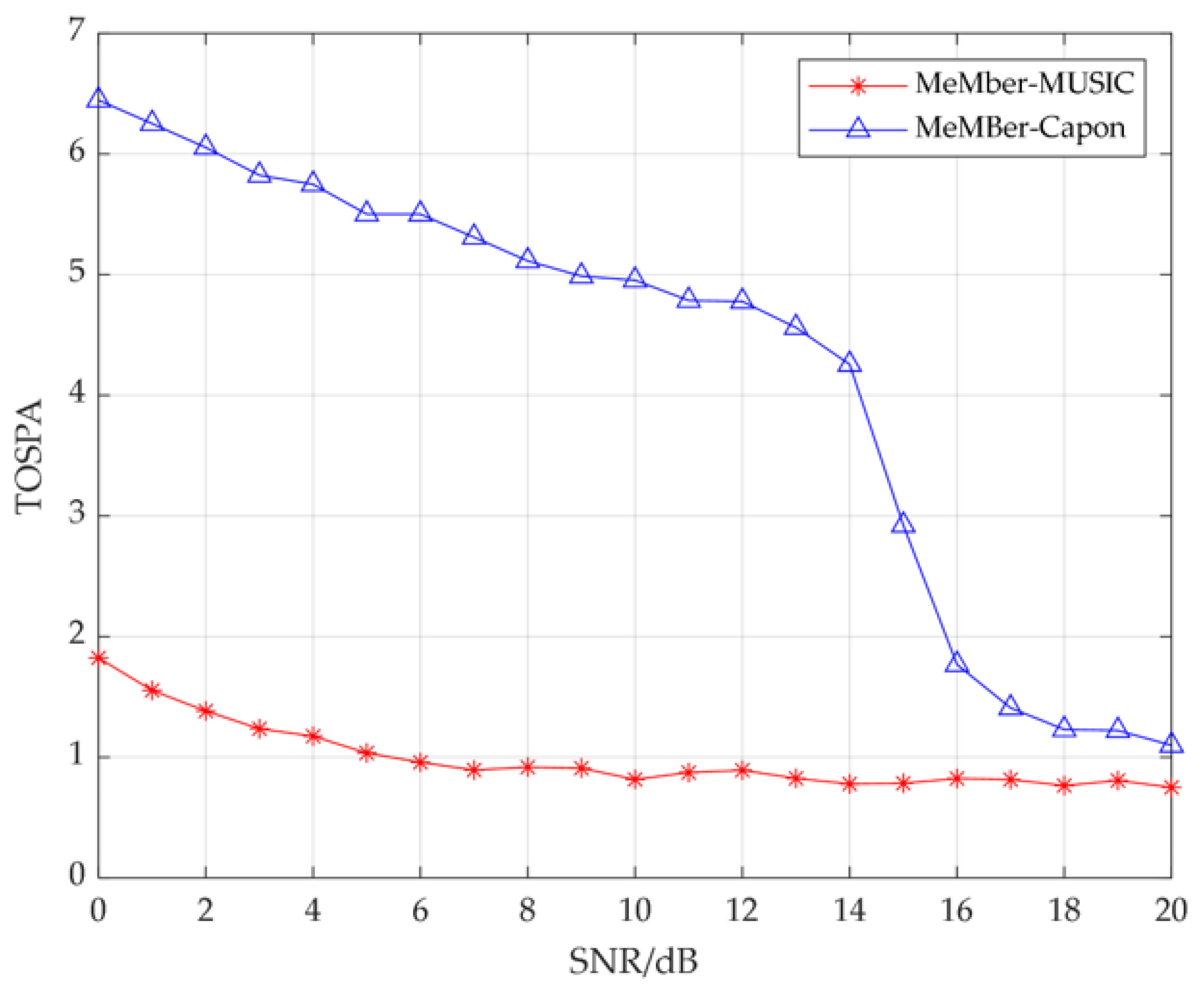
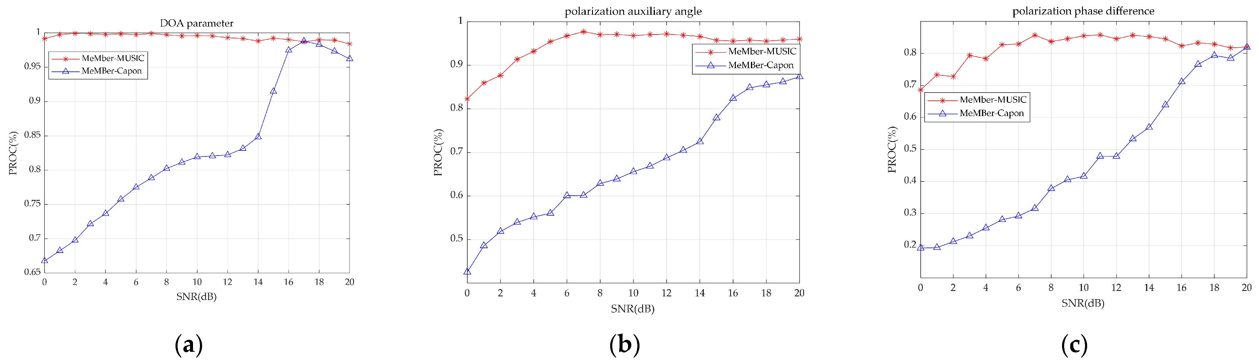
4. Simulation Analysis

To effectively assess the algorithm’s performance, the algorithm Root Mean Square Error (RMSE) is used as an indicator for evaluating the testing algorithm. RMSE is computed as the square root of the mean of the squared differences between the predicted and true values, divided by the total number of observations Monte Carlo (MC). It serves as a measure of the deviation between the observed and true values, and it can be defined as follows:
RMSE = 1 G g = 1 G 1 M C j = 1 M C ( 1 T t = 1 T ( x g , j ( t ) x ^ g , j ( t ) ) 2 ) ,
where x k , j ( n ) and x ^ k , j ( n ) represent the true and estimated values, respectively. In the j th MC simulation experiment, at time n for the k th  target signal source, where  represents the observation time, M C represents the total number of Monte Carlo simulations, and K represents the estimated number of signal sources.
Probability of Convergence (PROC) signifies the likelihood that the deviation between the observed and true values remains within a specified range, thus indicating the convergence ability of the observed value. PROC can be defined as follows:
P R O C = 1 T t = 1 T j = 1 M C 1 t , j / M C × 100 % ,
where the coefficient 1 t , j can be determined as follows:
1 t , j = { 1 , | x j ( t ) x ^ j ( t ) | < ε 0 ,   other
Additionally, this study introduces Optimal Subpattern Assignment (OSPA) error as a metric for evaluating performance. OSPA error serves the purpose of estimating the discrepancy between the target state and the true state while also quantifying the penalty incurred when an existing source is overlooked or when a non-existent source is incorrectly detected. OSPA is widely used in assessing and evaluating the performance of multi-target filtering problems. OSPA error can be defined as follows:
d ¯ p ( c ) ( X , Y ) = ( 1 n ( min π Π n i = 1 m d ( c ) ( x i , y π ( i ) ) p + c p ( n m ) ) ) 1 p
d ( c ) ( x , y ) = min ( c , d ( x , y ) ) ,
where d ( x , y ) = x y represents the distance between x and y and x represents the true value and y represents the estimated value. The sets X = { x 1 , x 2 , , x m } and Y = { y 1 , y 2 , , y n } represent the true set and the estimated set, respectively. m and n represent the true number and the estimated number of elements, respectively. c represents the penalty parameter, p is the order parameter and Π n represents a set that selects m elements from the set { 1 , 2 , , n } and arranges them.

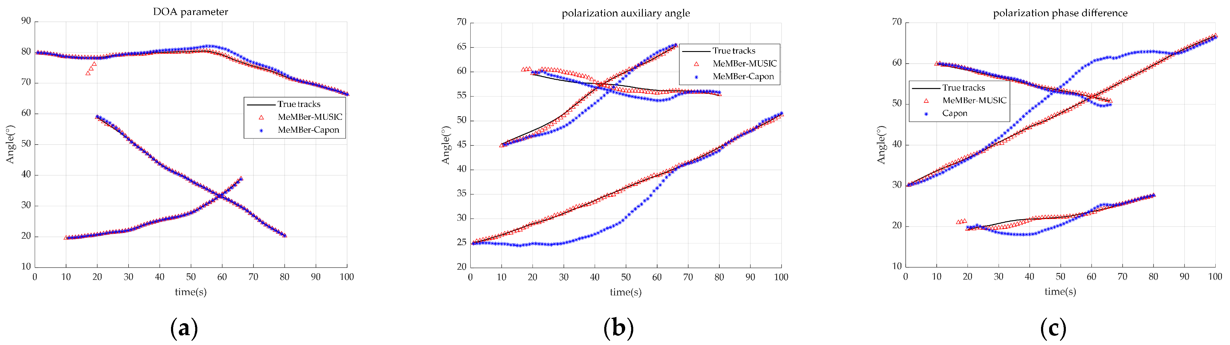
4.1. Joint DOA-Polarization Parameter Tracking with the Fixed Source Number

The operating environment includes an AMD Ryzen 7 [email protected] GHz and a 64-bit operation system MATLAB 2022. In Simulation 1, the conditions are as follows: The number of array elements is M = 10. The number of fast beats of the received signal is L = 100. Signal-to-Noise Ratio (SNR) is 15 dB. The observation time is 100 s. The time step is ΔT = 1 s. The number of signal sources is 3, and the states change with time. The initial states of the signal sources are x1 = [69.9, −0.09, 30.3, 0.31, 25.1, 0.11]T, x2 = [19.6, −0.17, 59.9, −0.14, 45.2, 0.24]T and x3 = [58.8, −0.73, 19.2, 0.19, 59.4, −0.07]T. The source survival probability is ps,k = 0.98. In the prediction stage of the MeMBer joint DOA-polarization parameter tracking algorithm, it is assumed that there are three new signal sources at every moment, denoted as JB,K = 3. Each new signal source generates 1000 particles, denoted as NB,K = 1000.
Figure 2 presents a Monte Carlo trajectory tracking diagram of three signal sources under an SNR of 15 dB. The results indicate that the PAST algorithm demonstrates superior tracking performance in the spatial domain compared to the polarization domain. However, when the spatial parameters are closely spaced, the estimated values tend to converge towards the DOA of similar signal sources, leading to inaccurate estimations. Conversely, the PAST algorithm experiences larger tracking errors in the polarization domain. Similarly, the MeMBer—Capon algorithm encounters significant estimation errors in the polarization domain during the tracking process. In contrast, the proposed joint DOA-polarization parameter MeMBer—MUSIC tracking algorithm exhibits estimations that are closer and less deviated from the true values, particularly for tracking fast-moving targets. Consequently, it outperforms PAST and MeMBer—Capon algorithms. In Figure 3, the joint mean square error diagram portrays 100 Monte Carlo tests for three signal sources under an SNR of 15 dB. The results illustrate that the proposed MeMBer—MUSIC algorithm demonstrates greater robustness and accuracy in estimating the state of signal sources compared to MeMBer—Capon algorithm. The tracking estimation performance of the proposed algorithm for joint DOA-polarization parameters initially improves with time, followed by a rapid decrease in error. Furthermore, the proposed algorithm exhibits lower mean square error, less time fluctuation and enhanced robustness in comparison to the MeMBer—Capon algorithm. Consequently, the proposed joint DOA-polarization parameter MeMBer—MUSIC algorithm provides estimations that are closer to the true values and yields a smaller RMSE compared to the traditional MeMBer—Capon algorithm.
The joint RMSE of the aforementioned algorithms, as SNR changes, is illustrated in Figure 4. A total of 100 Monte Carlo experiments were conducted for each SNR ranging from 0 to 20 dB . From Figure 4, it can be observed that as SNR increases, the RMSE of the joint DOA-polarization parameter algorithm decreases for the spatial parameter. Similarly, a decreasing trend in RMSE is observed for the polarization parameter with higher SNR values. Notably, across different SNRs, the RMSE of the proposed joint DOA-polarization parameter MeMBer—MUSIC algorithm is significantly smaller than that of MeMBer—Capon algorithm. Even under low SNRs, the proposed algorithm maintains high tracking accuracy, while MeMBer—Capon algorithm experiences larger errors and lower tracking accuracy.
Table 1 presents memory usage and average processing time per time instant for different algorithms. From Table 1, it can be observed that the MeMBer—MUSIC algorithm falls between the MeMBer—Capon algorithm and the PAST algorithm in terms of memory usage and average processing time per frame. The three algorithms occupy similar memory, but the MeMBer—MUSIC algorithm requires much less time on average per time instant compared to the PAST algorithm, and it is comparable to the MeMBer—Capon algorithm. Combining the comprehensive analysis of the RMSE in the simulation experiments between the algorithms, the MeMBer—MUSIC algorithm exhibits higher tracking accuracy than the MeMBer—Capon algorithm, despite having similar memory usage and average processing time per time instant.

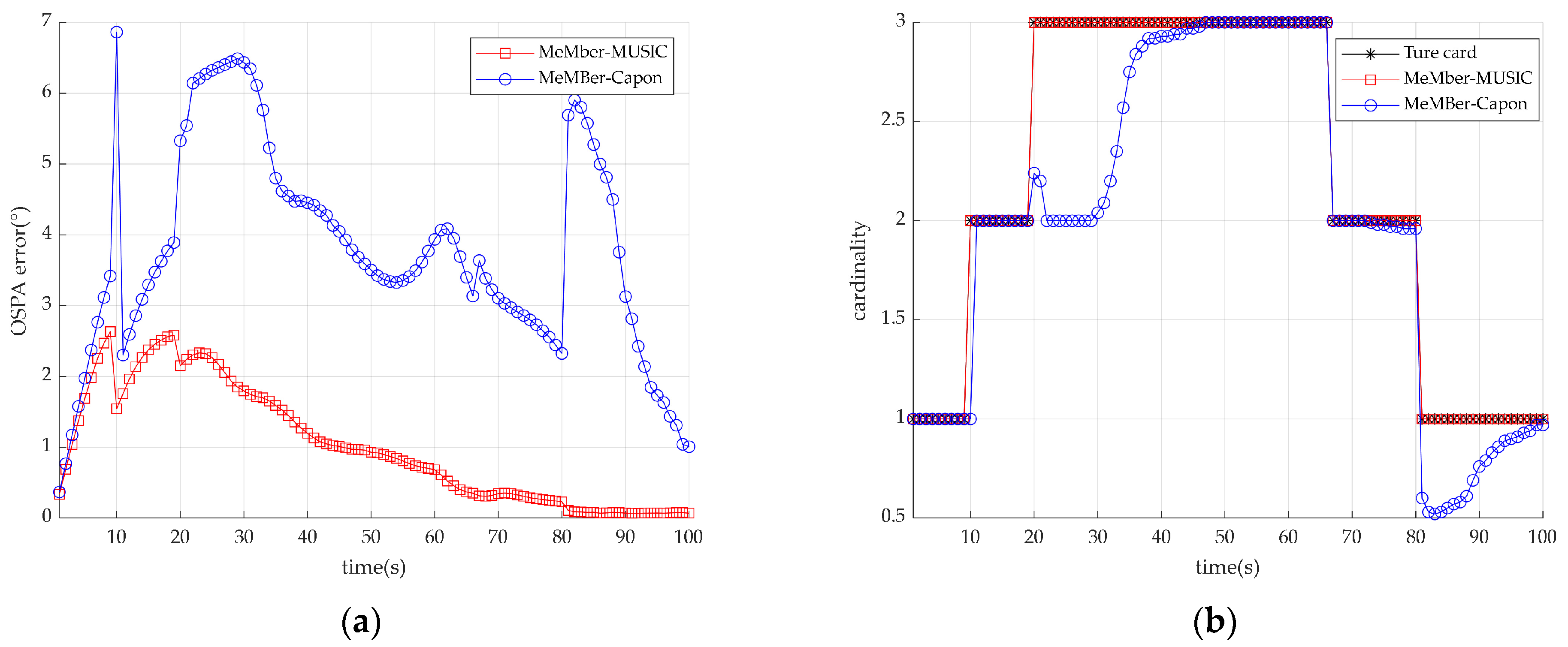
4.2. Joint DOA-Polarization Parameter Tracking with the Time-Varying Source Number

The simulation is conducted under the following conditions: the number of array elements is M = 10, the number of received signal snapshots is L = 1000, SNR is 15 dB, the observation time is T = 100 s and the time step is ΔT = 1 s. The scenario involves multiple signal sources with varying status and number of sources over time. Table 2 presents the time of birth and death of signal sources, along with their respective status.
The trajectory tracking diagram in Figure 5 illustrates the results obtained through Monte Carlo experiments involving three signal sources under an SNR of 15 dB. As shown in Figure 5, it is evident that the proposed algorithm achieves superior accuracy in tracking the status of signal sources compared to the MeMBer—Capon algorithm. The estimated values obtained by the proposed algorithm exhibit consistent fluctuations around the true angle, enabling timely detection of the signal source even when it momentarily disappears. In contrast, under the same simulation conditions, the MeMBer—Capon algorithm exhibits large estimation errors, particularly in tracking parameters in the polarization domain. This results in substantial deviations from the true state of the signal source. Overall, the joint DOA-polarization parameter MeMBer—MUSIC algorithm outperforms MeMBer—Capon algorithm in accurately tracking signal sources.
To provide a comprehensive evaluation of the MeMBer—MUSIC algorithm and MeMBer—Capon algorithm, a total of 100 Monte Carlo experiments were conducted on three signal sources. OSPA error was selected as a measure to assess the performance of the multi-target filtering tracking algorithms. OSPA error diagram of the joint DOA-polarization parameter MeMBer—MUSIC algorithm and MeMBer—Capon algorithm under an SNR of 15 dB, with order parameter p = 1 and penalty parameter c = 10°, is illustrated in Figure 6a. It can be observed that the OSPA error of the MeMBer—MUSIC algorithm experiences a significant increase when the signal source appears. However, when considering the overall performance, the algorithm achieves significantly smaller OSPA errors compared to the MeMBer—Capon algorithm. Furthermore, Figure 6b illustrates the potential estimation diagram after 100 Monte Carlo experiments on three signal sources. It is evident that the proposed MeMBer—MUSIC algorithm accurately estimates the number of signal sources, even when the number of sources changes over time and when targets appear or disappear. The potential estimation closely aligns with the actual number of sources, indicating the algorithm’s effectiveness in adaptively tracking the varying number of signal sources. In contrast, the MeMBer—Capon algorithm demonstrates poor performance in potential estimation, consistently underestimating the number of signal sources. Based on the results of the 100 Monte Carlo experiments, it is evident that the proposed MeMBer—MUSIC algorithm outperforms the MeMBer—Capon algorithm in terms of tracking effectiveness, as evidenced by the smaller OSPA errors and more accurate potential estimation.
Temporal OSPA (TOSPA) angle error diagram, depicting the average OSPA error over time between the estimated and true values obtained by the MeMBer—MUSIC algorithm and MeMBer—Capon algorithm under various SNRs, is presented in Figure 7. For each SNR in the range of 0–20 dB, a total of 100 Monte Carlo experiments were conducted. In Figure 7, it is evident that as SNR increases, OSPA angle error decreases for both the MeMBer—MUSIC algorithm and the MeMBer—Capon algorithm. However, the proposed algorithm consistently exhibits smaller OSPA angle errors compared to the MeMBer—Capon algorithm across different SNRs. These findings support the conclusion that the proposed MeMBer—MUSIC algorithm exhibits superior tracking performance in comparison to the MeMBer—Capon algorithm, as demonstrated by the results of the 100 Monte Carlo experiments conducted under different SNRs.
PROC graph obtained by MeMBer—MUSIC algorithm and MeMBer—Capon algorithm under different SNRs is depicted in Figure 8. The PROC graph serves as an indicator to evaluate the tracking convergence of the two algorithms. A total of 100 Monte Carlo experiments were performed for each SNR ranging from 0 to 20 dB. In Figure 8, it is observed that as SNR increases, both the MeMBer—MUSIC algorithm and the MeMBer—Capon algorithm exhibit higher PROC values. Notably, the algorithm proposed in this study consistently demonstrates a higher probability of tracking convergence even at lower SNRs. Furthermore, in both the spatial and polarization domains, the proposed algorithm shows higher tracking convergence probabilities compared to the MeMBer—Capon algorithm. In conclusion, the proposed DOA-polarization MeMBer—MUSIC algorithm outperforms the MeMBer—Capon algorithm in terms of tracking performance.

5. Conclusions

This study proposes a joint DOA-polarization joint parameter tracking algorithm based on the MeMBer filter. The algorithm leverages the MDL principle to adaptively estimate the number of signal sources and partition the subspaces. In the MeMBer update step, the likelihood function is computed using the peak characteristics of the joint parameter MUSIC spatial spectrum function. SMC implementation method for the algorithm is provided in this research. The results demonstrate that the proposed algorithm exhibits higher tracking accuracy compared to the MeMBer—Capon algorithm and PAST algorithm in scenarios with a fixed number of signal sources. Furthermore, it maintains lower tracking errors under low SNRs. In scenarios where the number of signal sources varies over time, the proposed method successfully tracks joint DOA-polarization parameters and exhibits lower OSPA errors, providing more accurate estimates of potential targets.
The proposed DOA-polarization joint parameter tracking algorithm is implemented within the MeMBer filtering framework, enabling effective estimation of the number and states of signal sources. However, it should be noted that the algorithm requires a high snapshot count. As the real-time requirements for DOA and polarization parameter estimation continue to increase, future research can focus on extending DOA-polarization joint parameter tracking to lower snapshot counts. This would improve the real-time estimation of signal source states while mitigating the performance degradation caused by spatial spectrum expansion.

Author Contributions

Conceptualization, Z.C. and B.W.; methodology, B.W.; software, B.W. and Z.C.; validation, B.W., Z.C. and R.Y.; writing—original draft preparation, B.W., Z.C., R.Y. and Y.L.; writing—review and editing, B.W. and Z.C. All authors have read and agreed to the published version of the manuscript.

Funding

This research was funded by the Natural Science Foundation of China (grant nos. 61701148).

Data Availability Statement

Not applicable.

Conflicts of Interest

The authors declare no conflict of interest.

References

  1. Schmidt, R. Multiple emitter location and signal parameter estimation. IEEE Trans. Antennas Propag. 1986, 34, 1668–1676. [Google Scholar] [CrossRef] [Green Version]
  2. Ateşavcı, C.S.; Bahadırlar, Y.; Aldırmaz-Çolak, S. DoA Estimation in the Presence of Mutual Coupling Using Root-MUSIC Algorithm. In Proceedings of the 2021 8th International Conference on Electrical and Electronics Engineering (ICEEE), Antalya, Turkey, 9–11 April 2021. [Google Scholar]
  3. Yin, D.; Zhang, F. Uniform linear array MIMO radar unitary root MUSIC Angle estimation. In Proceedings of the 2020 Chinese Automation Congress (CAC), Shanghai, China, 6–8 November 2020. [Google Scholar]
  4. Li, J.; Li, D.; Jiang, D.; Zhang, X. Extended-Aperture Unitary Root MUSIC-Based DOA Estimation for Coprime Array. IEEE Commun. Lett. 2018, 22, 752–755. [Google Scholar] [CrossRef]
  5. Roy, R.; Kailath, T. ESPRIT-estimation of signal parameters via rotational invariance techniques. IEEE Trans. Acoust. Speech Signal Process. 1989, 37, 984–995. [Google Scholar] [CrossRef] [Green Version]
  6. Stoica, P.; Nehorai, A. MUSIC, maximum likelihood and Cramer-Rao bound. IEEE Trans. Acoust. Speech Signal Process. 1989, 37, 720–741. [Google Scholar] [CrossRef]
  7. Meng, D.; Wang, X.; Huang, M.; Wan, L.; Zhang, B. Robust Weighted Subspace Fitting for DOA Estimation via Block Sparse Recovery. IEEE Commun. Lett. 2020, 24, 563–567. [Google Scholar] [CrossRef]
  8. Tong, Y.; Zuo, W.; Xin, J.; Zheng, N.; Sano, A. Direction-of-Arrival and Range Estimation of Near-Field Sources Based on Subspace Fitting. In Proceedings of the 2021 China Automation Congress (CAC), Beijing, China, 22–24 October 2021. [Google Scholar]
  9. Yang, B. Projection approximation subspace tracking. IEEE Trans. Signal Process. 1995, 4, 95–107. [Google Scholar] [CrossRef]
  10. Orton, M.; Fitzgerald, W. A Bayesian approach to tracking multiple targets using sensor arrays and particle filters. IEEE Trans. Signal Process. 2002, 50, 216–223. [Google Scholar] [CrossRef]
  11. Mahler, R.P.S. Multitarget Bayes filtering via first-order multitarget moments. IEEE Trans. Aerosp. Electron. Syst. 2003, 39, 1152–1178. [Google Scholar] [CrossRef]
  12. Vo, B.T.; Vo, B.N. A random finite set conjugate prior and application to multi-target tracking. In Proceedings of the 2011 Seventh International Conference on Intelligent Sensors, Sensor Networks and Information Processing, Adelaide, SA, Australia, 6–9 December 2011. [Google Scholar]
  13. Vo, B.T.; Vo, B.N.; Cantoni, A. Analytic Implementations of the Cardinalized Probability Hypothesis Density Filter. IEEE Trans. Signal Process. 2007, 55, 3553–3567. [Google Scholar] [CrossRef]
  14. Nannuru, S.; Coates, M.; Mahler, R. Computationally-Tractable Approximate PHD and CPHD Filters for Superpositional Sensors. IEEE J. Sel. Top. Signal Process. 2013, 7, 410–420. [Google Scholar] [CrossRef]
  15. Saucan, A.A.; Chonavel, T.; Sintes, C. CPHD-DOA Tracking of Multiple Extended Sonar Targets in Impulsive Environments. IEEE Trans. Signal Process. 2016, 64, 1147–1160. [Google Scholar] [CrossRef]
  16. Choppala, P.B.; Teal, P.D.; Frean, M.R. Adapting the multi-Bernoulli filter to phased array observations using MUSIC as pseudo-likelihood. In Proceedings of the 17th International Conference on Information Fusion (FUSION), Salamanca, Spain, 7–10 July 2014. [Google Scholar]
  17. Wu, S.Y.; Zou, B.H.; Xue, Q.T. DOA tracking algorithm based on single snapshot spatial smoothing with multi-Bernoulli. Syst. Eng. Electron. 2021, 43, 2430–2438. [Google Scholar]
  18. Zhao, J.; Gui, R.; Dong, X.; Wu, S. Time-Varying DOA Tracking Algorithm Based on Generalized Labeled Multi-Bernoulli. IEEE Access 2021, 9, 5943–5950. [Google Scholar] [CrossRef]
  19. Zhao, J.; Gui, R.; Dong, X. A new measurement association mapping strategy for DOA tracking—ScienceDirect. Digit. Signal Process. 2021, 118, 103228. [Google Scholar] [CrossRef]
  20. Ferrara, E.; Parks, T. Direction finding with an array of antennas having diverse polarizations. IEEE Trans. Antennas Propag. 1983, 31, 231–236. [Google Scholar] [CrossRef]
  21. Wong, K.T.; Zoltowski, M.D. Self-initiating MUSIC-based direction finding and polarization estimation in spatio-polarizational beamspace. IEEE Trans. Antennas Propag. 2000, 48, 1235–1245. [Google Scholar]
  22. Yuan, Q.W.; Chen, Q.; Sawaya, K. MUSIC based DOA finding and polarization estimation using USV with polarization sensitive array antenna. In Proceedings of the 2006 IEEE Radio and Wireless Symposium, San Diego, CA, USA, 17–19 October 2006. [Google Scholar]
  23. Cheng, Q.; Hua, Y.B. Further study of the Pencil-MUSIC algorithm. IEEE Trans. Aerosp. Electron. Syst. 1996, 32, 284–299. [Google Scholar] [CrossRef]
  24. Wong, K.T.; Zoltowski, M.D. Polarization-beamspace self-initiating MUSIC for azimuth/elevation angle estimation. In Proceedings of the Radar 97 (Conference Publication Number 449), Edinburgh, UK, 14–16 October 1997. [Google Scholar]
  25. Li, J.; Compton, R.T. Angle estimation using a polarization sensitive array. In Proceedings of the Antennas and Propagation Society Symposium 1991 Digest, London, ON, Canada, 24–28 June 1991. [Google Scholar]
  26. Chen, F.J.; Kwong, S.; Kok, C.W. Two-dimensional angle and polarization estimation using ESPRIT without pairing. In Proceedings of the 2006 IEEE International Symposium on Circuits and Systems (ISCAS), Kos, Greece, 21–24 May 2006. [Google Scholar]
  27. Lin, C.H.; Fang, W.H.; Yang, W.S.; Line, J.D. SPS-ESPRIT for joint DOA and polarization estimation with a COLD array. In Proceedings of the 2007 IEEE Antennas and Propagation Society International Symposium, Honolulu, HI, USA, 9–15 June 2007. [Google Scholar]
  28. Picheral, J.; Piqueres, F. Joint angle/Delay/Polarization Estimation by esprit-like method for multipath channel identification. In Proceedings of the 2004 12th European Signal Processing Conference, Vienna, Austria, 6–10 September 2004. [Google Scholar]
  29. Sam, K.; Fei, J. Frequency and 2D Angle Estimation Based on a Sparse Uniform Array of Electromagnetic Vector Sensors. Eurasip J. Adv. Signal Process. 2006, 2006, 1–9. [Google Scholar]
  30. Friedlander, B.; Weiss, A.J. A direction finding algorithm for diversely polarized arrays. Digit. Signal Process. 2000, 2, 123–134. [Google Scholar] [CrossRef]
  31. Wong, K.T.; Li, L.S.; Zoltowski, M.D. Root-MUSIC-based direction-finding and polarization estimation using diversely polarized possibly collocated antennas. IEEE Antennas Wirel. Propag. Lett. 2004, 3, 129–132. [Google Scholar] [CrossRef]
  32. Belloni, F.; Richter, A.; Koivunen, V. Performance of root-MUSIC algorithm using real-world arrays. In Proceedings of the 2006 14th European Signal Processing Conference, Florence, Italy, 4–8 September 2006. [Google Scholar]
  33. Qiu, S.; Sheng, W.; Ma, X.; Kirubarajan, T. A Maximum Likelihood Method for Joint DOA and Polarization Estimation Based on Manifold Separation. IEEE Trans. Aerosp. Electron. Syst. 2021, 57, 2481–2500. [Google Scholar] [CrossRef]
  34. Chalise, B.K.; Zhang, Y.D.; Himed, B. Compressed Sensing based Joint Doa and Polarization Angle Estimation for Sparse Arrays with Dual-Polarized Antennas. In Proceedings of the 2018 IEEE Global Conference on Signal and Information Processing (GlobalSIP), Anaheim, CA, USA, 26–29 November 2018. [Google Scholar]
  35. Shao, S.; Liu, A.; Yu, C.J.; Zhao, Q.R. Polarization quaternion DOA estimation based on vector MISC array. J. Syst. Eng. Electron. 2021, 32, 764–778. [Google Scholar]
  36. Wang, J.; Du, Y.; Chen, L.; Han, D. Fast algorithm of joint polarization and DOA estimation for irregular array under coherent sources. In Proceedings of the IET International Radar Conference (IET IRC 2020), Online Conference, 4–6 November 2020. [Google Scholar]
  37. Yue, Y.; Zhang, Z.; Zhou, C.; Xing, F.; Shi, Z. Closed-form Two-dimensional DOA and Polarization Joint Estimation Using Parallel Non-collocated Sparse COLD Arrays. In Proceedings of the 2022 IEEE 12th Sensor Array and Multichannel Signal Processing Workshop (SAM), Trondheim, Norway, 20–23 June 2022. [Google Scholar]
  38. He, Z.; Tian, Z.; Zhou, M.; Li, Z.; Liu, K. DOA Estimation Method for Polarization Sensitive Circular Array Based on Reduced-Dimensional MUSIC. In Proceedings of the 2022 IEEE International Symposium on Antennas and Propagation and USNC-URSI Radio Science Meeting (AP-S/URSI), Denver, CO, USA, 10–15 July 2022. [Google Scholar]
  39. Wax, M.; Ziskind, I. Detection of the number of coherent signals by the MDL principle. IEEE Trans. Acoust. Speech Signal Process. 1989, 37, 1190–1196. [Google Scholar] [CrossRef]
  40. Zhang, G.P.; Zheng, C.; Sun, S.B. Joint Detection and DOA Tracking with a Bernoulli Filter Based on Information Theoretic Criteria. Sensors 2018, 18, 3473. [Google Scholar] [CrossRef] [PubMed] [Green Version]
  41. Cappe, O.; Godsill, S.J.; Moulines, E. An Overview of Existing Methods and Recent Advances in Sequential Monte Carlo. Proc. IEEE 2007, 95, 899–924. [Google Scholar] [CrossRef]
  42. Vo, B.T.; Clark, D.; Vo, B.N. Bernoulli Forward-Backward Smoothing for Joint Target Detection and Tracking. IEEE Trans. Signal Process. 2011, 59, 4473–4477. [Google Scholar] [CrossRef]
Figure 1. Structure of a uniform linear polarization sensitive array structure.
Remotesensing 15 03929 g001
Figure 2. Joint DOA-polarization parameter track tracking, and L = 1000 : (a) Trajectory tracking of DOA parameter; (b) Trajectory tracking of polarization auxiliary angle; (c) Trajectory tracking of polarization phase difference.
Remotesensing 15 03929 g002
Figure 3. RMSE under SNR = 15 dB, L = 1000, and MC = 100: (a) RMSE of DOA parameter; (b) RMSE of polarization parameter.
Remotesensing 15 03929 g003
Figure 4. RMSE of joint DOA-polarization parameter tracking SNR = 0–20 dB and MC = 100: (a) RMSE of DOA parameter; (b) RMSE of polarization parameter.
Remotesensing 15 03929 g004
Figure 5. Trajectory tracking diagram, SNR = 15 dB, L = 1000 and T = 100 s: (a) Trajectory tracking of DOA parameter; (b) Trajectory tracking of polarization auxiliary angle; (c) Trajectory tracking of polarization phase difference.
Remotesensing 15 03929 g005
Figure 6. OSPA error and cardinality estimation of angle under SNR = 15 dB, p = 1 and c = 10°: (a) OSPA of joint DOA-polarization parameter; (b) Cardinality estimation of angle.
Remotesensing 15 03929 g006
Figure 7. TOSPA under different SNRs.
Remotesensing 15 03929 g007
Figure 8. PROC under different SNRs with MC = 100: (a) PROC of DOA parameter; (b) PROC of polarization auxiliary angle; (c) PROC of polarization phase difference.
Remotesensing 15 03929 g008
Table 1. Memory usage and average processing time per time instant for different algorithms.
AlgorithmsMemory UsageAverage Processing Time per Time Instant
MeMBer—MUSIC1,860,180 Kb0.14884489 s
MeMBer—Capon1,838,996 Kb0.10783062 s
PAST1,981,908 Kb0.26529525 s
Table 2. Trajectory of joint DOA-polarization parameters of signal source.
TargetSignal Source Joint DOA-Polarization Parameter Trajectory
State of BirthBirth Time/sDeath Time/s
Signal source 1 [ 79.9 , 0.07 , 30.3 , 0.35 , 25.1 , 0.15 ] T 1100
Signal source 2 [ 19.5 , 0.08 , 59.9 , 0.17 , 45.2 , 0.26 ] T 1066
Signal source3 [ 58.8 , 0.71 , 19.2 , 0.20 , 59.4 , 0.09 ] T 2080
Disclaimer/Publisher’s Note: The statements, opinions and data contained in all publications are solely those of the individual author(s) and contributor(s) and not of MDPI and/or the editor(s). MDPI and/or the editor(s) disclaim responsibility for any injury to people or property resulting from any ideas, methods, instructions or products referred to in the content.

