An Intra-Class Ranking Metric for Remote Sensing Image Retrieval

Abstract

With the rapid development of internet technology in recent years, the available remote sensing image data have also been growing rapidly, which has led to an increased demand for remote sensing image retrieval. Remote sensing images contain rich visual and semantic features, and have high variability and complexity. Therefore, remote sensing image retrieval needs to fully utilize the information in the images to perform feature extraction and matching. Metric learning has been widely used in image retrieval as it can train embedding spaces with high discriminability. However, existing deep metric learning methods learn embedding spaces with high discriminability by maximizing the differences between classes, while ignoring inherent intra-class differences during the learning process. In this paper, we design a new sample generation mechanism to generate samples from positive samples that meet the boundary constraints, thus obtaining quantifiable intra-class differences from real positive samples. Based on the sample generation relationship, we use a self-supervised approach to design an intra-class ranking loss function, which improves the discriminability of the generated embedding space for samples of the same class and maintains their ranking relationship in the embedding space. Moreover, this loss function can be easily combined with existing deep metric learning methods. Our aim is to help the network to better extract features and further improve the performance of remote sensing image retrieval through the sample generation mechanism and intra-class ranking loss. Finally, we conduct extensive experiments on multiple remote-sensing image datasets using multiple evaluation metrics such as mAP@K, which demonstrate that using the sample-generated intra-class ranking loss function can effectively improve the performance of remote sensing image retrieval.

1. Introduction

With the rapid development of remote sensing technology and the widespread availability of remote sensing devices, the quantity and types of remote sensing image data have grown exponentially. Utilizing these images to meet industry needs has become a focus of research, leading to the field of remote sensing image retrieval [1,2,3,4,5]. The primary task of remote sensing image retrieval is to search for images in a large database that are related to a given query image. This involves searching for similar images based on various visual features such as color, texture, and shape, as well as semantic features such as land cover type, land use, and object category. With the great achievements in the work on remote sensing applications [6,7,8,9,10,11], remote sensing image retrieval has also been effectively used for applications such as geolocalization, meteorological analysis, and ecological prediction [12,13,14], among other applications.

One of the main challenges in remote sensing image retrieval is the high variability and complexity of the images. Remote sensing images may vary significantly in spatial and spectral resolution, viewing angle, lighting conditions, and atmospheric effects, making it difficult to accurately compare and match images. In addition, remote sensing images often contain a large amount of background noise and clutter, which can affect the accuracy of feature extraction and matching algorithms. Another major challenge is the lack of annotated data for training and evaluation. Remote sensing images are typically large and complex, making manual annotation with ground truth information difficult and expensive. This may limit the performance of algorithms that rely on labeled data for training and evaluation. Due to their wide range of applications and excellent performance, machine learning and deep learning have been applied to many tasks [15,16,17,18,19], remote sensing image retrieval being one of them.

Human eyes can distinguish whether two original images are similar, but computers cannot do so directly. Therefore, it is necessary to transform the original images into a format that computers can “understand”. This transformation turns the images into high discriminative feature vectors, which can be used to calculate metrics such as Euclidean distance and cosine similarity, to determine whether two images are similar. However, transforming images into highly discriminative feature vectors that also retain the effective visual information of the original images is not a simple process. With the advent of deep convolutional neural networks [20], this problem has been solved. Deep convolutional neural networks can transform images into feature vectors that can be calculated by computers, while effectively retaining the visual information of the original images. However, the “effectiveness” of this transformation depends on whether the deep convolutional neural network has been trained well enough. Deep metric learning [21] can train the deep convolutional neural network to perform well and meet the goals of image retrieval tasks. The framework of deep metric-learning training and retrieval is shown in Figure 1. Deep metric learning defines the space in which the feature vectors exist as the feature embedding space, where similar samples (such as images from the same category) are grouped together, while different samples (such as images from different categories) are far apart. By designing effective loss functions and using the gradient for backpropagation, deep metric learning constrains the learning of the convolutional neural network to obtain such a feature embedding space. In this feature embedding space, images can be transformed into feature vectors that meet the needs of image retrieval tasks. The feature vectors of different categories are far apart or have a small similarity, while those of the same category are close together or have a high similarity. This enables the retrieval of similar images during the search.

The excellence of the feature embedding space determines the quality of the feature vector obtained by image conversion and the quality of the image retrieval results. Designing an effective loss function is crucial for obtaining an excellent and highly robust feature embedding space. The research of deep metric learning mainly focuses on designing an effective loss function, and the loss functions discussed in the current study can be divided into two types: pair-based loss functions and proxy-based loss functions.

In a particular embedding space, the distances between feature vectors from the same class are called intra-class differences, and the distances between feature vectors from different classes are called inter-class differences. Existing deep metric learning methods learn highly discriminative embedding spaces by maximizing inter-class differences as much as possible. However, these methods ignore the inherent intra-class differences during the learning process. Due to the lack of labels, they treat all positive samples equally and try to distinguish positive samples from negative samples, completely discarding the ranking information of different positive samples. When intra-class differences are ignored, the local structure is unconsciously destroyed, and overfitting to the training set is likely to occur, resulting in lower generalization performance on the test set. In previous methods, positive samples that satisfy training constraints are often ignored during training, but doing so only wastes the abundant information carried by positive samples.

The objective of this paper is to help the network to learn and extract features better through the sample generation mechanism and the proposed intra-class ranking loss, thus, improving the performance in remote sensing image retrieval tasks. The specific contribution is as follows:

We generated samples from positive samples that meet the boundary constraints. And generated samples are used to obtain quantifiable intra-class differences.

We also proposed an intra-class ranking loss function based on the self-supervised learning approach of sample generation. The training process using this loss function aims to generate an embedding space that has better discriminability for samples of the same class, while maintaining differentiation among different positive samples. Additionally, this loss function can be easily combined with existing deep metric learning methods.

We conducted a series of comparative and ablation experiments to verify the feasibility and effectiveness of our proposed method.

The rest of this paper consists of four parts: Section 2 discusses additional work related to our approach. Section 3 proposes a new sample generation method based on self-supervised learning methods and generative relationship, and designs an intra-class ranking loss function. Section 4 describes the dataset used for the experiment, implementation details, and metrics. Section 5 provides experimental evidence of the effectiveness of the intra-class ranking loss function in remote sensing image retrieval tasks. Section 6 summarizes the work performed in this paper.

2. Related Works

2.1. Remote Sensing Image Retrieval

Most of the existing remote-sensing image retrieval techniques are based on hash algorithms. Hashing algorithms are usually based on mapping the high dimensional features of an image into Hamming space. A low-dimensional hash sequence is used to represent an image.

Sun et al. [22] proposed a deep attention hashing algorithm with distance adaptive ordering. A distance adaptive ranking strategy is used in the retrieval phase to fully utilize the category probability information. Unlike Sun et al., Guo et al. [23] proposed a hashing method called deep adversarial cascade hashing (DACH); subsequently, deep adversarial constraints are applied to feature learning and hash learning. The method incorporates multi-level features and achieves accurate cross-modal retrieval. Tan et al. [24] proposed a deep contrast self-supervised hashing method. They designed a loss function incorporating temperature-scaled cross-entropy loss and quantization loss to train the network so as to preserve the hash codes with semantic similarity. Similarly, Sun et al. [25] proposed an unsupervised deep hashing method based on soft pseudo labels. They designed an objective function to unite soft pseudo labels and local similarity matrix.

There are also other techniques used for remote sensing image retrieval. For example, the design of networks or loss functions, and cross-domain retrieval. Hou et al. [26] present an attention-enhanced end-to-end discriminative network for content-based remote sensing image retrieval (CBRSIR) with multiscale learning. After that, they also proposed a semi-supervised approach [27], which enabled the network to learn consistent classification between the target domain and its perturbed outputs through a pseudo-label self-training and consistency regularization strategy.

2.2. Loss Functions in Deep Metric Learning

In this paper, the term “loss” corresponds to the loss function. A positive sample pair refers to two samples from the same class, while a negative sample pair refers to two samples from different classes.

2.2.1. Pair-Based Loss

Contrastive loss [28] and triplet loss [29,30,31] have been persistent topics in pair-based loss functions. Both of these losses constrain the distance between sample pairs.

The N-pair loss [32] is an extension of the triplet loss. It selects two samples from each class, one as the anchor sample and the other as the positive sample. When calculating the loss, the positive samples from other classes are used as negative samples, and then triplets are formed with the anchor sample and positive sample from the same class.

In Multi-Similarity loss, the author of [33] proposed a general pair weighting (GPW) framework to understand those pair-based loss functions and a multiple similarity loss in the framework of GPW, which is divided into two main iterative steps: mining and weighting.

Although these losses have greatly improved, there are still some issues. Firstly, too many sample pairs will lead to high training complexity and slow convergence. Secondly, too many sample pairs may significantly affect the quality of the learned embedding space. To address the training complexity issue, many pair-based losses have started to use sample mining [29,34,35,36] to select favorable sample pairs for training. Another way to avoid the impact of redundant sample pairs on the training process is to assign more weight to useful sample pairs, such as the Multi-Similarity Loss [33].

2.2.2. Proxy-Based Loss

The concept of proxy-based losses was first proposed by Proxy-NCA [37]. The purpose of this approach is to solve the sampling problem. It sets up proxies for each class, associates samples with proxies, and encourages samples to move closer to their corresponding proxies and away from other proxies.

Building on Proxy-NCA, Proxy-NCA++ loss [38] adds a temperature parameter T to make the decision boundary more accurate.

SoftTriple loss [39] is an improvement of the softmax function in proxy-based losses. It assigns multiple proxies to a class to reflect intra-class differences and adds regularization loss to multiple proxies of each class. The regularization loss is smaller for larger intra-class differences, while the regularization loss is larger for smaller intra-class differences.

The Proxy-Anchor loss [40] is designed to overcome the limitations of Proxy-NCA while maintaining low training complexity. It leverages the benefits of pair-based losses, allowing for the gradient utilization of semantic relationships between samples. Also, Proxy-Anchor loss considers all samples in a batch and weights them based on their similarity to proxies.

While the aforementioned losses can significantly reduce training complexity and speed up convergence, most of them do not utilize the rich semantic information between samples.

2.2.3. Other Methods

In addition to the traditional metric loss, many new metric loss functions have emerged in recent years. They all refer to the traditional metric losses and improve upon them.

Kan et al. [41] developed a contrastive Bayesian analysis method that proposes contrastive Bayesian losses with metric variance constraints that improve the model’s ability to generalize to new classes. Jin et al. [42] proposed a new double-weighted metric loss function by considering the metric relationship between images and labels at the image level and label category level. Saeki et al. [43] proposed a multi proxy anchor (MPA) family loss and a normalized discounted cumulative gain (nDCG@k) metric. The loss improves training capabilities while also including data features in gradient generation. Wang et al. [44] proposed a novel ranked-list loss to address the problems of existing ranked-driven structured losses. The method performs an iterative query for each instance in each mini-batch and uses the remaining instances as the set to be searched.

2.3. Sample Generation

Recently, some works [45,46,47] have proposed sample generation to produce potentially hard samples for improving the performance of deep metric learning. It aims to utilize a large number of simple negative samples and use additional pair-based relationships to train the model.

Duan et al. [46] proposed to use the idea of Generative Adversarial Networks (GANs) to learn feature representations with good discrimination. Zhao et al. [48] have a similar idea to Duan et al.; the difference is that Zhao et al. use GANs to generate hard triplets, which can help the model better learn the similarities and differences between samples. Zheng et al. [49] proposed a hardness-aware loss function, which can adaptively adjust the weights of samples based on their hardness during training, so that more difficult samples are given more weight in training. Lin et al. [47] proposed a new Variational Autoencoder (VAE) framework, which is a generative framework that can automatically learn the data distribution and has the concept of latent variables. However, it may result in harder optimization and more redundant parameters [50].

To address these issues, recent works [45,51] generate virtual samples or classes based on sample pairs and proxy-based losses through simple algebraic calculations in the embedding space.

Gu et al. [51] introduced some synthetic classes, using which can reduce the distance between classes and increase the number of samples in the same class, thus improving the performance of the model. Ko et al. [45] proposed to perform data augmentation in the embedding space, transforming samples into new ones, and training them together with the original samples as augmentation samples to increase the number of data samples to better train the model.

2.4. Self-Supervised Learning

Self-supervised learning (SSL) aims to learn discriminative feature representations [52] and embedding spaces without relying on manual annotations, by utilizing the structure or inherent correlations within the data itself. It is typically used as a pre-training process for various downstream tasks in computer vision, such as classification, detection, and segmentation. The training ability comes from various carefully designed pretext tasks, which can learn the intrinsic properties of unlabeled data. Early methods included image restoration [53] and rotation prediction [54]. Recently, contrastive self-supervised methods [52] have shown powerful performance, approaching or even surpassing traditional supervised learning. Their paradigm is defined based on pairwise relationships, similar to loss functions based on sample pairs in deep metric learning. Self-supervised learning is a kind of unsupervised learning; it does not need to acquire data annotation before training, but mines image features from unannotated images by auxiliary tasks. Therefore, self-supervised learning performs well in some tasks with little or no data annotation. Additionally, self-supervised learning helps to solve some specific problems [55], and metric learning also uses its ideas to obtain more distinctive embedding vectors [56,57].

2.5. Intra-Class Differences

Intra-class differences are usually found in the retrieval of fine-grained image datasets. This is because one of the characteristics of fine-grained image datasets is small inter-class differences and large intra-class differences. Most of the existing research has been devoted to narrowing intra-class differences and expanding inter-class differences.

Zhu et al. [58] proposed a two-path stacked attention network, where they achieved the effect of suppressing intra-class differences by segmenting the features extracting the critical regions of the image and ignoring irrelevant regions. Lu et al. [59] proposed an FGVC method based on self-attentive feature fusion and graph-propagation, which mines the granular features of an image through a feature map on one hand, and investigates the intrinsic semantic correlation between regional features on the other. Zhang et al. [60] proposed a robust perspective-sensitive network (PSNet) to learn multiple viewpoint spaces; they used perspective-sensitive RoI pools and loss functions to achieve sensitive learning. Yang et al. [61] proposed a task-specific meta-learning framework (TSMLF). They used the idea of maximizing the inter-class distance and minimizing the intra-class distance, and set a distance constraint on the intra-class distance. Alipour et al. [62] proposed a classification method based on an improved Inception V4 network. Shallow features are fused in the basic feature extraction stage. After that, the basic fusion features are weighted using multi-scale features. Zhang et al. [63] designed a bilinear convolutional neural network (BCNN), and they added marginal values to the decision boundary through the AM-Softmax function to better expand the inter-class differences and reduce the intra-class differences.

These studies have not paid attention to the feature information contained in the intra-class differences and certainly did not utilize this information to help the network extract image features.

3. Proposed Method

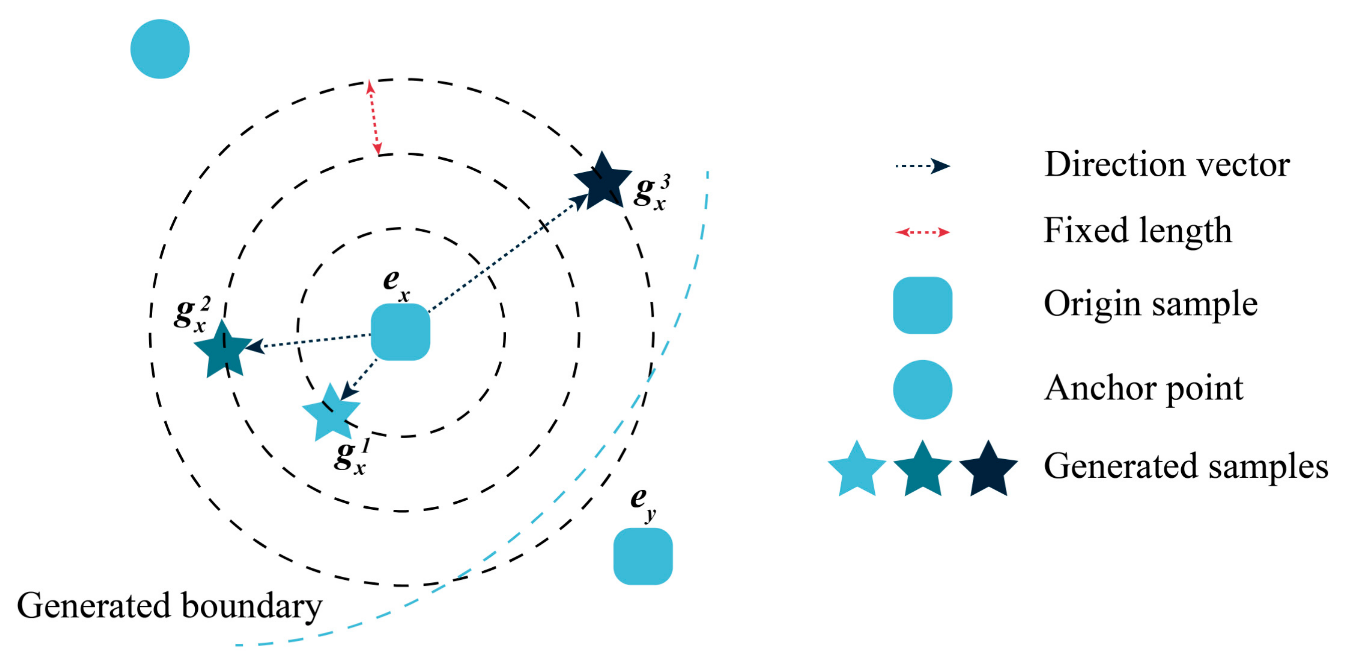
3.1. Background and Motivation for Sample Generation and Intra-Class Ranking Loss

The paradigm of deep metric learning focuses on designing appropriate loss functions that aim to minimize the distances between positive sample pairs and maximize the distances between negative sample pairs. Past deep metric learning methods learned highly discriminative embedding spaces by maximizing inter-class differences during training, but ignoring the intrinsic intra-class variations. Due to the lack of labels, these methods treated all positive samples equally during training and attempted to differentiate positive samples from negative ones, disregarding the relative ranking of different positive samples and ignoring intra-class variations, leading to the unintentional destruction of local structures. If there are multiple positive samples, the embedding vectors produced by these methods find it difficult to obtain excellent ranking results in image retrieval, and the local structure of the embedding space cannot be fully utilized due to the lack of relative ranking information. When intra-class variations are ignored, the model is prone to overfit the training set, resulting in low generalization performance on the test set.

Furthermore, in past methods, for positive samples, if they satisfy certain constraints (such as boundaries) with anchor points (which can be proxies or samples), their contribution to the model training is minimal. However, the positive samples’ handling mechanism in this approach wastes a lot of information carried by positive samples.

Therefore, addressing the above two points, this chapter proposes an intra-class ranking loss function based on a samples’ generation mechanism, which generates positive samples that meet certain conditions to obtain quantifiable intra-class variations from real positive samples. Deep networks can learn high-level representations with abstract semantics and map images to a high-dimensional feature embedding space. Different unit direction vectors in this space correspond to different semantic transformations. Generated samples are generated based on the embedding vector of real samples and direction vectors of different lengths, where the length of the direction vector represents the strength of the semantics and the direction of the direction vector represents the rich semantic diversity, that is, the intra-class variation.

Based on the generated relationship of the generated samples, this chapter designs an intra-class ranking loss function using the idea of self-supervision, which improves the discriminability of the generated embedding space for samples of the same class and maintains their ranking relationship in the embedding space, as shown in Figure 2. The ranking relationships between the generated positive samples are used to constrain the intra-class differences. The embedding space obtained in this way not only maintains the separability between classes but also distinguishes subtle intra-class differences, providing a better global and local structure for retrieval and ranking.

3.2. Image Retrieval Using the Intra-Class Ranking Loss Function Based on Sample Generation

3.2.1. Sample Generation

First, we define a batch of data as $D_t={\{a_i,c_i\}}_{i=1}^B$, a total of B samples, where $c_i\in \{1, 2,\dots , C\}$, and C represents the number of labels. $e_x$ is the embedding vector of the sample $a_x$, $e_x=f \left(a_x, \theta \right)$, f is the backbone network used for feature extraction, and $\theta$ is a parameter of the network f. The high-dimensional space where all the feature vectors are located is the feature embedding space. Since the sample generation takes place at the vector level, later on we use an embedding vector $e_x$ to represent the original sample, instead of $a_x$. $S_{x,y}$ denotes the similarity of samples $e_x$ and $e_y$. If $c_x=c_y$, then $S_{x,y}$ describes intra-class similarity and its opposite indicates intra-class differences. If $c_x\ne c_y$, then $S_{x,y}$ describes inter-class similarity and its opposite denotes inter-class differences.

The main contribution of this section is the design of a new sample generation mechanism. Most existing methods separate positive and negative samples by setting boundaries for each anchor point to attract positive samples and exclude negative samples. However, this brute-force separation method does not consider the relationship between positive samples, which can lead to insufficient differentiation among positive samples and result in an embedding space that is not sufficiently discriminative for samples of the same class. Previous methods often ignore positive samples that meet boundary constraints, which do not contribute to training. However, this approach also ignores the variety of information brought by positive samples. This chapter uses the ignored positive samples to generate a series of samples according to a certain generation rule and constructs an intra-class ranking loss function based on the generation rule to make up for the lack of discriminability among samples of the same class. The proposed method in this chapter only uses the original sample embedding vector and direction vector to generate samples without any additional generation network.

The sample generation mechanism is shown in Figure 3. During training, samples are input into the backbone network to obtain the embedding vector of the sample, and the cosine similarity between the embedding vector and the anchor point is calculated. If the similarity between the embedding vector and the anchor point is greater than m, the sample is generated. Samples that do not meet the boundary constraints (hard positive samples), such as the original sample $e_y$, will not be used to generate samples, while samples that meet the boundary constraints, such as the original sample $e_x$(easy positive samples), will generate samples. Original samples are the samples that were originally in the dataset during a training session. Generated samples are the samples obtained by the sample generation mechanism, which do not originally exist in the dataset.

For a positive sample $e_x$ that satisfies the above conditions, N samples can be generated and the generated equation is $g_x^n=e_x+\left(nr\right)u_n,$ where r denotes a fixed length, n is a positive integer from 0 to N, and nr denotes the length of the generated radius. $u_n$ is a unit vector whose direction conforms to a normal distribution, and the generation direction is controlled by $u_n$, so that we can generate a sufficient number of sparse samples and ensure the generality of the generated samples. The generated samples will be mapped by $g_{\theta }$. In the early stages of training, the ranking relationships of the mapped samples will be corrupted. We design the loss function to constrain the ranking relationship formed by the sample generation process. The sample generation method proposed by us draws on the method proposed by Fu et al. [64], but there are several differences: firstly, we only use samples that meet the generation conditions; secondly, the direction vectors are composed of additional network parameters that can be part of the neural network and continuously learned and updated during training, without the need for additional constraints; finally, the dimension of the direction vectors used for sample generation is consistent with the dimension of the sample embedding vectors, making sample generation simple.

3.2.2. Intra-Class Ranking Loss Function

Figure 3 shows that sample generation is based on the direction vector and the original sample, and the generated samples have a certain hierarchical relationship. According to this hierarchy, the ranking information between the generated samples can be clearly defined; accordingly, the generated sample $g_x^1$, which is closer to the original sample, has a higher similarity than generated sample $g_x^3$, which is further away from the original sample, i.e., S1 > S3, corresponding to${|R}_3|>\left|R_1\right|$in the figure. This ranking relationship is disrupted after projection, and a loss function is needed to maintain this relationship, so we design an intra-class ranking loss function based on this:

$$L_{\mathit{intra}-\mathit{\text{ranking}}}=\frac{1}{\left|P^{+}\right|}\sum _{p\in P^{+}}\sum _{x\in X_p^{*}}\sum _{i=1}^N\left(\mathit{log}\left(1+\sum _{j=1}^{i-1}{e}^{\alpha (-S_{j,x}+S_{i,x}+\beta )}+\sum _{j=i+1}^N{e}^{-\alpha (-S_{j,x}+S_{i,x}- \beta )}\right)\right)$$

(1)

$$L_{\mathit{gen}-\mathit{anchor}}=\frac{1}{\left|P^{+}\right|}\sum _{p\in P^{+}}\sum _{x\in X_p^{*}}\left(\mathit{log}(1+\sum _{i=1}^N{e}^{\alpha (\delta -S_{i,p})})\right)$$

(2)

$$L_{\mathit{gen}}=L_{\mathit{intra}-\mathit{ranking}}+L_{\mathit{gen}-\mathit{anchor}}$$

(3)

$P^{+}$ represents the set of all anchor points (proxy or sample) in the batch, and ${|P}^{+}|$ represents the number of all anchor points. For each anchor point p, $X_p^{*}$ is the set of samples that satisfy the generation condition, N is the number of generated samples, α > 0 is used to control the strength of pushing and pulling generated samples, β > 0 represents the similarity constraint that needs to be satisfied between generated samples, δ > 0 represents the similarity constraint that needs to be satisfied between generated samples and anchor points, and S represents the cosine similarity.

$L_{\mathit{intra}-\mathit{ranking}}$ is used to constrain the similarity between generated samples, $S_{n,x}$ represents the similarity between the generated sample $g_x^n$ and the original positive sample $e_x$. According to the sample generation description above, for all generated samples of the positive sample $e_x$, the larger the n, the smaller $S_{n,x}$ should be. Specifically, this chapter gives the following constraint: for generated sample $g_x^i$, it is agreed that when $j\in [1,i-1]$, $S_{j,x}-S_{i,x}>\beta ,\beta >0$, and when $j\in [i+1,N]$, $S_{i,x}-S_{j,x }>\beta ,\beta >0,\beta$ represents the degree of separation between adjacent generated samples. This setup allows the generated sample $g_x^i$ to associate with all generated samples, so that the ranking relations formed during the sample generation process still hold after the projection.

At the same time, the relationship between generated samples and anchor points needs to be considered, $S_{n,p}$ represents the similarity between the generated sample $g_x^n$ and the anchor point p corresponding to the positive sample $e_x$. $L_{\mathit{gen}-\mathit{anchor}}$ is used to constrain the similarity between generated samples and anchor points, so that $S_{n,p}>\delta ,\delta >0$. And $L_{\mathit{gen}}$ is the intra-class ranking loss function, which includes $L_{\mathit{intra}-\mathit{ranking}}$ and $L_{\mathit{gen}-\mathit{anchor}}$.

In the above two losses, $L_{\mathit{intra}-\mathit{ranking}}$ constrains the ranking relationship between the generated samples and $L_{\mathit{gen}-\mathit{anchor}}$ constrains the similarity between the generated samples and the anchors. In addition to this, for the original positive and negative samples, we use Proxy-Anchor loss to constrain the inter-class differences, the total loss function is as follows:

$$L_{\mathit{Proxy}-\mathit{Anchor}+\mathit{gen}}=L_{\mathit{Proxy}-\mathit{Anchor}}+\lambda L_{\mathit{gen}}$$

(4)

It is worth noting that the $L_{\mathit{Proxy}-\mathit{Anchor}}$ constrains the similarity between the anchor and the positive samples, while the $L_{\mathit{gen}-\mathit{anchor}}$ constrains the similarity between the anchor and the generated samples. There is no duplication of function between these two losses.

Self-supervised methods compose intra-class samples by constructing generating samples, and then realize the construction of the embedding space by bringing the intra-class samples closer together and pushing the samples of different classes further apart. In this paper, we utilize a similar idea by selecting eligible original samples for augmentation to generate a certain number of intra-class samples. Unlike traditional self-supervised methods, instead of emphasizing that the features of these generated samples conform to the characteristics of the intra-class distribution, we construct a more discriminative embedding space by describing the ordering properties of the features of these intra-class samples.

The entire training framework is shown as Figure 4. In the training stage, input samples are batch-sampled from the training set and fed into the backbone network to generate sample embedding vectors containing deep semantic information. For embedding vectors that satisfy the conditions for generating samples, they are input to the sample generators, and then the generated samples are transformed through a fully connected layer $g_{\theta }$. The intra-class ranking loss function is then calculated for these vectors based on the generated sample information. In addition to the intra-class ranking loss function, all samples need to be constrained by deep metric learning losses, such as Proxy-Anchor loss, Multi-Similarity loss, etc. The intra-class ranking loss function based on sample generation only serves as an auxiliary role to adjust existing metric learning loss functions and can be easily combined with Proxy-Anchor loss to help the network training. The total loss is obtained by combining the intra-class ranking loss and metric loss, and then gradient descent methods such as SGD or Adam are used to backpropagate the loss to update the neural network parameters. By repeating the above training process continuously, the loss value of the network model gradually approaches 0 until it finally converges to a stable state.

3.2.3. Gradient Analysis

To deepen the understanding of the learning process of the embedding space, this section gives the gradient of similarity between the generated samples and the original samples and the gradient of similarity between the generated samples and the anchor points in the intra-class ranking loss function. The gradient analysis is used to demonstrate the effectiveness of the intra-class ranking loss function. The gradient of the similarity between the generated samples and the original samples can be expressed as:

$$\begin{array}{l}\frac{{\partial L}_{\mathit{intra}-\mathit{ranking}}}{\partial S_{i,x}}\\ =\frac{1}{\left|P^{+}\right|}{\displaystyle \sum _{p\in P^{+}}}\left(\frac{\sum _{j=1}^{i-1}{\alpha e}^{\alpha \left(-S_{j,x}+S_{i,x}+\beta \right)}-\sum _{j=i+1}^N\alpha e^{-\alpha \left(-S_{j,x}+S_{i,x}-\beta \right)}}{1+\sum _{j=1}^{i-1}{e}^{\alpha \left(-S_{j,x}+S_{i,x}+\beta \right)}+\sum _{j=i+1}^N{e}^{-\alpha \left(-S_{j,x}+S_{i,x}-\beta \right)}}\right)\\ =\frac{1}{\left|P^{+}\right|}{\displaystyle \sum _{p\in P^{+}}}\left(\frac{g\left(i,x\right)}{1+\sum _{j=1}^{i-1}{e}^{\alpha \left(-S_{j,x}+S_{i,x}+\left(i-j\right)\beta \right)}+\sum _{j=i+1}^N{e}^{-\alpha \left(-S_{j,x}+S_{i,x}+\left(i-j\right)\beta \right)}}\right)\end{array}$$

(5)

From the gradient of the similarity between generated sample $g_x^i$ and original sample $e_x$, it can be seen that the similarity $S_{i,x}$ between generated sample $g_x^i$ and original sample $e_x$ is determined by all generated samples together. It is defined in this paper that:

$$h(i,x)=\sum _{j=1}^{i-1}{\alpha e}^{\alpha (-S_{j,x}+S_{i,x}+\beta )}-\sum _{j=i+1}^N\alpha e^{-\alpha (-S_{j,x}+S_{i,x}-\beta )}$$

(6)

It can be concluded that if there exists $j \in [1, i -1]$ such that $S_{j,x}-S_{i,x} < \beta$, then the exponent of the formula $e^{\alpha \left(-S_{j,x}+S_{i,x}+\beta \right)}$ will become positive, causing the value of $\sum _{j=1}^{i-1}{\alpha e}^{\alpha \left(-S_{j,x}+S_{i,x}+\beta \right)}$ to increase. If $h\left(i,x\right)>0$at this time, it means that the generated sample $g_x^i$ is too close to the original sample and needs to be pushed away, and the similarity $S_{i,x}$ between them needs to be reduced. If there exists $j \in \left[i+1, N\right]$ such that $S_{i,x}-S_{j,x} < \beta$, then the exponent of the formula $e^{-\alpha (-S_{j,x}+S_{i,x}-\beta )}$ will become positive, causing the value of $\sum _{j=i+1}^N\alpha e^{-\alpha (-S_{j,x}+S_{i,x}-\beta )}$to increase. If $h\left(i,x\right) < 0$ at this time, it means that the generated sample $g_x^i$ is too far away from the original sample and needs to be pulled closer, and the similarity $S_{i,x}$ between them needs to be increased.

The gradient of the similarity between generated samples and anchor points can be expressed as follows:

$$\frac{\partial L_{\mathit{gen}-\mathit{anchor}}}{\partial S_{i,p}}=\frac{1}{\left|P^{+}\right|}\frac{{-\alpha e}^{\alpha (\delta -S_{i,p})}}{1+\sum _{i=1}^N{e}^{\alpha (\delta -S_{i,p})}}$$

(7)

From the gradient of the similarity between generated samples and anchor point p, it can be see that when the similarity $S_{i,p}$ between generated sample $g_x^i$ and anchor point $p$ is less than δ, the absolute value of the gradient is large, indicating that the generated sample $g_x^i$ needs to be pulled closer; meanwhile, when the similarity $S_{i,p}$ between generated sample $g_x^i$ and anchor point p is greater than δ, the absolute value of the gradient is small, indicating that the generated sample $g_x^i$ already satisfies the constraint between it and anchor point p and does not need to be pulled closer.

During the training process, $L_{\mathit{gen}}$ constrains the ranking relationship between the generated samples, allowing intra-class variability to be attended to. At the same time, it constrains the relationship between the generated samples and the anchor points. So, the generated samples need to satisfy the metric loss constraint like other original samples. This constraint avoids the generated samples from being too close to the samples of other classes and ensures the distinguishability between classes.

4. Experimental Setup

In this section, to demonstrate the effectiveness of the intra-class ranking loss function, it was compared with existing techniques on four remote sensing datasets. The effects of fully connected layer dimension and various hyperparameters were also investigated.

4.1. Datasets

Our method was mainly trained and tested on the following four datasets.

UCMD [65] images were manually extracted from the USGS National Map Urban Area Imagery collection, which contains 21 categories with 100 images per category. Each image has a resolution of 256 × 256 pixels.

AID [66] is a large-scale aerial image dataset collected from Google Earth imagery. It contains 30 types of aerial scene categories with a total of 10,000 images. Each image has a resolution of 600 × 600 pixels.

NWPU [67] is a remote sensing image dataset created by Northwestern Polytechnical University. It contains 45 categories, each with 700 images. Each image has a resolution of 256 × 256 pixels.

PatternNet [68] is collected from Google Maps imagery or the Google Maps API. It contains 38 categories, each with 800 images. Each image has a resolution of 256 × 256 pixels.

4.2. Implementation Details

In the process of training and testing the network, for UCMD, AID, and NWPU datasets, 80% of each class is used for training and 20% for testing, and for PatternNet datasets, 10% of each class is used for training and 90% for testing.

Backbone Network: To make a fair comparison with previous work, BN-Inception was used as the backbone network, which was pre-trained and batch-normalized [69] on the ImageNet classification task [70]. The last fully connected layer’s size was adjusted based on the desired embedding vector dimension, and L2 normalization was applied to the final output.

Training Settings: To make a fair comparison with previous work, the intra-class ranking loss function was used to train the model for 60 epochs with an initial learning rate of 10⁻⁴ on the AID, NWPU, UCMD, and PatternNet datasets. Training batches were constructed using a random sampling strategy, and we set the batch size to 90.

Image Settings: During training, input images were augmented with random cropping and horizontal flipping, while during testing, images were augmented using central cropping. The cropped image size was 224 × 224, which is consistent with most previous work.

The fully connected layer $g_{\theta }$: The structure of $g_{\theta }$ is Linear + L2 regularization + ReLU. The embedding vector generated by the backbone network is set to 512 dimensions, and the linear layer is set to 512 × fc, where fc is the output dimension of the generated samples after passing through the fully connected layer.

Hyperparameter settings: N = 5, r = 1, β = 0.03, m = 0.05, α = 48, λ = 1.0. The effects of these hyperparameters on retrieval accuracy will be discussed in the following ablation experiments.

4.3. Evaluation Metrics

In the experiments, Recall@K is used as the performance evaluation metric. Given a query image, Recall@K equals 1 if one or more images of the same class as the query image are among the top K retrieved images, and equals 0 otherwise. The average Recall@K of all query images is used as the evaluation metric in this paper. When K = 1, there is only one retrieved image, which directly reflects whether the retrieved image matches the query image. When K > 1, even if Recall@K equals 1, the top-ranked images may not match the query image. Therefore, this paper focuses more on Recall@1. To demonstrate the effectiveness of our approach, mAP@K [21] and R-Precision@R [21] are also added as evaluation metrics. The definitions of mAP@K and R-Precision@R are as follows:

$$\mathrm{mAP}@K=\frac{1}{\left|Q\right|}\sum _{i=1}^{\left|Q\right|}\frac{1}{K}\sum _{k=1}^K\mathrm{Precision}\left(k\right)$$

(8)

$$R-\mathrm{Precision}@R=\frac{1}{\left|Q\right|}\sum _{i=1}^{\left|Q\right|}\frac{r}{R}$$

(9)

In mAP@K, $\mathit{Precision}\left(k\right)=\frac{c}{k}$, c is defined as the number of retrieved images that match the query image in the top k retrieved images. In R-Precision@R, r is the number of retrieved images that match the query image among the top R retrieved images.

5. Experimental Results and Analysis

5.1. Ablation Study

To verify the effectiveness of our proposed method, the best combination of multiple hyperparameters is obtained. We designed a series of ablation experiments to analyze the effect of each parameter on the retrieval results. For the following experiments, we used the dataset and network settings mentioned in Section 4.2. The experimental data are all obtained by averaging five replications of the experiment. In the following tables, we use RK for Recall@K and RP@10 for R-Precision@10.

Experiments were conducted to analyze the effect of the projection layer dimension (fc) on the retrieval results of intra-class ranking loss on the AID and UCMD datasets. The data in bold in the table are the maximum values in a column. Subsequent tables have the same meaning. The data in

Table 1. Validation of the parameter fc on UCMD and AID.

${\mathit{f}}_{\mathit{c}}$	UCMD						AID
	R1	R2	R3	R4	mAP@10	RP@10	R1	R2	R4	R8	mAP@10	RP@10
128	98.04	98.80	98.80	99.04	92.96	94.23	93.80	95.30	96.35	97.10	89.98	91.44
256	98.33	99.04	99.09	99.18	93.02	94.37	93.85	95.55	96.60	97.40	90.15	91.51
512	98.37	99.04	99.13	99.26	93.42	94.50	94.10	95.70	96.75	97.55	90.23	91.70
1024	98.53	99.08	99.27	99.28	93.62	94.80	94.30	95.50	96.90	97.70	90.48	91.84
2048	98.29	98.87	99.08	99.15	92.98	93.88	93.90	95.45	96.80	97.65	90.25	91.65

show that the retrieval results increase with increasing fc, but the dimensionality beyond 1024 leads to a decrease in retrieval performance. It can be concluded that via increasing fc within a certain range, the generated samples contain more information, which can provide more information for training and thus improve the retrieval results. However, after a certain threshold, further increasing the dimensionality may lead to information redundancy or no practical help for training. In addition to an increase in computation, the retrieval performance will be degraded. Therefore, maintaining fc at 1024 can achieve relatively good results.

The experiments analyzed the effect of different values of β on intra-class ranking loss function retrieval results. The results are shown in

Table 2. Validation of the parameter β on UCMD and AID.

β	UCMD						AID
	R1	R2	R3	R4	mAP@10	RP@10	R1	R2	R4	R8	mAP@10	RP@10
0.0	98.30	98.57	98.80	99.04	92.74	93.76	94.10	95.40	96.70	97.50	90.00	91.53
0.03	98.53	99.08	99.27	99.28	93.62	94.80	94.30	95.50	96.90	97.70	90.48	91.84
0.05	98.50	99.04	99.04	99.20	93.28	94.31	94.25	95.45	96.75	97.50	89.90	91.56
0.08	98.45	98.57	98.90	99.10	92.96	94.20	93.95	95.30	96.50	97.45	89.97	91.50
0.1	98.47	98.57	98.80	99.02	92.66	93.95	93.80	95.35	96.35	97.30	90.10	91.47

, based on the form of the loss function, β represents the similarity constraint that needs to be satisfied between generated samples. Since the ranking relationship between generated samples is constrained by β, choosing an appropriate value of β can improve the retrieval results. The experiment analyzed the optimal value of β for retrieval results and found that the best search results were obtained when β = 0.03, as shown in Table 2.

The experiments analyzed the impact of different values of m on the intra-class ranking loss function retrieval results. When the similarity between the original sample and the anchor is greater than or equal to m, that original sample is used for sample generation. As shown in

Table 3. Validation of the parameter m on UCMD and AID.

m	UCMD						AID
	R1	R2	R3	R4	mAP@10	RP@10	R1	R2	R4	R8	mAP@10	RP@10
−0.1	98.05	98.10	98.50	98.71	92.80	93.90	94.05	95.25	96.65	97.25	89.97	91.45
−0.05	98.18	98.50	99.03	99.04	93.22	94.54	94.05	95.30	96.70	97.30	90.31	91.77
0	98.10	98.20	98.33	98.73	92.79	93.80	94.10	95.05	96.65	97.30	90.30	91.32
0.05	98.53	99.08	99.27	99.28	93.62	94.80	94.30	95.50	96.90	97.70	90.48	91.84
0.1	98.28	98.63	98.77	98.80	93.30	94.28	94.20	95.75	96.70	97.25	90.25	91.50

, a smaller sample boundary indicates that more original samples are used to generate samples, resulting in more generated samples. However, blindly reducing the sample boundary is not advisable as generating too many samples can lead to overfitting and erroneous learning. The data in the table also show that the best results are obtained when the generation boundary is 0.05. When the generation boundary is too large, too few samples are generated, and the embedding space training effect is insufficient. When the generation boundary is too small, too many redundant samples are produced, which affects the network training. We imposed certain conditional constraints on the original samples to ensure that only original samples that satisfy the conditions can be used for sample generation. The experimental results demonstrate the effectiveness of doing so.

The experiments analyzed the impact of different values of λ on the intra-class ranking loss function retrieval results by changing the parameter λ. As shown in

Table 4. Validation of the parameter λ on UCMD and AID.

λ	UCMD						AID
	R1	R2	R3	R4	mAP@10	RP@10	R1	R2	R4	R8	mAP@10	RP@10
0.0	97.77	98.57	98.80	98.80	92.45	93.81	93.30	94.90	96.45	97.20	89.98	90.87
0.3	98.22	98.60	98.98	99.08	93.13	94.20	93.80	95.30	96.50	97.35	90.23	91.40
0.5	98.35	98.67	98.90	99.18	93.11	94.11	93.95	95.40	96.65	97.45	90.24	91.56
0.8	98.37	98.84	99.04	99.24	93.23	94.38	94.10	95.40	96.80	97.60	90.35	91.67
1.0	98.53	99.08	99.27	99.28	93.62	94.80	94.30	95.50	96.90	97.70	90.48	91.84

, λ represents the proportion of the intra-class ranking loss used in the training process. A larger λ indicates that the intra-class ranking loss accounts for a larger proportion of the training process. From the experiment, it can be seen that as λ increases, the retrieval results also improve, which proves the effectiveness of the intra-class ranking loss.

The experiments analyzed the effect of different values of parameter N on the results of the intra-class ranking loss function, and the results are shown in

Table 5. Validation of the parameter N on UCMD and AID.

$\mathit{N}$	UCMD						AID
	R1	R2	R4	R8	mAP@10	RP@10	R1	R2	R4	R8	mAP@10	RP@10
3	98.15	98.73	99.15	99.19	92.78	94.02	94.20	95.35	96.80	97.50	90.27	91.45
5	98.53	99.08	99.27	99.28	93.62	94.80	94.30	95.50	96.90	97.70	90.48	91.84
8	98.05	98.57	99.03	99.16	92.46	93.69	94.15	95.80	96.85	97.70	89.90	91.32
10	98.37	98.60	98.88	99.20	92.97	94.07	94.10	96.00	97.03	97.55	90.25	91.75
15	98.56	99.04	99.11	99.20	93.50	94.80	93.90	96.10	97.05	98.00	90.15	91.70

. N represents the number of generated samples for each positive sample that meets the condition. When N is larger, the network receives more generated samples and can learn the intra-class differences more fully. However, as N increases, the number of samples that the network needs to read also increases, and the training cost becomes larger. Moreover, the improvement in retrieval metrics when N is increased from 5 to 15 is not significant. Therefore, considering the need to balance the retrieval effect and training cost, we set the value of N to 5.

The experiments analyzed the effect of different values of parameter r on the results of the intra-class ranking loss function, and the results are shown in

Table 6. Validation of the parameter r on UCMD and AID.

$\mathit{r}$	UCMD						AID
	R1	R2	R4	R8	mAP@10	RP@10	R1	R2	R4	R8	mAP@10	RP@10
0.5	98.23	98.70	98.95	99.18	92.93	93.95	94.15	95.45	96.87	97.55	90.35	91.66
1	98.53	99.08	99.27	99.28	93.62	94.80	94.30	95.50	96.90	97.70	90.48	91.84
1.5	98.49	98.70	99.12	99.20	93.15	93.98	94.30	95.75	96.87	97.57	90.10	91.65
2	97.82	98.74	99.03	99.11	91.05	92.18	94.40	95.40	96.65	97.25	90.27	91.69
2.5	98.54	99.00	99.10	99.18	92.57	93.99	94.50	95.45	96.55	97.10	90.19	91.73

. In this context, r is a fixed value, and its product with n indicates the radius of sample generation, where a larger r value means that the generated samples are further away from the original positive samples in the embedding space. From the experimental results, it can be observed that both datasets achieved the highest Recall@1 metric when r = 2.5. This is because the generated samples have a greater distance from the original samples, leading to better intra-class discrimination and improved recall rate in retrieval. However, due to the increased intra-class variation, the metrics of mAP@10 and RP@10 decrease accordingly. When r is smaller than 1, the distance between the generated samples and the original samples becomes too small to effectively differentiate within classes, resulting in relatively poorer retrieval performance compared to when r = 1. Since the results of Recall@1 at r=2.5 are close to r = 1, and the values of mAP@10 and RP@10 are higher for r = 1, on balance we set r to 1.

Experiments were conducted to analyze the effect of the structure of $g_{\theta }$ on the retrieval results, and the results are shown in

Table 7. Validation of the structure of $g_{\theta }$ on AID.

$\mathbf{Structure}\mathbf{of}{\mathit{g}}_{\mathbf{\theta }}$	AID
	R1	R2	R4	R8	mAP@10	RP@10
Linear + L2 + ReLU	94.30	95.50	96.90	97.70	90.48	91.84
Linear + L1 + ReLU	94.05	95.65	96.70	97.40	90.40	91.78
Linear + L2 + ReLU + Linear	94.10	95.15	96.65	97.15	89.98	91.69
Linear + L1 + ReLU + Linear	93.85	95.75	96.80	97.65	89.95	91.76
Linear + LN + ReLU + Linear	3.80	3.80	3.80	3.80	3.80	3.80

and

Table 8. Validation of the structure of $g_{\theta }$ on UCMD.

$\mathbf{Structure}\mathbf{of}{\mathit{g}}_{\mathbf{\theta }}$	UCMD
	R1	R2	R4	R8	mAP@10	RP@10
Linear + L2 + ReLU	98.53	99.08	99.27	99.28	93.62	94.80
Linear + L1 + ReLU	97.90	98.12	98.80	99.06	92.67	93.51
Linear + L2 + ReLU + Linear	98.19	98.35	98.74	98.80	92.60	93.95
Linear + L1 + ReLU + Linear	97.84	97.90	98.53	99.22	92.20	93.73
Linear + LN + ReLU + Linear	4.76	4.76	4.76	9.52	3.22	4.76

. Our $g_{\theta }$ uses the structure of Linear layer + L2 regularization + ReLU, and there is a slight decrease in the retrieval performance of the model when L2 regularization is replaced with L1 regularization. When a new Linear layer is added, the retrieval results do not improve, which may be due to the fact that $g_{\theta }$ learns additional features of the generated samples, which leads to a decrease in network performance. From this, it can be known that $g_{\theta }$, as a projection layer, does not need a very complex structure, and a complex structure will not only increase the computation, but also may lead to a decrease in network performance.

5.2. Comparison Experiment

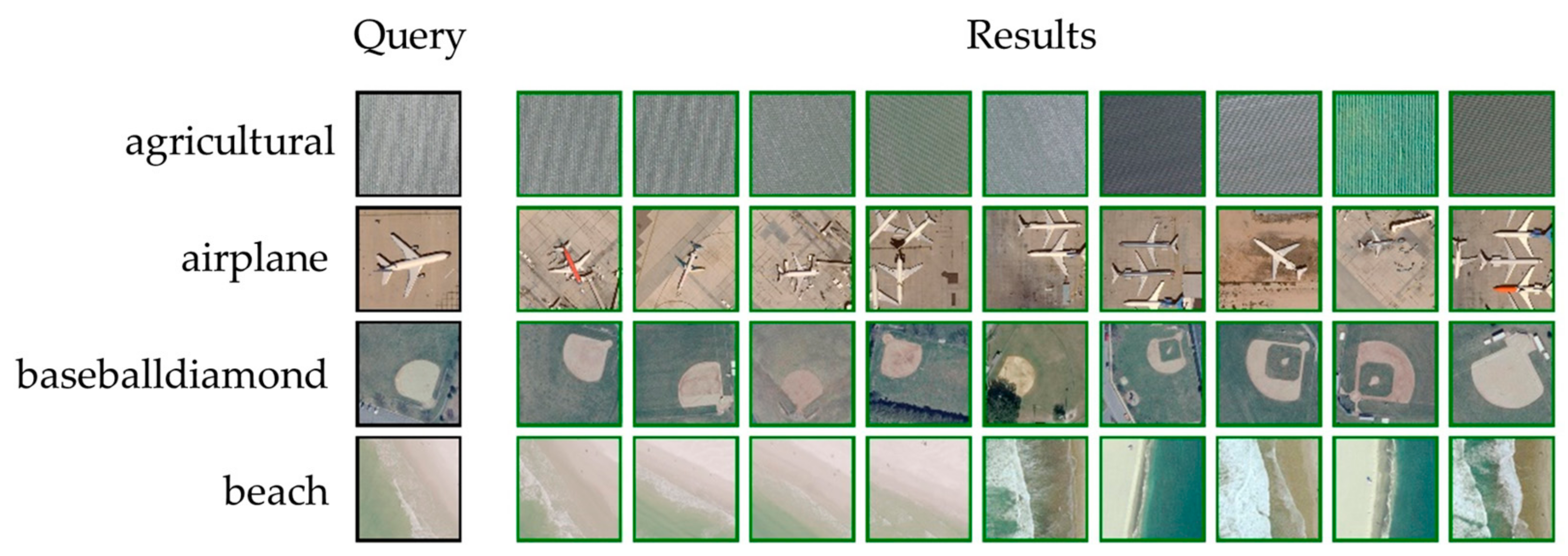
To verify the validity of our proposed method, we compared it with our previous work using the settings mentioned in Section 4.2. We applied the intra-class ranking loss function to the Proxy-Anchor loss and used Recall@K, mAP@K, and R-Precision@R as performance evaluation metrics on the UCMD, AID, NWPU, and Pattern-Net datasets. We compared our proposed method with several popular deep metric learning methods. The comparison results are shown in

Table 9. Recall@K(%), mAP@K, RP@R performance comparison on AID.

Method	AID
	R1	R2	R4	R8	mAP@10	RP@10
Contrastive [28]	91.85	94.20	95.95	97.55	83.75	86.52
Triplet [31]	92.35	94.90	96.25	97.05	88.65	90.39
N-Pair [32]	88.05	92.20	93.95	95.60	80.85	83.76
A-BIER [71]	82.28	90.51	93.55	96.37	70.51	-
DCES [72]	85.39	91.02	95.27	96.63	72.53	-
Circle [73]	93.90	95.15	96.73	97.25	89.40	90.73
MS [33]	92.45	94.70	95.55	96.15	88.40	90.20
SoftTriple [39]	93.45	95.20	96.60	97.30	89.41	90.98
Proxy-NCA [37]	93.35	95.00	96.80	97.30	86.68	89.56
LDM [74]	93.20	94.90	96.00	96.80	89.94	90.95
Proxy-Anchor [40]	93.30	94.90	96.45	97.20	89.80	90.90
Proxy-Anchor+gen	94.30	95.50	96.90	97.70	90.48	91.84

,

Table 10. Recall@K(%), mAP@K, RP@R performance comparison on UCMD.

Method	UCMD
	R1	R2	R4	R8	mAP@10	RP@10
Contrastive [28]	96.19	96.90	98.57	98.80	89.53	90.19
Triplet [31]	97.35	98.09	98.57	98.80	91.45	93.16
N-Pair [32]	94.63	95.23	96.90	98.09	83.97	84.80
A-BIER [71]	86.52	89.96	92.61	94.76	72.11	-
DCES [72]	87.45	91.02	94.27	96.32	78.93	-
Circle [73]	97.90	98.80	99.15	99.30	92.80	93.93
MS [33]	97.20	97.61	98.80	99.28	92.15	93.42
SoftTriple [39]	97.31	98.33	99.18	99.18	91.90	92.54
Proxy-NCA [37]	97.85	98.19	99.04	99.32	89.30	91.30
LDM [74]	97.93	98.67	99.04	99.28	92.65	93.71
Proxy-Anchor [40]	97.77	98.57	98.80	98.80	92.45	93.81
Proxy-Anchor+gen	98.53	99.08	99.27	99.28	93.62	94.80

and

Table 11. Recall@K(%), mAP@K, RP@R performance comparison on NWPU.

Method	NWPU
	R1	R2	R4	R8	mAP@10	RP@10
Contrastive [28]	87.75	92.06	94.66	96.53	83.16	86.95
Triplet [31]	93.33	96.04	97.20	97.82	91.76	93.36
N-Pair [32]	87.80	91.97	94.50	96.36	84.02	87.07
Circle [73]	94.70	96.23	97.35	97.90	93.34	94.49
SoftTriple [39]	95.03	96.80	97.80	97.93	92.40	93.80
MS [33]	94.76	95.96	96.93	97.24	93.95	94.53
Proxy-NCA [37]	94.50	96.54	97.63	97.84	91.49	93.57
LDM [74]	95.06	96.88	97.50	97.96	93.58	94.71
Proxy-Anchor [40]	95.12	96.58	97.54	97.90	93.60	94.60
Proxy-Anchor+gen	95.75	97.12	97.70	98.05	94.45	95.51

. In the table, “MS” stands for “Multi-Similarity” and “LDM” stands for “Learnable Dynamic Margin”. The meaning is the same in the following tables.

It can be found that Proxy-Anchor+gen loss achieves optimal results for the metrics on all three datasets. The results of the comparison experiments validate the effectiveness and superiority of our proposed intra-class ranking loss function. And this indicates that the intra-class ranking loss can learn an embedding space with high discriminability and that the learned embedding space can achieve good class separation while retaining some intra-class differences.

Also, to verify the effectiveness of our proposed intra-class ranking loss with less training data, we used 10% of the PatternNet dataset for training and the remaining 90% for testing, and compared it with other classical loss functions.

As shown in

Table 12. Recall@K(%), mAP@K, RP@R performance comparison on Pattern-Net.

Method	Pattern-Net
	R1	R2	R4	R8	mAP@10	RP@10
Contrastive [28]	97.24	98.45	99.12	99.52	94.59	94.95
Triplet [31]	98.63	99.25	99.51	99.67	97.30	97.71
N-Pair [32]	95.83	97.16	98.15	98.83	92.32	92.87
Circle [73]	98.88	99.47	99.60	99.78	97.63	98.03
SoftTriple [39]	98.70	99.50	99.63	99.79	97.70	98.10
MS [33]	98.52	98.96	99.20	99.41	96.78	97.33
Proxy-NCA [37]	98.45	99.02	99.07	99.28	97.34	97.97
LDM [74]	98.55	99.17	99.25	99.38	97.35	97.95
Proxy-Anchor [40]	98.50	99.03	99.04	99.08	97.51	97.80
Proxy-Anchor+gen	99.10	99.45	99.50	99.70	98.10	98.38

, Proxy-Anchor + intra-class ranking loss achieves the best results on Recall@1, mAP@10, and RP@10 with fewer training samples. It proves that with less training data, the intra-class ranking loss can rely on sample generation to learn more information and use it for feature extraction compared to other losses. This also applies when there are few training samples, since SoftTriple can overcome fine-grained datasets with large intra-class sample differences. Therefore, there are more matching images in the first K (K > 1) retrieval results and Recall@K (K > 1) will outperform the other loss functions.

We conducted experiments by combining intra-class ranking loss with multi-similarity loss, Proxy-NCA loss, and Proxy-Anchor loss on AID and UCMD datasets, respectively. Unlike the dataset partitioning approach mentioned in Section 4.2, we used 80% of the classes in the UCMD and AID datasets for training and the remaining 20% for testing. The results are shown in

Table 13. Recall@K(%), mAP@K, RP@R performance comparison on AID and UCMD.

Method	UCMD						AID
	R1	R2	R4	R8	mAP@10	RP@10	R1	R2	R4	R8	mAP@10	RP@10
MS [33]	96.00	97.50	98.10	98.95	86.70	89.74	91.70	95.70	97.75	98.15	83.84	87.71
MS+gen	97.25	98.35	98.80	99.05	89.38	92.09	92.80	95.75	98.35	99.25	85.97	88.98
Proxy-NCA [37]	96.75	98.00	98.75	99.00	88.68	91.67	92.20	95.70	97.50	98.35	87.16	88.06
Proxy-NCA+gen	97.50	98.25	99.25	99.75	90.78	92.74	93.85	97.00	98.55	99.55	88.73	90.93
Proxy-Anchor [40]	97.00	98.75	99.25	99.75	89.11	91.20	93.45	96.95	98.10	99.20	87.22	89.01
Proxy-Anchor+gen	98.50	99.00	99.25	100.00	91.09	93.20	94.85	97.10	98.80	99.75	89.50	91.29

, with the addition of the intra-class sorting loss, all three metrics of loss show an improvement of about 1% to 2% in the retrieval metrics. The experimental results demonstrate the effectiveness of our proposed intra-class ranking loss. It can help the network better utilize the intra-class differences and make up for the shortcomings of the traditional metric loss function. When the distributions of the training and test sets are different, the intra-class ranking loss can be good at mining intra-class differences and make the network learn more.

We trained the network using one of UCMD and AID as a training set and the other as a testing set [27]. The experimental results are shown in

Table 14. Recall@K(%), mAP@K, RP@R performance comparison on UCMD(training set)–AID(testing set) and AID(training set)–UCMD(testing set).

Method	UCMD(Training Set)– AID (Testing Set)						AID (Training Set)– UCMD (Testing Set)
	R1	R2	R4	R8	mAP@10	RP@10	R1	R2	R4	R8	mAP@10	RP@10
MS [33]	95.73	96.64	97.76	98.29	89.65	90.95	95.80	96.40	97.40	98.80	88.19	90.67
MS+gen	96.70	97.79	98.58	99.10	91.03	92.05	96.40	97.50	98.70	99.10	89.81	91.93
Proxy-NCA [37]	96.14	97.64	98.32	98.58	92.66	93.34	96.20	97.80	98.40	99.00	90.11	92.31
Proxy-NCA+gen	97.61	98.07	99.05	99.26	94.16	94.48	97.90	98.50	99.00	99.30	91.36	93.90
Proxy-Anchor [40]	96.30	97.88	98.29	99.00	92.51	94.04	97.20	97.90	98.70	99.10	90.50	91.37
Proxy-Anchor+gen	97.85	98.10	99.08	99.58	94.19	95.43	98.30	98.70	99.10	99.70	92.42	93.94

, where the retrieval effectiveness of all three metric losses is improved after incorporating intra-class ranking. When the training set and testing set are from different domains, our proposed method can utilize the intra-class differences well in the training set for feature extraction. In addition, it has better performance and improvement in the testing set.

5.3. Visualization

In this section, we show the retrieval results of the trained network on four datasets by visualization. Where the black box represents the query image, the green box represents the successful result and the red box represents the failed result.

We randomly select four query images from the test set for retrieval and returned the top nine images in terms of similarity given by the algorithm. Figure 5 and Figure 6 show that our algorithm has good retrieval performance and correctness.

We use the T-SNE technique to visualize the embedding space and the results are shown in Figure 7. Most of the images on the left are parking lots. Most of the pictures on the upper right are deserts. Most of the pictures on the bottom right are bridges. It can be seen that images of the same class are clustered together in the embedding space.

6. Conclusions

In this paper, we found a problem that traditional metric learning methods in the field of remote sensing image retrieval generally overlook, which is the neglect of intra-class differences while focusing on inter-class differences. However, the intra-class differences are also very helpful for feature extraction in the network. Therefore, we designed a new sample generation mechanism to generate samples from positive samples that meet the boundary constraints, to obtain quantifiable intra-class differences from real positive samples. Based on the sample generation relationship, we used a self-supervised approach to design an intra-class ranking loss function, which improves the discriminability of the generated embedding space for samples of the same class and maintains their ranking relationship in the embedding space. Moreover, this loss function can be easily combined with existing deep metric learning methods. The embedding space obtained through this loss function not only maintains inter-class separability but also distinguishes subtle intra-class differences, thereby providing better global and local structures for retrieval and ranking.

We conducted extensive experiments on four commonly used remote sensing image datasets, using Recall@K, mAP@K, and R-Precision@R as evaluation metrics for image retrieval. The results showed that using the sample-generated intra-class ranking loss function can effectively improve the performance of image retrieval.

References

1. Smeulders, A.W.M.; Worring, M.; Santini, S.; Gupta, A.; Jain, R. Content-based image retrieval at the end of the early years. IEEE Trans. Pattern Anal. Mach. Intell. 2000, 22, 1349–1380. [Google Scholar] [CrossRef]
2. Zheng, L.; Yang, Y.; Tian, Q. SIFT meets CNN: A decade survey of instance retrieval. IEEE Trans. Pattern Anal. Mach. Intell. 2017, 40, 1224–1244. [Google Scholar] [CrossRef] [PubMed] [Green Version]
3. Rui, Y.; Huang, T.S.; Chang, S.-F. Image retrieval: Past, present, and future. J. Vis. Commun. Image Represent. 1999, 10, 39–62. [Google Scholar] [CrossRef]
4. Daschiel, H.; Datcu, M. Information mining in remote sensing image archives: System evaluation. IEEE Trans. Geosci. Remote Sens. 2005, 43, 188–199. [Google Scholar] [CrossRef]
5. Tong, X.-Y.; Xia, G.-S.; Hu, F.; Zhong, Y.; Datcu, M.; Zhang, L. Exploiting Deep Features for Remote Sensing Image Retrieval: A Systematic Investigation. IEEE Trans. Big Data 2020, 6, 507–521. [Google Scholar] [CrossRef] [Green Version]
6. Long, Y.; Zhao, F.; Zheng, M.; Jin, G.; Zhang, H.; Wang, R. A Novel Azimuth Ambiguity Suppression Method for Spaceborne Dual-Channel SAR-GMTI. IEEE Geosci. Remote Sens. Lett. 2021, 18, 87–91. [Google Scholar] [CrossRef]
7. Kim, S.Y.; Myung, N.H.; Kang, M.J. Antenna Mask Design for SAR Performance Optimization. IEEE Geosci. Remote Sens. Lett. 2009, 6, 443–447. [Google Scholar]
8. Kang, M.-S.; Baek, J.-M. Efficient SAR Imaging Integrated with Autofocus via Compressive Sensing. IEEE Geosci. Remote Sens. Lett. 2022, 19, 4514905. [Google Scholar] [CrossRef]
9. Long, Y.; Zhao, F.; Zheng, M.; Jin, G.; Zhang, H. An Azimuth Ambiguity Suppression Method Based on Local Azimuth Ambiguity-to-Signal Ratio Estimation. IEEE Geosci. Remote Sens. Lett. 2020, 17, 2075–2079. [Google Scholar] [CrossRef]
10. Kang, M.-S.; Baek, J.-M. SAR Image Reconstruction via Incremental Imaging with Compressive Sensing. IEEE Trans. Aerosp. Electron. Syst. 2023, 59, 4450–4463. [Google Scholar] [CrossRef]
11. Kim, S.Y.; Myung, N. An optimal antenna pattern synthesis for active phased array SAR based on particle swarm optimization and adaptive weighting factor. Prog. Electromagn. Res. 2009, 10, 129–142. [Google Scholar] [CrossRef] [Green Version]
12. Zheng, J.; Song, X.; Yang, G.; Du, X.; Mei, X.; Yang, X. Remote Sensing Monitoring of Rice and Wheat Canopy Nitrogen: A Review. Remote Sens. 2022, 14, 5712. [Google Scholar] [CrossRef]
13. Sklyar, E.; Rees, G. Assessing Changes in Boreal Vegetation of Kola Peninsula via Large-Scale Land Cover Classification between 1985 and 2021. Remote Sens. 2022, 14, 5616. [Google Scholar] [CrossRef]
14. Jeon, J.; Tomita, T. Investigating the Effects of Super Typhoon HAGIBIS in the Northwest Pacific Ocean Using Multiple Observa-tional Data. Remote Sens. 2022, 14, 5667. [Google Scholar] [CrossRef]
15. Heidari, A.; Jafari Navimipour, N.; Unal, M.; Zhang, G. Machine learning applications in internet-of-drones: Systematic review, recent deployments, and open issues. ACM Comput. Surv. 2023, 55, 1–45. [Google Scholar] [CrossRef]
16. Darbandi, M. Proposing New Intelligence Algorithm for Suggesting Better Services to Cloud Users based on Kalman Filtering. Comput. Sci. Appl. 2017, 5, 11–16. [Google Scholar]
17. Vahdat, S. The role of IT-based technologies on the management of human resources in the COVID-19 era. Kybernetes 2021, 51, 2065–2088. [Google Scholar] [CrossRef]
18. Zadeh, F.A.; Bokov, D.O.; Yasin, G.; Vahdat, S.; Abbasalizad-Farhangi, M. Central obesity accelerates leukocyte telomere length (LTL) shortening in apparently healthy adults: A systematic review and meta-analysis. Crit. Rev. Food Sci. 2023, 63, 2119–2128. [Google Scholar] [CrossRef]
19. Rahhal, M.M.A.; Bencherif, M.A.; Bazi, Y.; Alharbi, A.; Mekhalfi, M.L. Contrasting Dual Transformer Architectures for Multi-Modal Remote Sensing Image Retrieval. Appl. Sci. 2023, 13, 282. [Google Scholar] [CrossRef]
20. Krizhevsky, A.; Sutskever, I.; Hintonm, G.E. Imagenet classification with deep convolutional neural networks. Commun. ACM 2017, 60, 84–90. [Google Scholar] [CrossRef] [Green Version]
21. Musgrave, K.; Belongie, S.; Lim, S.-N. A metric learning reality check. In Proceedings of the European Conference on Computer Vision, Glasgow, UK, 23–28 August 2020; pp. 681–699. [Google Scholar]
22. Zhang, Y.; Zheng, X.; Lu, X. Remote Sensing Image Retrieval by Deep Attention Hashing with Distance-Adaptive Ranking. IEEE J. Sel. Top. Appl. Earth Obs. Remote Sens. 2023, 16, 4301–4311. [Google Scholar] [CrossRef]
23. Guo, J.; Guan, X. Deep Adversarial Cascaded Hashing for Cross-Modal Vessel Image Retrieval. IEEE J. Sel. Top. Appl. Earth Obs. Remote Sens. 2023, 16, 2205–2220. [Google Scholar] [CrossRef]
24. Tan, X.; Zou, Y.; Guo, Z.; Zhou, K.; Yuan, Q. Deep Contrastive Self-Supervised Hashing for Remote Sensing Image Retrieval. Remote Sens. 2022, 14, 3643. [Google Scholar] [CrossRef]
25. Sun, Y.; Ye, Y.; Li, X.; Feng, S.; Zhang, B.; Kang, J.; Dai, K. Unsupervised deep hashing through learning soft pseudo label for remote sensing image retrieval. Knowl.-Based Syst. 2022, 239, 107807. [Google Scholar] [CrossRef]
26. Hou, D.; Wang, S.; Tian, X.; Xing, H. An Attention-Enhanced End-to-End Discriminative Network with Multiscale Feature Learning for Remote Sensing Image Retrieval. IEEE J. Sel. Top. Appl. Earth Obs. Remote sens. 2022, 15, 8245–8255. [Google Scholar] [CrossRef]
27. Hou, D.; Wang, S.; Tian, X.; Xing, H. PCLUDA: A Pseudo-Label Consistency Learning- Based Unsupervised Domain Adaptation Method for Cross-Domain Optical Remote Sensing Image Retrieval. IEEE. Trans. Geosci. Remote. Sens. 2023, 61, 5600314. [Google Scholar] [CrossRef]
28. Bromley, J.; Bentz, J.W.; Bottou, L.; Guyon, I. Signature verification using a “siamese” time delay neural network. Int. J. Pattern Recogn. 1993, 7, 669–688. [Google Scholar] [CrossRef] [Green Version]
29. Schroff, F.; Kalenichenko, D.; Philbin, J. Facenet: A unified embedding for face recognition and clustering. In Proceedings of the Proceedings of the IEEE Conference on Computer Vision and Pattern Recognition, Boston, MA, USA, 7–12 June 2015; pp. 815–823.
30. Wang, J.; Song, Y.; Leung, T.; Rosenberg, C.; Wang, J.; Philbin, J.; Chen, B.; Wu, Y. Learning fine-grained image similarity with deep ranking. In Proceedings of the IEEE Conference on Computer Vision and Pattern Recognition, Columbus, OH, USA, 23–28 June 2014; pp. 1386–1393. [Google Scholar]
31. Hoffer, E.; Ailon, N. Deep metric learning using triplet network. In Similarity-Based Pattern Recognition, Proceedings of the Third International Workshop, SIMBAD 2015, Copenhagen, Denmark, 12–14 October 2015; Lecture Notes in Computer Science (IncludingSubseries Lecture Notes in Artificial Intelligence and Lecture Notes in Bioinformatics); Springer: Cham, Switzerland, 2015; Volume 9370, pp. 84–92. [Google Scholar]
32. Sohn, K. Improved deep metric learning with multi-class n-pair loss objective. In Proceedings of the Advances in Neural Information Processing Systems, Barcelona, Spain, 5–10 December 2016; pp. 1857–1865. [Google Scholar]
33. Wang, X.; Han, X.; Huang, W.; Dong, D.; Scott, M.R. Multi-similarity loss with general pair weighting for deep metric learning. In Proceedings of the IEEE/CVF Conference on Computer Vision and Pattern Recognition, Long Beach, CA, USA, 15–20 June 2019; pp. 5017–5025. [Google Scholar]
34. Wu, C.-Y.; Manmatha, R.; Smola, A.J.; Krähenbühl, P. Sampling matters in deep embedding learning. In Proceedings of the IEEE International Conference on Computer Vision, Venice, Italy, 22–29 October 2017; pp. 2859–2867. [Google Scholar]
35. Harwood, B.; Kumar, V.; Carneiro, G.; Reid, I.; Drummond, T. Smart mining for deep metric learning. In Proceedings of the IEEE International Conference on Computer Vision, Venice, Italy, 22–29 October 2017; pp. 2840–2848. [Google Scholar]
36. Gajić, B.; Amato, A.; Gatta, C. Fast hard negative mining for deep metric learning. Pattern Recogn. 2021, 112, 107795. [Google Scholar] [CrossRef]
37. Movshovitz-Attias, Y.; Toshev, A.; Leung, T.K.; Loffe, S.; Singh, S. No fuss distance metric learning using proxies. In Proceedings of the IEEE International Conference on Computer Vision, Venice, Italy, 22–29 October 2017; pp. 360–368. [Google Scholar]
38. The, E.W.; Devries, T.; Taylor, G.W. Proxynca++: Revisiting and Revitalizing Proxy Neighborhood Component Analysis. In Proceedings of the Computer Vision–ECCV 2020: Glasgow, Scotland, UK, 23–28 August 2020; pp. 448–464. [Google Scholar]
39. Qian, Q.; Shang, L.; Sun, B.; Hu, J.; Tacoma, T.; Li, H.; Jin, R. Softtriple loss: Deep metric learning without triplet sampling. In Proceedings of the IEEE/CVF International Conference on Computer Vision, Seoul, Republic of Korea, 27 October–2 November 2019; pp. 6449–6457. [Google Scholar]
40. Kim, S.; Kim, D.; Cho, M.; Kwak, S. Proxy anchor loss for deep metric learning. In Proceedings of the IEEE/CVF Conference on Computer Vision and Pattern Recognition, Seattle, WA, USA, 13–19 June 2020; pp. 3235–3244. [Google Scholar]
41. Kan, S.; He, Z.; Cen, Y.; Li, Y.; Mladenovic, V.; He, Z. Contrastive Bayesian Analysis for Deep Metric Learning. IEEE Trans. Pattern Anal. Mach. Intell. 2023, 45, 7220–7238. [Google Scholar] [CrossRef]
42. Jin, Y.; Lu, H.; Zhu, W.; Huo, W. Deep learning based classification of multi-label chest X-ray images via dual-weighted metric loss. Comput. Biol. Med. 2023, 157, 106683. [Google Scholar] [CrossRef]
43. Saeki, S.; Kawahara, M.; Aman, H. Multi proxy anchor family loss for several types of gradients. Comput. Vis. Image Underst. 2023, 229, 103654. [Google Scholar] [CrossRef]
44. Wang, X.; Hua, Y.; Kodirov, E.; Robertson, N.M. Ranked List Loss for Deep Metric Learning. IEEE Trans. Pattern Anal. Mach. Intell. 2022, 44, 5414–5429. [Google Scholar]
45. Ko, B.; Gu, G. Embedding expansion: Augmentation in embedding space for deep metric learning. In Proceedings of the IEEE/CVF Conference on Computer Vision and Pattern Recognition, Seattle, WA, USA, 14–19 June 2020; pp. 7253–7262. [Google Scholar]
46. Duan, Y.; Lu, J.; Zheng, W.; Zhou, J. Deep adversarial metric learning. IEEE. Trans. Image Process. 2019, 29, 2037–2051. [Google Scholar] [CrossRef]
47. Lin, X.; Duan, Y.; Dong, Q.; Lu, J.; Zhou, J. Deep variational metric learning. In Proceedings of the European Conference on Computer Vision (ECCV), Munich, Germany, 8–14 September 2018; pp. 714–729. [Google Scholar]
48. Zhao, Y.; Jin, Z.; Qi, G.-J.; Lu, H.; Hua, X.-S. An adversarial approach to hard triplet generation. In Proceedings of the European Conference on Computer Vision (ECCV), Munich, Germany, 8–14 September 2018; pp. 508–524. [Google Scholar]
49. Zheng, W.; Chen, Z.; Lu, J.; Zhou, J. Hardness-aware deep metric learning. IEEE. Trans. Pattern Anal. Mach. Intell. 2019, 34, 3214–3228. [Google Scholar]
50. Gu, G.; Ko, B. Symmetrical synthesis for deep metric learning. In Proceedings of the AAAI Conference on Artificial Intelligence, New York, NY, USA, 7–12 February 2020; pp. 10853–10860. [Google Scholar]
51. Gu, G.; Ko, B.; Kim, H.-G. Proxy synthesis: Learning with synthetic classes for deep metric learning. In Proceedings of the AAAI Conference on Artificial Intelligence, Virtual, 2–9 February 2021; pp. 1460–1468. [Google Scholar]
52. He, K.; Fan, H.; Wu, Y.; Xie, S.; Girshick, R. Momentum contrast for unsupervised visual representation learning. In Proceedings of the IEEE/CVF Conference on Computer Vision and Pattern Recognition, Seattle, WA, USA, 13–19 June 2020; pp. 9726–9735. [Google Scholar]
53. Pathak, D.; Krahenbuhl, P.; Donahue, J.; Darrell, T.; Efros, A.A. Context encoders: Feature learning by inpainting. In Proceedings of the IEEE Conference on Computer Vision and Pattern Recognition, Las Vegas, NV, USA, 27–30 June 2016; pp. 2536–2544. [Google Scholar]
54. Gidaris, S.; Singh, P.; Komodakis, N. Unsupervised representation learning by predicting image rotations. In Proceedings of the International Conference on Learning Representations Vancouver Convention Center, Vancouver, BC, Canada, 30 April–3 May 2018. [Google Scholar]
55. Zhai, X.; Oliver, A.; Kolesnikov, A.; Beyer, L. S4L: Self-supervised semi-supervised learning. In Proceedings of the IEEE/CVF International Conference on Computer Vision, Seoul, Republic of Korea, 27 October–2 November 2019; pp. 1476–1485. [Google Scholar]
56. Roth, K.; Brattoli, B.; Ommer, B. Mic: Mining interclass characteristics for improved metric learning. In Proceedings of the IEEE/CVF International Conference on Computer Vision, Seoul, Republic of Korea, 27 October–2 November 2019; pp. 7999–8008. [Google Scholar]
57. Wang, X.; Zhang, H.; Huang, W.; Scott, M.R. Cross-batch memory for embedding learning. In Proceedings of the IEEE/CVF Conference on Computer Vision and Pattern Recognition, Seattle, WA, USA, 13–19 June 2020; pp. 6387–6396. [Google Scholar]
58. Zhu, H.; Xu, H.; Ma, X.; Bian, M. Facial Expression Recognition Using Dual Path Feature Fusion and Stacked Attention. Future Intern. 2022, 14, 258. [Google Scholar] [CrossRef]
59. Lu, X.; Ding, W.; Li, H.; Yu, P.; Gu, J. Fine-grained image classification algorithm based on Attention Self-supervision. In Proceedings of the 2021 IEEE 5th Advanced Information Technology, Electronic and Automation Control Conference (IAEAC), Chongqing, China, 12–14 March 2021; pp. 517–521. [Google Scholar]
60. Zhang, X.; Liu, Y.; Huo, C.; Xu, N.; Wang, L.; Pan, C. PSNet: Perspective-sensitive convolutional network for object detection. Neurocomputing 2022, 468, 384–395. [Google Scholar] [CrossRef]
61. Zhang, T.; Yang, L.; Gut, X.; Wang, Y. A Task-Specific Meta-Learning Framework for Few-Shot Sound Event Detection. In Proceedings of the 2022 IEEE 24th International Workshop on Multimedia Signal Processing (MMSP), Shanghai, China, 26–28 September 2022; pp. 1–6. [Google Scholar]
62. Alipour, N.; Tarkhaneh, O.; Awrangjeb, M.; Tian, H. Flower Image Classification Using Deep Convolutional Neural Network. In Proceedings of the 2021 7th International Conference on Web Research (ICWR), Tehran, Iran, 19–20 May 2021; pp. 1–4. [Google Scholar]
63. Zhang, Z.; Zhang, T.; Liu, Z.; Zhang, P.; Tu, S.; Li, Y.; Waqas, M. Fine-grained Ship Image Recognition Based on BCNN with Inception and AM-Softmax. Comput. Mater. Contin. 2022, 73, 1527–1539. [Google Scholar]
64. Fu, Z.; Mao, Z.; Yan, C.; Liu, A.-A.; Xie, H.; Zhang, Y. Self-supervised Synthesis Ranking for Deep Metric Learning. IEEE Trans. Circuits Syst. Video Technol. 2021, 32, 4736–4750. [Google Scholar] [CrossRef]
65. Yang, Y.; Newsam, S. Bag-of-visual-words and spatial extensions for land-use classification. In Proceedings of the 18th SIGSPA-TIAL International Conference on Advances in Geographic Information Systems, San Jose, CA, USA, 2–5 November 2010; pp. 270–279. [Google Scholar]
66. Xia, G.-S.; Hu, J.; Hu, F.; Shi, B.; Bai, X.; Zhong, Y.; Zhang, L.; Lu, X. AID: A benchmark data set for performance evaluation of aerial scene classification. IEEE Trans. Geosci. Remote Sens. 2017, 55, 3965–3981. [Google Scholar]
67. Cheng, G.; Han, J.; Lu, X. Remote sensing image scene classification: Benchmark and state of the art. Proc. IEEE 2017, 105, 1865–1883. [Google Scholar] [CrossRef]
68. Zhou, W.; Newsam, S.; Li, C.; Shao, Z. PatternNet: A benchmark dataset for performance evaluation of remote sensing image retrieval. ISPRS J. Photogramm. Remote Sens. 2018, 145, 197–209. [Google Scholar] [CrossRef] [Green Version]
69. Ioffe, S.; Szegedy, C. Batch Normalization: Accelerating Deep Network Training by Reducing Internal Covariate Shift. In Proceedings of the International Conference on Machine Learning, Lille, France, 6–11 July 2015; pp. 448–456. [Google Scholar]
70. Deng, J.; Dong, W.; Socher, R.; Li, L.-J.; Li, K.; Li, F.-F. Imagenet: A large-scale hierarchical image database. In Proceedings of the 2009 IEEE Conference on Computer Vision and Pattern Recognition, Miami, FL, USA, 20–25 June 2009; pp. 248–255. [Google Scholar]
71. Opitz, M.; Waltner, G.; Possegger, H.; Bischof, H. Deep Metric Learning with BIER: Boosting Independent Embeddings Robustly. IEEE Trans. Pattern Anal. Mach. Intell. 2020, 42, 276–290. [Google Scholar] [CrossRef] [PubMed] [Green Version]
72. Sanakoyeu, A.; Tschernezki, V.; Büchler, U.; Ommer, B. Divide and Conquer the Embedding Space for Metric Learning. In Proceedings of the 2019 IEEE/CVF Conference on Computer Vision and Pattern Recognition (CVPR), Miami, FL, USA, 20–25 June 2019; pp. 471–480. [Google Scholar]
73. Sun, Y.; Cheng, C.; Zhang, Y.; Zhang, C.; Zheng, L.; Wang, Z.; Wei, Y. Circle loss: A unified perspective of pair similarity optimization. In Proceedings of the IEEE/CVF Conference on Computer Vision and Pattern Recognition, Seattle, WA, USA, 13–19 June 2020; pp. 6397–6406. [Google Scholar]
74. Wang, Y.; Liu, P.; Lang, Y.; Zhou, Q.; Shan, X. Learnable dynamic margin in deep metric learning. Pattern Recognit. 2022, 132, 108961. [Google Scholar] [CrossRef]
Figure 1. The framework of deep metric-learning training and retrieval. The above part illustrates the process of how to use deep metric learning for network training and image retrieval in remote-sensing image retrieval tasks. The training phase uses a backbone network for feature extraction to obtain the embedding vectors of the images, and uses a loss function to reverse update the backbone network parameters. The image retrieval phase uses the trained backbone network to generate embedding vectors for each image and returns a number of images similar to the query image by calculating the similarity of these vectors.
Remotesensing 15 03943 g001
Figure 2. The figure illustrates whether differences in intra-class ranking are taken into account. In the figure, Sn denotes the similarity between the positive sample n and the anchor point. If intra-class ranking is not considered, the similarities after training between all positive samples and the anchor point are equal. However, when intra-class ranking is considered, there is a ranking relationship between the similarity of different positive samples and the anchor point in the final learned embedding space.
Remotesensing 15 03943 g002
Figure 3. Sample generation. In the figure, e x represents the embedding vector of the original positive sample a x , r represents a fixed length, and generates samples with ranking relationships by taking different values of n. g x n   represents the embedding vector of the nth generated sample of the original positive sample e x . u n represents a unit vector with direction which is randomly generated before training and obeys a normal distribution, n = 0 , 1 , , N .
Remotesensing 15 03943 g003
Figure 4. A training framework using the intra-class ranking loss function based on sample generation.
Remotesensing 15 03943 g004
Figure 5. Example of AID retrieval results. Column 1 is the query image and columns 2 through 10 are the returned results.
Remotesensing 15 03943 g005
Figure 6. Example of UCMD retrieval results. Column 1 is the query image and columns 2 through 10 are the returned results.
Remotesensing 15 03943 g006
Figure 7. Visualization of the embedding space obtained using our method on the AID dataset.
Remotesensing 15 03943 g007