Article

Study on the Spatial and Temporal Distribution of Urban Vegetation Phenology by Local Climate Zone and Urban–Rural Gradient Approach

1
Remote Sensing Information and Digital Earth Center, College of Computer Science and Technology, Qingdao University, Qingdao 266071, China
2
Key Laboratory of Digital Earth Science, Aerospace Information Research Institute, Chinese Academy of Sciences, Beijing 100094, China
*
Author to whom correspondence should be addressed.
Remote Sens. 2023, 15(16), 3957; https://doi.org/10.3390/rs15163957
Submission received: 10 July 2023 / Revised: 31 July 2023 / Accepted: 4 August 2023 / Published: 10 August 2023
(This article belongs to the Special Issue Remote Sensing for Land Use and Vegetation Mapping)

Abstract

:
Understanding variations in the temporal and spatial distribution of vegetation phenology is essential for adapting to and mitigating future climate change and urbanization. However, there have been limited vegetation phenology studies within small-scale areas such as urban environments over the past decades. Therefore, the present study focuses on Jinan city, Shandong Province, China as the study area and employs a more refined local climate zone (LCZ) approach to investigate spatial and temporal variations in vegetation phenology. The three phenological indicators used in this study from 2007 to 2018, namely, the start of growing season (SOS), the end of growing season (EOS), and the length of growing season (LOS), were provided by MODIS satellite data. The SOS, EOS, and LOS were superimposed on the LCZ and urban–rural gradient to analyze the changes in vegetation phenology, and the applicability of these two analysis methods in the study of urban vegetation phenology was compared by the honest significant difference test. We found that the SOS, EOS, and LOS of vegetation in the study area generally showed an advance, delay, and extension trend, respectively. The means of the SOS and EOS along different LCZ types varied noticeably more than those along urban–rural gradients. In 2016, 77.5%, 80.0%, and 75.8% of LCZ pairs indicated statistically significant differences for SOS, EOS, and LOS, respectively. This study provides a new perspective for the study of urban vegetation phenology which can help in management of urban-scale environments, identification of areas rich in biodiversity, and conservation and restoration of biodiversity in urban areas.

1. Introduction

Phenology has been extensively investigated across various disciplines, including biology, meteorology, agriculture, horticulture, tourism, and more [1]. Vegetation phenology is specifically associated with vegetation growth [2] and other seasonal changes related to cyclical phenomena [3,4,5]. Vegetation phenology is a function of ecosystems, and responds to energy exchange, carbon cycling, and nutrient cycling in terrestrial environments [6,7]. Through the examination of vegetation phenology, it is possible to analyze ecological impacts on terrestrial ecosystems such as biodiversity, carbon emissions, nutrient cycling, land use, and land cover [8]. In recent years, with in-depth research on global change the exploration of vegetation phenology has garnered considerable attention from scholars worldwide [8,9].
In the past two decades China has experienced rapid urbanization, resulting in an increasingly aggravated heat island effect [10,11,12]. The urban heat island (UHI) effect directly manifests as climate warming caused by human activities. Urban environments are complex large-scale systems, and urban vegetation phenology is predominantly influenced by urbanization and climate change [13]. Urban greening initiatives play a role in mitigating the UHI effect, although they impact urban phenology as well. The interaction between the UHI effect and climate change adds complexity to the urban vegetation phenological response mechanism [11]. Urbanization imparts unique local climate characteristics to urban areas [14]. In 2012, Stewart and Oke proposed the concept of a local climate zone (LCZ) [15], a novel land cover classification system aimed at studying the UHI effect. LCZ represents the first standardized approach worldwide for urban climate research, and has become an international benchmark for analyzing urban form and the UHI effect [14]. Within the contexts of global warming and urbanization, more studies have begun focusing on changes in vegetation phenology within urban settings [8,12,16,17,18].
Vegetation information extraction serves as the foundation of vegetation phenology research [19]. The Google Earth Engine platform provides convenient access to a wealth of remote sensing data [19,20,21]. Various factors affect vegetation growth, with climate change and urbanization exerting strong impacts on vegetation growth in urban environments [13]. Numerous scholars have conducted extensive research on the relationship between vegetation phenology and climate change [22]. Multiple studies have examined the spatial and temporal dynamics of vegetation phenology at large regional scales [23,24,25,26]. As urbanization has accelerated, land use and land cover have changed, as has the earth’s surface temperature. The UHI effect can impact the health of residents and the sustainable development of urban areas. Prior to the introduction of the LCZ concept, no standardized criterion existed for comparing the UHI intensity. LCZ is a new land cover classification system for the study of the UHI effect that considers the three-dimensional structural characteristics of buildings, enabling more detailed classification of urban areas and their surroundings [15]. Subsequently, LCZ has gradually emerged as a guiding principle in the field of urban climatology research. After the advent of the LCZ classification system, many researchers began to conduct extensive research into different ways of obtaining LCZ classification data. The methods of LCZ mapping are mainly divided into GIS data-based mapping [27,28] and remote sensing image-based mapping [29,30]. Among them, the mapping method based on remote sensing images is more widely used, mainly including the WUDAPT method and machine learning methods. The World Urban Database and Access Portal Tools (WUDAPT) method is currently the mainstream method [14,31,32,33,34,35].
Urbanization has a profound impact on vegetation phenology, encompassing both urban areas and adjacent rural areas [8,12,36,37,38]. There are discernible differences in the start of growing season (SOS), the end of growing season (EOS), and length of growing season (LOS) between urban and rural areas [8,12,17,37]. The influence of urban climate on vegetation phenology is associated with the distance from the urban center, generally resulting in a longer LOS in urban areas compared to suburban areas [39,40]. Ullah et al. (2020) investigated the effects of urban expansion on vegetation phenology and land surface temperature (LST) in Xi’an. Their results demonstrated that urban area expansion led to a rise in LST and a reduction in vegetation cover. In summary, vegetation and urban greening were found to alleviate the negative effects of urbanization in Xi’an City [41]. In addition, Li et al. (2021) incorporated night light and chlorophyll fluorescence data to analyze vegetation phenological changes and reactions to urbanization in the Dongting Lake Basin [42]. Other studies have conducted spatial and temporal analyses of vegetation phenology based on the UHI effect in urban areas such as Wuhan, Boston, and the suburbs of Milton, Ontario, Canada [43,44,45]. However, significant gaps remain in the study of the effects of urbanization on phenology. To address this gap, Qiu et al. (2017) focused on the transition zone from urban to rural landscapes as the core and analyzed changes in vegetation phenology along this transition zone in Shanghai [18]. Additionally, other scholars have analyzed the disparity between urban and rural phenological indexes by dividing the gradient of Hangzhou phenological data and LST data, revealing a negative relationship among LST and SOS in the spring [12]. Notably, temperature exerts a considerable influence on SOS, while precipitation demonstrates a strong influence on EOS [39]. Furthermore, studies have explored the link between LCZ and LST [46,47,48]. Such analyses play a fundamental role in developing a series of urban planning measures aimed at mitigating the UHI effect.
Urbanization has an impact on the health of people with pollen allergies, as well as on the carbon cycle [9]. Currently, there is considerable interest among scholars from various nations in the phenological changes resulting from alterations in natural environments. However, research on phenological changes induced by urbanization remains relatively limited, with most focusing on urban–rural comparisons while overlooking the dynamics of vegetation phenology in transitional zones [9,19]. In the process of urbanization, diverse combinations of architectural landscapes create distinctive microclimates within urban areas. These microclimate variations contribute to variations in SOS, EOS, and LOS within the urban context [19]. In this study, the LCZ classification system was combined with long-term satellite remote sensing data series and applied to vegetation phenology research in Jinan City in order to explore the advantages of the LCZ classification system in the study of urban vegetation phenology. In general, the main objectives of this paper are: (1) to analyze the spatial and temporal trend change of vegetation phenology in Jinan City during 2007–2018; (2) to explore vegetation phenological changes along the urban–rural gradient (URG) and LCZ types in the study area; and (3) to investigate the applicability of the LCZ classification system for the study of vegetation phenology in an urban region.

2. Materials and Methods
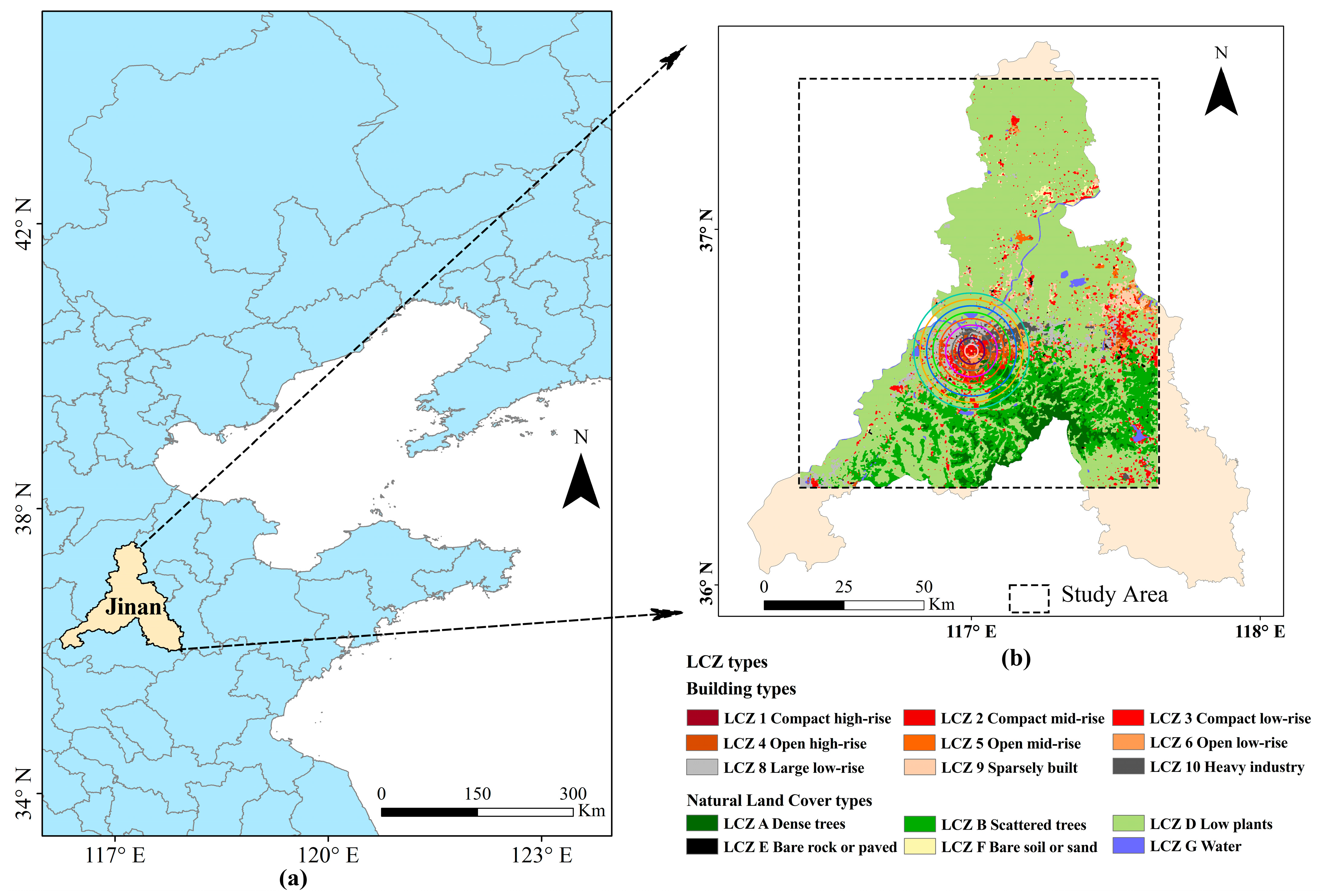
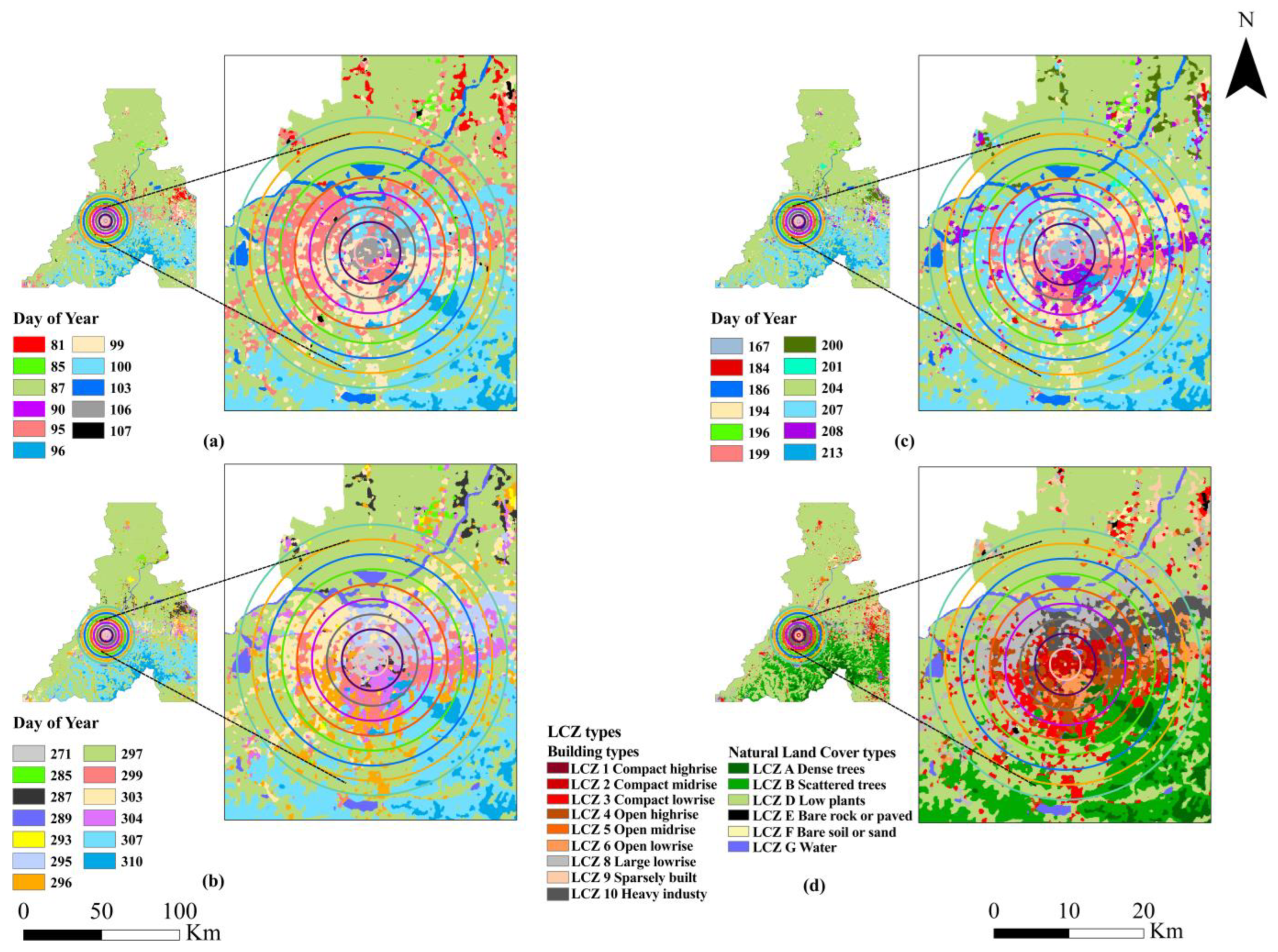
2.1. Study Area

Located in the middle of Shandong province, Jinan City has a total area of 10,244.45 km2 (Figure 1). It is the central city of the Yellow River basin, with Mount Tai to the south and the Yellow River to the north. It is at the junction of low hills and alluvial plains in Shandong, with a higher elevation in the south compared to the northern part. Jinan belongs to the warm temperate continental monsoon climate zone, with monsoons, distinct seasons and adequate light [49,50]. The yearly average temperature is 13.5–15.5 °C and the mean annual precipitation is 600–900 mm [51]. Jinan is the capital of Shandong Province, a large economic and cultural powerhouse on China’s eastern coast. In 2021, the city had a permanent residential population of 9.2 million and an urbanization rate of 75.2% [52]. Rapid urbanization has brought about dramatic changes in land cover from natural landscapes to built areas. As in other large cities, Jinan has been confronted with ecological and environmental problems, including the UHI effect and biodiversity reduction in the context of rapid urbanization. Due to the publicly available LCZ data used in this paper being limited, the study area consists of the rectangular region in Figure 1b.

2.2. Data Sources and Processing

In this study, the LCZ classifies land surfaces in Jinan into 15 types based on different building densities, geometric forms, and surface features [15]. The classification system of LCZ consists of two types: building types and natural land cover types (See Figure 1b). LCZ 1–3 are characterized by compact buildings and little green space. LCZ 4–6 are characterized by having more green space than LCZ 1–3, with less density of buildings. LCZ 9–10 include the remaining city categories. LCZ A–G are all natural land cover types except for LCZ E, which contains paved cover. The WUDAPT provided the LCZ classification data on Jinan City (https://wudapt.cs.purdue.edu/ (accessed on 25 November 2022)). The LCZ classification map of the study area in 2016 was provided by WUDAPT (www.wudapt.org/cities/raw-training-area-download/ (accessed on 25 November 2022)).
The remote sensing dataset used in this study was the MODIS global land cover product MCD12Q2; it uses EVI as the data source, with a spatial resolution of 500 m and a yearly temporal resolution [53]. These data have been validated by in-field observations and applied extensively in phenological studies in small-scale areas, including urban areas [12,39,40,54]. The vegetation phenology data for Jinan were obtained from the Google Earth Engine (https://developers.google.com/earth-engine/datasets/catalog/MODIS_061_MCD12Q2 (accessed on 7 December 2022)). The extracted SOS, EOS, and LOS information were used to characterize vegetation phenology [8,9,55].

2.3. Method

2.3.1. Extraction of Vegetation Phenology Indicators

First, the EVI time series data were preprocessed to reduce the effects of clouds, aerosols, snow, and observation angles. Then, a sliding window approach (five consecutive phase EVI values) was utilized to identify continuous increasing or decreasing intervals. When the maximum value and amplitude of an interval met the given threshold conditions, it was identified as a growth cycle process. For each growth cycle, a segmented logistic function was fitted, and the inflection points of its curvature value changes were used to determine the greenup, midgreenup, maturity, peak, senescence, midgreendown, and dormancy. Greenup and dormancy of MCD12Q2 were extracted to characterize SOS and EOS, respectively. Then, the raster images were converted to the date of the year, with the raster values representing the number of days until 1 January 1970. Meanwhile, several outliers were excluded. Total values greater than day 180 and less than day 30 in SOS and values greater than day 350 and less than day 240 in EOS were removed [8]. Among these, the LOS was obtained by referring to the difference between EOS and SOS.

2.3.2. Trend Analysis of Phenological Indicators

The trend slope S of SOS, EOS, and LOS from 2007 to 2018 was calculated using the simple linear regression analysis method in ArcGIS software; S was calculated using the least squares method as follows:
S = n × i = 1 n i × P i i = 1 n i i = 1 n P i n × i = 1 n i 2 i = 1 n i 2
where n = 12, i is the year number, Pi is the phenological parameter of the year i, S is the slope of the univariate linear regression equation, and S > 0 indicates that the overall trend of phenological parameters in these 12 years is delayed (prolonged) (otherwise, it is advanced (shortened)).

2.3.3. The URGs Division Based on LCZs and Phenological Indicators

The geometric center point of the LCZ1 area was obtained using ArcGIS software, and was used as the city’s center. The starting point for the division of the URG and the study area was divided into ten gradients with a radial gradient of 2 km (referred to as 2 km), with gradients of 2 km, 4 km, 6 km, 8 km, 10 km, 12 km, 14 km, 16 km, 18 km, and 18 km+ (i.e., areas other than the maximum circular area of the study area). This division refers to the division of the Austin metropolitan area [55]. The geometric center point obtained by the above method was used as the starting point for dividing phenological indicators, and the phenological indicators were divided by the same URG.

2.3.4. Analysis of Phenological Indexes Based on LCZs and URGs

The obtained phenological indexes were overlaid on LCZs and URGs for statistical analysis. A Python program was used to visualize SOS, EOS, and LOS from 2007–2018 for different URGs and LCZs, respectively. First, one-way ANOVA was employed to determine the vegetation phenology change between different LCZs and URGs. Second, the honest significant difference (HSD) test was used to assess the SOS, EOS, and LOS difference between different LCZ pairs and URG pairs [55]. The HSD test, which compares all pairs of averages simultaneously, has been widely used [56]. The value of the HSD test was obtained by taking the absolute value of the difference between paired means and then dividing it by the standard error of the average determined by the one-way ANOVA test. With the HSD test, a single value was calculated to compare the differences between all pairs of means. This value was called HSD, provided by the following formula:
H S D = q α ,   k ,   n k M S E n j
where q is significance level α, k is the mean in the test, and nk is the error freedom. Any difference between the mean values of any pair that exceeds the HSD value indicates that the difference between the mean pairs is significant. The mean of SOS, EOS, and LOS on each LCZ category was obtained. The absolute value of the difference between their averages was calculated, the significance level α was set, and the HSD value was found to determine which mean values did not exceed the HSD. The phenological mean for these categories was not significant. The same calculation method was applied to phenological indicators overlaid on URGs.

3. Results

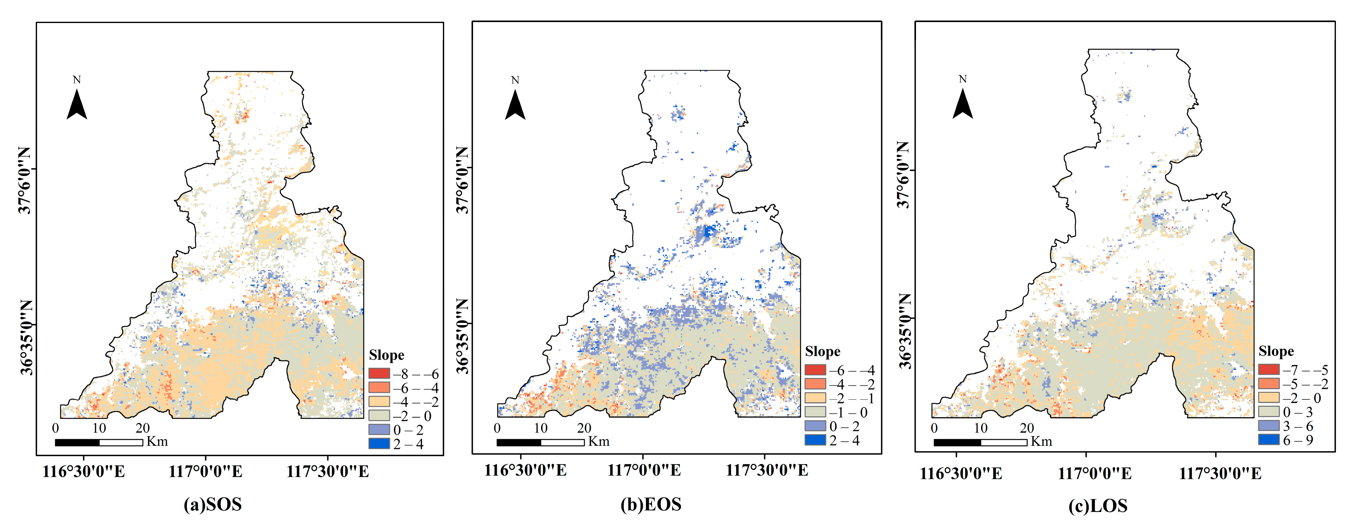
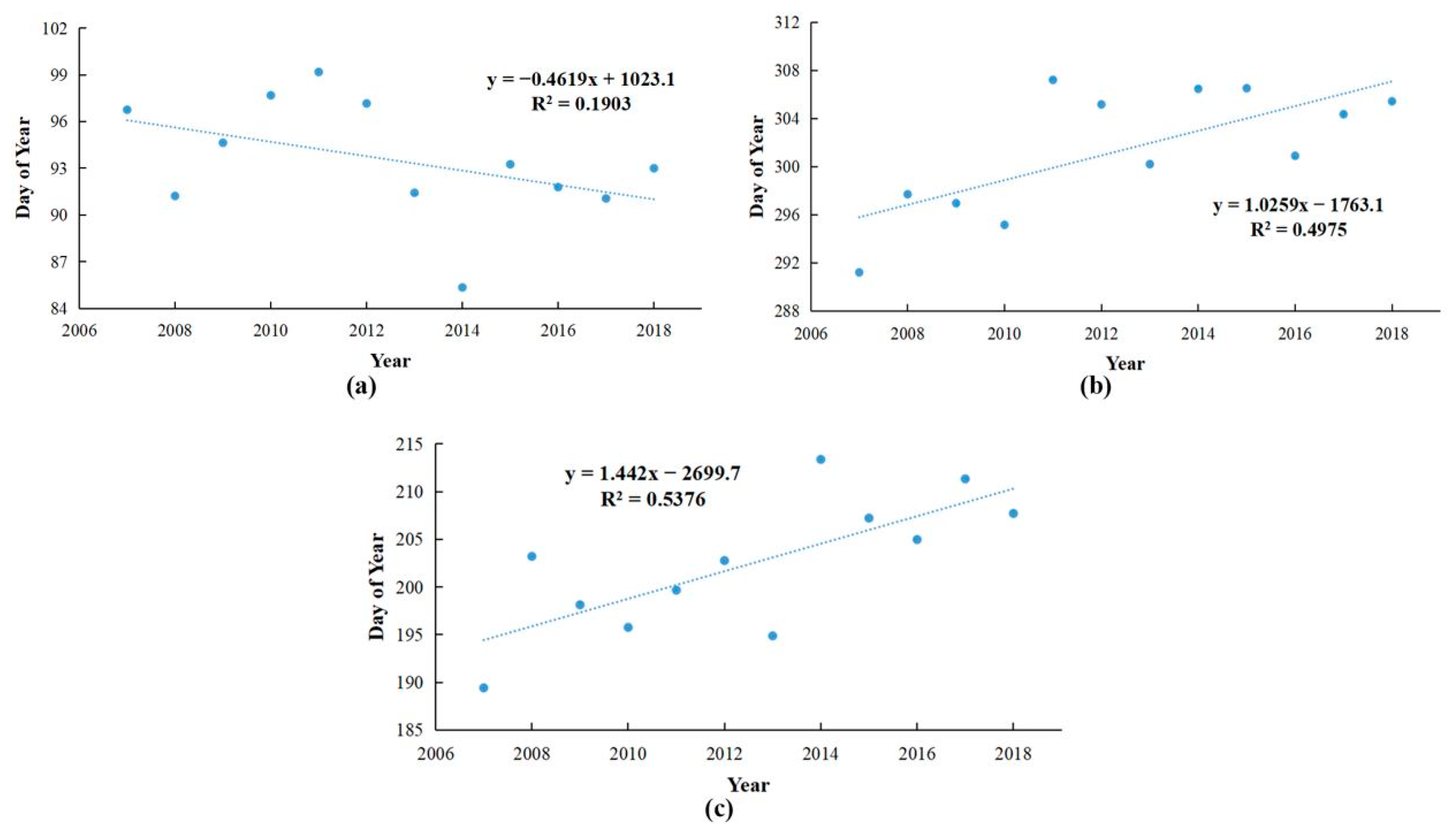
3.1. Spatio-Temporal Distribution of Vegetation Phenology over Jinan City

Figure 2 showed the spatial distribution of vegetation phenology in Jinan between 2007 to 2018. From the north to south of Jinan City, the SOS and EOS showed a gradual delay. Most of the SOS in the north occurred around 80–90 days; in 2013 it was even earlier than 80 days. In the southern region, it was mostly concentrated around 90–110 days, and in 2010 and 2011 it was even around 120 days. For the EOS, it was focused on 300–320 days in the south of Jinan and 280–300 days in the northern areas. Since 2014 it has been clustered in the range of 200–220 days, and even 240–260 days in the north. In general, from 2007 to 2018 the SOS, EOS, and LOS showed a large area of advance, delay, and extension, respectively (see Figure 3). The delay of the EOS was most pronounced in the central region of Jinan.
Figure 4 illustrates the interannual variation of vegetation phenology in Jinan from 2007–2018. During the study period, SOS, EOS, and LOS showed a trend of advance, delay, and extension, respectively. Figure 4a shows that the SOS was on average 0.46d·(10a)−1 earlier. The average SOS for these 12 years was day 93, with a range of days of 85–99. Figure 4b demonstrated the average EOS delay of 10.3d·(10a)−1. The average EOS during the study period was day 301, and the fluctuation range was days 291–307. The LOS lengthened by an average of 14.4d·(10a)−1. The average LOS for 12 years was day 202, with a fluctuation range of days 189–213 (Figure 4c).

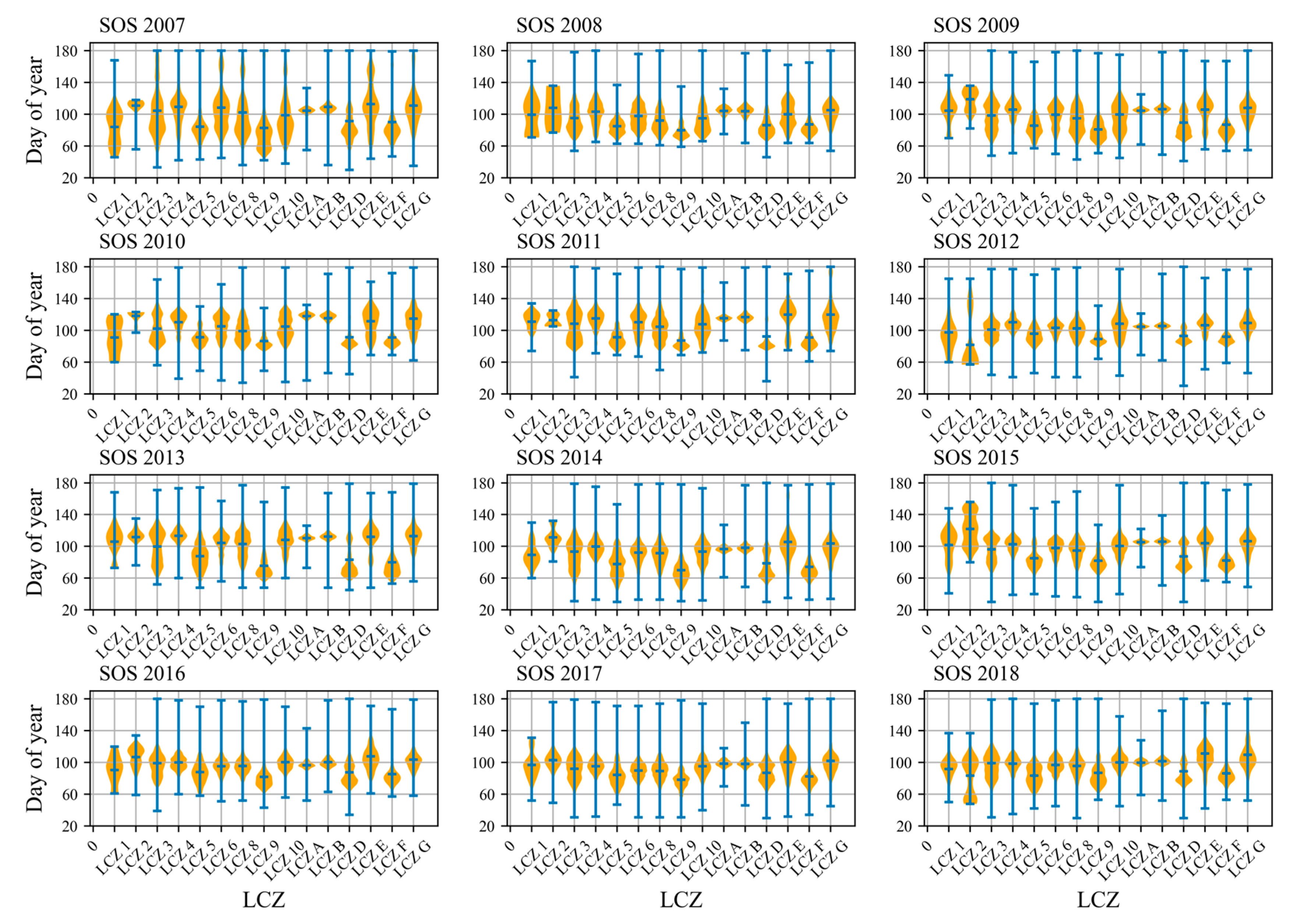
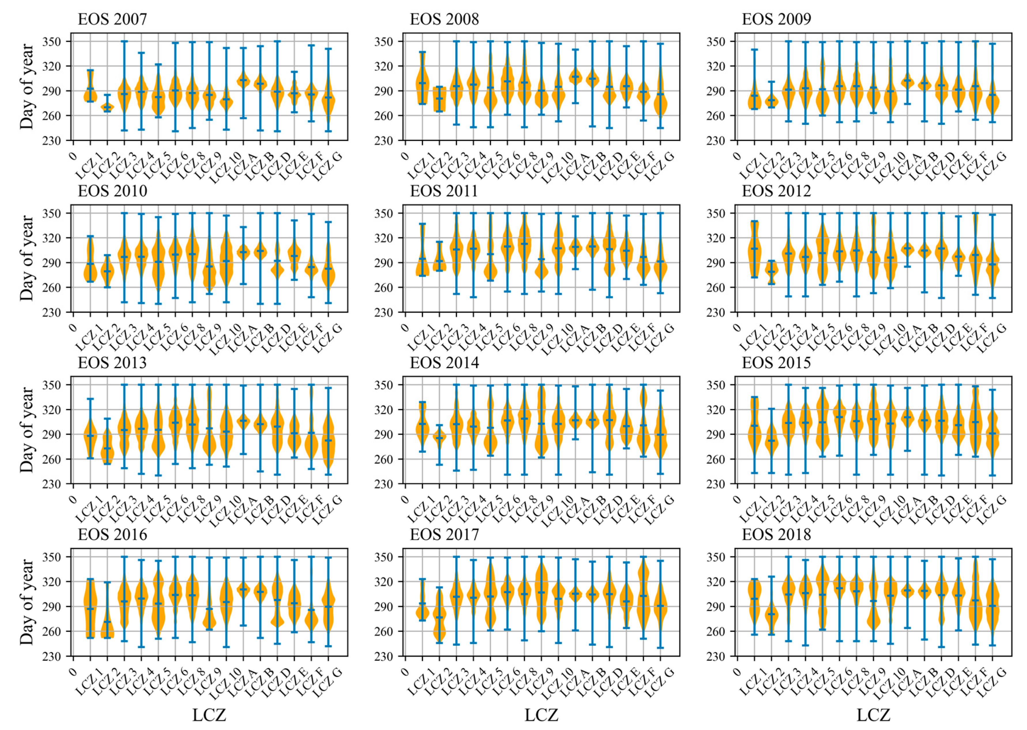
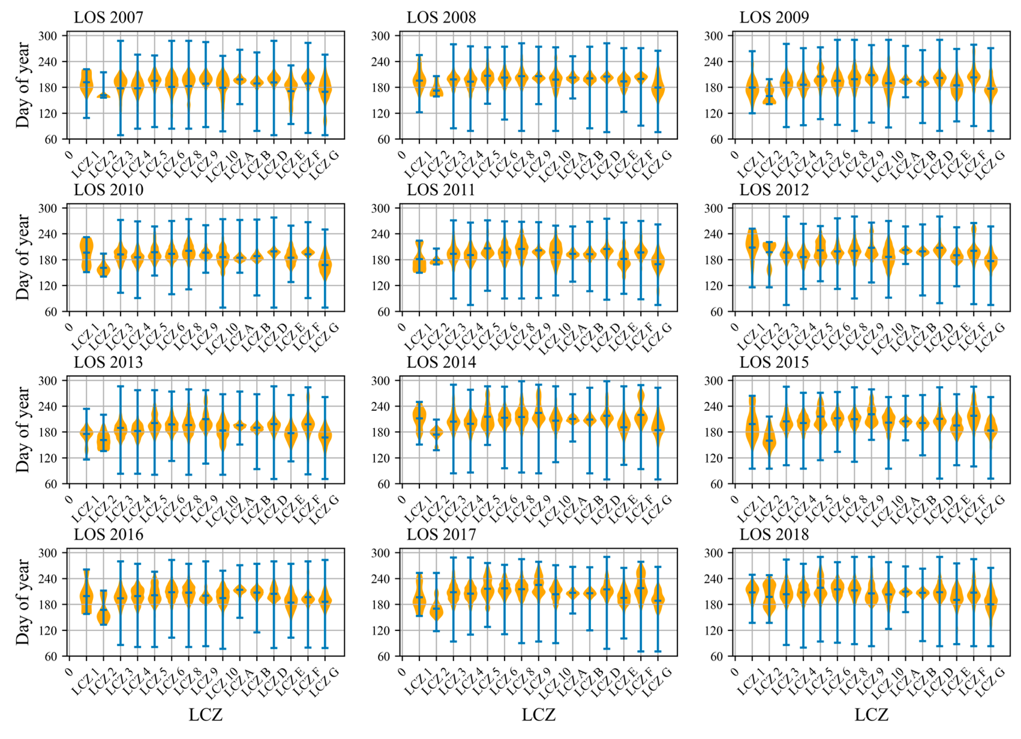
3.2. Distribution of Vegetation Phenology on Various LCZs

Vegetation phenology in different LCZ types was clearly different during the study period, though the variation of phenology on individual LCZ types was not dramatic. Figure 5 and Figure 6 show that SOS and EOS fluctuated significantly along different LCZ classes, with the fluctuation of LOS being smaller (Figure 7), which was most obvious in 2018. Among the natural land cover types, it is evident that the SOS mean distributions on LCZ A and LCZ B were most similar and that the earliest SOS is usually found for the built-up types. The building types were mostly distributed in urban areas, and the air temperature and surface temperature of the building types were generally higher than those of the natural land cover types [57]. The temperature has a crucial effect on vegetation phenology; rising temperature can boost the activity of enzymes and prolong the development of plants [12,18,58,59], consistent with the results of Ren et al. [8].
Typically, the SOS on built-up types preceded natural land cover types. Figure 8a shows the earliest SOS on LCZ 9, which was the 81th day. The longest EOS were mainly clustered on LCZ A and LCZ B in the southern part of the study area (Figure 8b). This may be related to the fact that there were many planted forests in the central and southern part of Jinan. The forest vegetation in Jinan was mainly artificial pure forest, which had simple tree species composition and long-term life cycle. Therefore, the mean value of LOS on LCZ A was the largest, as seen in Figure 8c, and the LOS on LCZ A occurred on day 213 in 2016. In addition to these two types, the average LOS for other built types was high as well, at around 199–208 days.

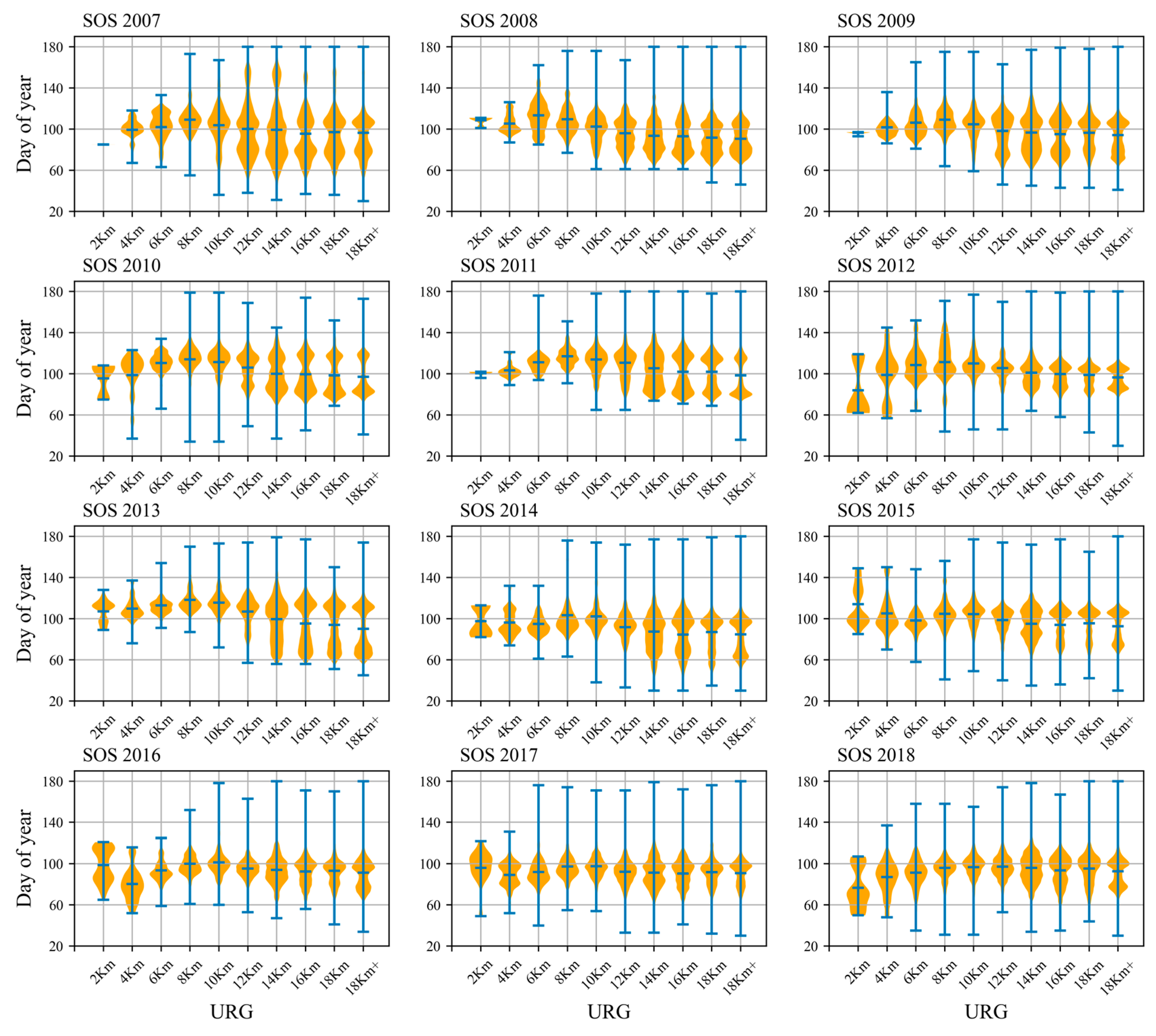
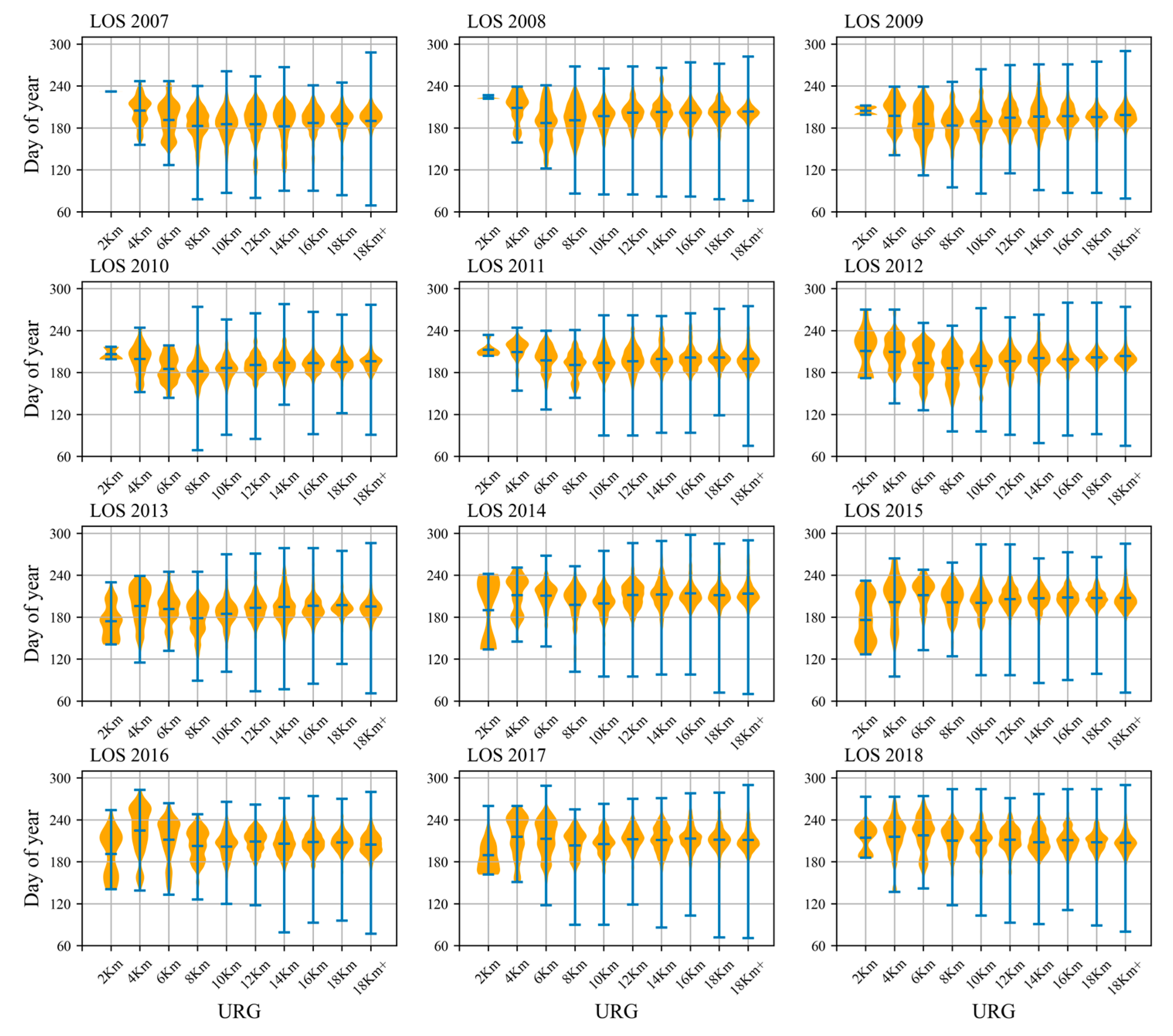
3.3. Distribution of Vegetation Phenology on Various URGs

The distribution of vegetation phenology on different URGs was not widely varied. This might be related to each having a different LCZ type on the gradient (Figure 8d). The SOS mean values fluctuated slightly across the different gradients during the study period, which was all around 100 days. The SOS mean values on 2 km were generally low (Figure 9). The earliest SOS averages were usually found in 2 km or 4 km. For EOS, the mean values on 2 km were generally higher, which was most evident from 2007–2011 (Figure 10). Since 2012, the maximum EOS mean began to appear on 4 km or 6 km. Starting from 4 km, as the gradient increased the EOS mean fluctuated less, and was mostly distributed around 300 days. In general, starting from the urban center, the SOS showed a gradual delay with increasing gradient, while the EOS was gradually advanced (Figure 9 and Figure 10). The distribution of LOS along URGs was similar to that of EOS (Figure 11). The urban center area had a long LOS, and the landscape composition and configuration affected the spatial pattern of vegetation [18]. As in the suburbs in the northern part of Jinan, most EOS and LOS values were distributed around 297 and 200 days in 2016, respectively.

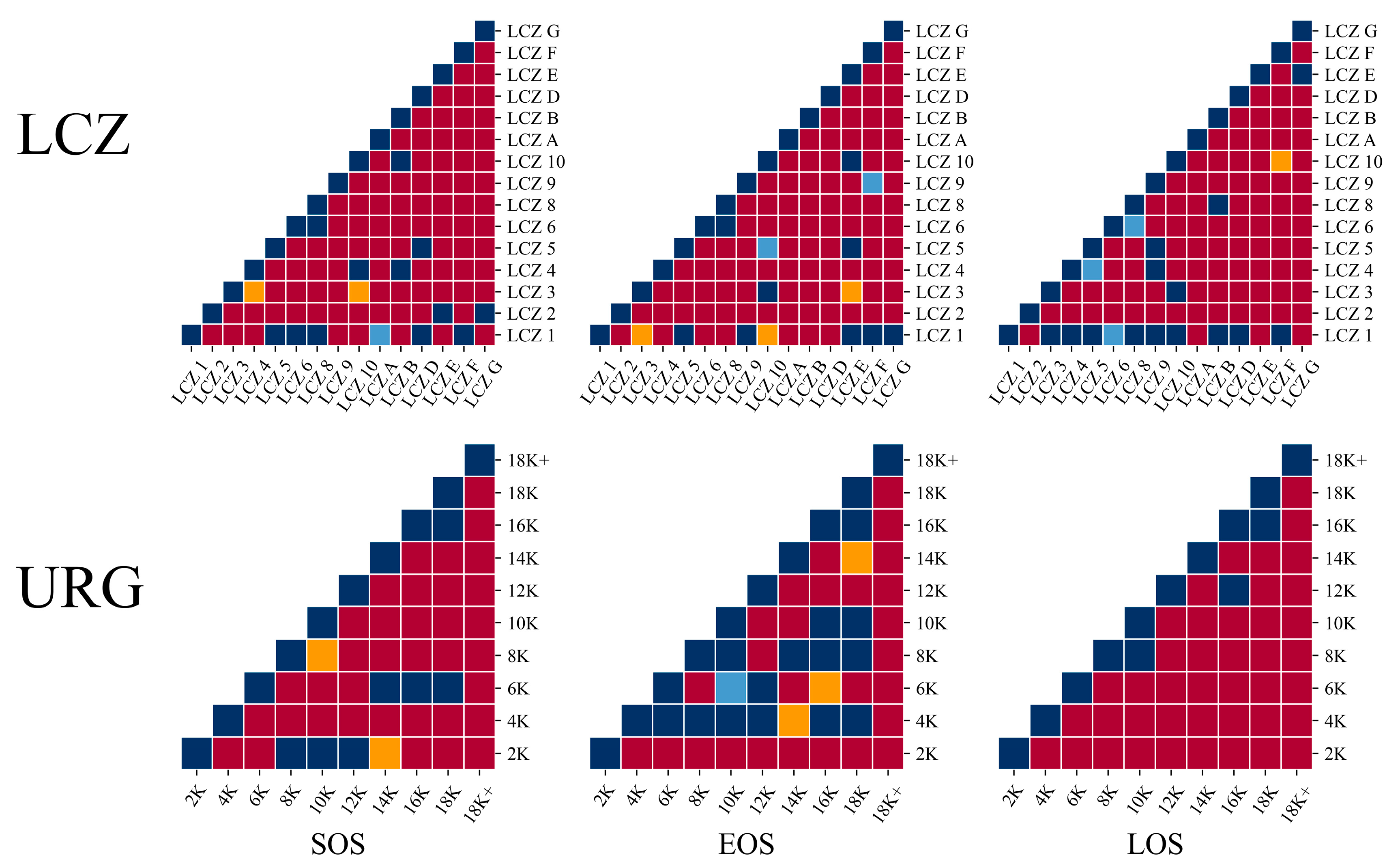
3.4. Comparative Analysis of SOS, EOS, and LOS by LCZ Types and along the URGs

Because the LCZ classification map of 2016 was used in this study, when using the HSD test it was more accurate to detect the difference between the LCZs and URGs of vegetation phenology in 2016. The results showed that the variability of vegetation phenology was larger for different LCZ types. The LCZ logarithms with significant differences in SOS, EOS, and LOS were 93, 96, and 91, respectively, while the logarithms of URG with distinct differences were 38, 31, and 42, respectively. The squares in dark blue represent no remarkable difference between the vegetation phenology of these LCZ pairs and URG pairs (Figure 12). The differences of the other squares in the figure are shown as red, orange, and light blue in descending order. The proportion of LCZ pairs with variability in EOS was 80.0%, 23.6% more than that in URG pairs (Table 1). This variability was not as obvious in LOS, where it was the largest in EOS, followed by SOS.

4. Discussion

Urban vegetation phenology often differed between urban and rural areas, and the URG method was better able to consider the differences between urban and rural areas, revealing the impact of urbanization on vegetation phenology [11,60]. However, the URG only took the urban center as the starting point, and analyzed the changes in vegetation phenology from the horizontal distance [55] without considering the influence of vertical factors. LCZ considers the three-dimensional characteristics of buildings a swell as the classification and functional zoning of urban buildings, and uses building height, building density, and other information to describe the urban canopy. Compared with traditional land classification methods, the LCZ classification scheme standardizes urban form and functional zoning, which play a crucial role in urban phenological research.
Due to the influence of meteorological factors and cloud cover, the MODIS data might contain missing values and outliers. For the outliers in phenological data, we adopted thresholding to eliminate the values less than 30 days or more than 180 days in SOS and less than 240 days or more than 350 days in EOS. In this process, the threshold value was influenced by the climate and vegetation characteristics of the study area, and some analysis results needed to be avoided due to missing data. Therefore, areas with missing values appear in Figure 2 and Figure 3, mainly those belonging to the LCZ D category or those outside 18 K, which had little impact on the analysis of interannual trends in vegetation phenology in the study area. During the study period, SOS, EOS, and LOS in Jinan showed an earlier, later, and longer trend, respectively (Figure 4). This is consistent with previous findings on the interannual variation of vegetation phenology [8,9,18]. Global climate change is one of the main reasons for the advance of vegetation SOS [61] and the delay of EOS [58]. Climate warming leads to an increase in temperature, which in turn prolongs the vegetation growth cycle [58,59]. The increase in atmospheric CO2 concentration and adequate soil moisture results in SOS trends and delay in the advance of EOS. Land use change and human activities can alter vegetation ecosystems and affect vegetation phenology [12].
The MCD12Q2 dataset we used had an annual temporal resolution and a spatial resolution of 500 m. This low spatial and temporal resolution might not capture the subtle vegetation changes and intra-urban vegetation differences required for urban vegetation climate studies. Therefore, when using the dataset, it is essential to choose appropriate remote sensing indicators or integrate other remote sensing data for data fusion in order to obtain more accurate vegetation phenology information. Opportunities are emerging with new spatial data and technologies to monitor spatiotemporal patterns of phenology and environmental factors within and across cities. Phenology indicators based on sun-induced chlorophyll fluorescence are better proxies of photosynthetic activities compared to traditional greenness phenology data [62,63], while urban phenology indicators derived from high spatial resolution satellite observations such as Landsat can better capture heterogeneous information in complex urban environments [64]. The recently developed Black Marble night-time lights product [65] and gridded air temperature dataset [66] provide novel data to study the impact of artificial light and temperature on phenology. These novel technologies and datasets show promise to help disentangle the complex mechanisms of urban phenology changes.

5. Conclusions

In this study, by connecting vegetation phenology indexes (SOS, EOS, and LOS) with URG information and the LCZ classification system for urban land, the temporal and spatial distribution of urban vegetation phenology in Jinan City was explored. It was found that the SOS and EOS in study area were advanced and delayed by an average of 0.46d·(10a)−1 and 10.3d·(10a)−1, respectively, while the LOS lengthened by an average of 14.4d·(10a)−1. There were obvious differences in SOS and EOS among different LCZ types. The vegetation phenology of LCZ pairs showed more remarkable differences than that of URG pairs. In SOS, EOS, and LOS, the proportion of LCZ pairs and URG pairs with differences was (77.5%, 80.0%, 75.8%) and (69.1%, 56.4%, 76.4%), respectively.
The URG only considers the distribution changes of vegetation phenology from a horizontal perspective, ignoring the three-dimensional structure of the city. In contrast, the LCZ classification system considers that cities have three-dimensional characteristics in the form of buildings and that the surface materials of different buildings in cities are different. This provides a new research idea for the study of urban vegetation phenology and its response to urbanization. The present study illustrates the temporal and spatial distribution characteristics of urban vegetation phenology and the influence of urbanization on vegetation phenology, which can play a crucial role in comparing and evaluating the impact of different decisions on the urban environment, thereby providing a decision-making basis for scientific governance and contributing to the sustainable and healthy development of cities.

Author Contributions

S.L. Data curation, investigation, software, code, writing—original draft; Q.L. code, software, writing—review, formal analysis, writing—review; J.Z. conceptualization, funding acquisition, supervision; writing—review; S.Z. (Shichao Zhang) code, software, writing—review, formal analysis; X.W. software, visualization, writing—review; S.Y. visualization, writing—review; S.Z. (Sha Zha) writing—review. All authors have read and agreed to the published version of the manuscript.

Funding

This work was jointly supported by the Central Guiding Local Science and Technology Development Fund of Shandong—Yellow River Basin Collaborative Science and Technology Innovation Special Project “Study on the Prediction Technology and Countermeasures of Compound High Temperature and Drought in Ningxia” (No. YDZX2023019), Shandong Natural Science Foundation of China (No. 2018GNC110025, No. ZR2020QE281), and “Taishan Scholar” Project of Shandong Province (No. TSXZ201712).

Institutional Review Board Statement

Not applicable.

Informed Consent Statement

Not applicable.

Data Availability Statement

Not applicable.

Acknowledgments

The authors would like to acknowledge the valuable comments on the manuscript provided by the anonymous reviewers and editor.

Conflicts of Interest

The authors declare no conflict of interest.

References

  1. Sarvia, F.; De Petris, S.; Borgogno Mondino, E. Exploring Climate Change Effects on Vegetation Phenology by MOD13Q1 Data: The Piemonte Region Case Study in the Period 2001–2019. Agronomy 2021, 11, 555. [Google Scholar] [CrossRef]
  2. Zhou, Y. Understanding urban plant phenology for sustainable cities and planet. Nat. Clim. Chang. 2022, 12, 302–304. [Google Scholar] [CrossRef]
  3. Linderholm, H. Growing Season Changes in the Last Century. Agric. For. Meteorol. 2006, 137, 1–14. [Google Scholar] [CrossRef]
  4. Chen, X.; Hu, B.; Yu, R. Spatial and temporal variation of phenological growing season and climate change impacts in temperate eastern China. Glob. Chang. Biol. 2005, 11, 1118–1130. [Google Scholar] [CrossRef]
  5. Morisette, J.; Richardson, A.; Knapp, A.; Graham, E.; Abnatzoglou, J.; Wilson, B.; Breshears, D.; Henebry, G.; Hanes, J.; Liang, L. Tracking the rhythm of the seasons in the face of global change: Phenological research in the 21st century. Front. Ecol. Environ. 2009, 7, 253–260. [Google Scholar] [CrossRef]
  6. Tang, H.; Li, Z.; Chen, B.; Zhang, B.; Xin, X. Variability and Climate Change Trend in Vegetation Phenology of Recent Decades in the Greater Khingan Mountain Area, Northeastern China. Remote Sens. 2015, 7, 11914–11932. [Google Scholar] [CrossRef]
  7. Wang, X.; Gao, Q.; Wang, C.; Yu, M. Spatiotemporal patterns of vegetation phenology change and relationships with climate in the two transects of East China. Glob. Ecol. Conserv. 2017, 10, 206–219. [Google Scholar] [CrossRef]
  8. Ren, Q.; He, C.; Huang, Q.; Zhou, Y. Urbanization Impacts on Vegetation Phenology in China. Remote Sens. 2018, 10, 1905. [Google Scholar] [CrossRef]
  9. Xuecao, L.; Zhou, Y.; Asrar, G.; Mao, J.; Li, X.; Li, W. Response of vegetation phenology to urbanization in the conterminous United States. Glob. Chang. Biol. 2017, 23, 2818–2830. [Google Scholar] [CrossRef]
  10. Su, Y.; Liu, L.; Liao, J.; Wu, J.; Ciais, P.; Liao, J.; He, X.; Liu, X.; Chen, X.; Yuan, W.; et al. Phenology acts as a primary control of urban vegetation cooling and warming: A synthetic analysis of global site observations. Agric. For. Meteorol. 2020, 280, 107765. [Google Scholar] [CrossRef]
  11. Luo, X.; Zhang, Y.; Sun, D. Response Patterns of Vegetation Phenology along Urban-Rural Gradients in Urban Areas of Different Sizes. Complexity 2020, 2020, 1–11. [Google Scholar] [CrossRef]
  12. Ji, Y.; Jin, J.; Zhan, W.; Guo, F.; Yan, T. Quantification of Urban Heat Island-Induced Contribution to Advance in Spring Phenology: A Case Study in Hangzhou, China. Remote Sens. 2021, 13, 3684. [Google Scholar] [CrossRef]
  13. Li, D.; Wu, S.; Liang, Z.; Li, S. The impacts of urbanization and climate change on urban vegetation dynamics in China. Urban For. Urban Green. 2020, 54, 126764. [Google Scholar] [CrossRef]
  14. Wang, R.; Ren, C.; Xu, Y.; Lau, K.; Shi, Y. Mapping the local climate zones of urban areas by GIS-based and WUDAPT methods: A case study of Hong Kong. Urban Clim. 2018, 24, 567–576. [Google Scholar] [CrossRef]
  15. Stewart, I.D.; Oke, T. Local Climate Zones for Urban Temperature Studies. Bull. Am. Meteorol. Soc. 2012, 93, 1879–1900. [Google Scholar] [CrossRef]
  16. Zhou, D.; Zhao, S.; Zhang, L.; Liu, S. Remotely sensed assessment of urbanization effects on vegetation phenology in China’s 32 major cities. Remote Sens. Environ. 2016, 176, 272–281. [Google Scholar] [CrossRef]
  17. Zhang, Y.; Yin, P.; Li, X.; Niu, Q.; Wang, Y.; Cao, W.; Huang, J.; Chen, H.; Yao, X.; Yu, L. The divergent response of vegetation phenology to urbanization: A case study of Beijing city, China. Sci. Total Environ. 2022, 803, 150079. [Google Scholar] [CrossRef]
  18. Qiu, T.; Song, C.; Li, J. Impacts of Urbanization on Vegetation Phenology over the Past Three Decades in Shanghai, China. Remote Sens. 2017, 9, 970. [Google Scholar] [CrossRef]
  19. Parece, T.; Campbell, J. Intra-Urban Microclimate Effects on Phenology. Urban Sci. 2018, 2, 26. [Google Scholar] [CrossRef]
  20. Wang, J.; Sun, H.; Xiong, J.; He, D.; Cheng, W.; Ye, C.; Yong, Z.; Huang, X. Dynamics and Drivers of Vegetation Phenology in Three-River Headwaters Region Based on the Google Earth Engine. Remote Sens. 2021, 13, 2528. [Google Scholar] [CrossRef]
  21. Wu, Q. geemap: A Python package for interactive mapping with Google Earth Engine. J. Open Source Softw. 2020, 5, 2305. [Google Scholar] [CrossRef]
  22. Yang, L.; Zhao, S. A stronger advance of urban spring vegetation phenology narrows vegetation productivity difference between urban settings and natural environments. Sci. Total Environ. 2023, 868, 161649. [Google Scholar] [CrossRef]
  23. Jiao, F.; Liu, H.; Xu, X.; Gong, H.; Lin, Z. Trend Evolution of Vegetation Phenology in China during the Period of 1981–2016. Remote Sensing 2020, 12, 572. [Google Scholar] [CrossRef]
  24. Zhang, R.; Qi, J.; Leng, S.; Wang, Q. Long-Term Vegetation Phenology Changes and Responses to Preseason Temperature and Precipitation in Northern China. Remote Sens. 2022, 14, 1396. [Google Scholar] [CrossRef]
  25. Li, C.; Zou, Y.; He, J.; Zhang, W.; Gao, L.; Zhuang, D. Response of Vegetation Phenology to the Interaction of Temperature and Precipitation Changes in Qilian Mountains. Remote Sens. 2022, 14, 1248. [Google Scholar] [CrossRef]
  26. Shi, Y.; Jin, N.; Ma, X.; Wu, B.; He, Q.; Yue, C.; Yu, Q. Attribution of climate and human activities to vegetation change in China using machine learning techniques. Agric. For. Meteorol. 2020, 294, 108146. [Google Scholar] [CrossRef]
  27. Quan, S.J.; Dutt, F.; Woodworth, E.; Yamagata, Y.; Yang, P.P.-J. Local climate zone mapping for energy resilience: A fine-grained and 3D approach. Energy Procedia 2017, 105, 3777–3783. [Google Scholar] [CrossRef]
  28. Geletič, J.; Lehnert, M.; Savić, S.; Milošević, D. Inter-/intra-zonal seasonal variability of the surface urban heat island based on local climate zones in three central European cities. Build. Environ. 2019, 156, 21–32. [Google Scholar] [CrossRef]
  29. Liu, S.; Qi, Z.; Li, X.; Yeh, A.G.-O. Integration of convolutional neural networks and object-based post-classification refinement for land use and land cover mapping with optical and SAR data. Remote Sens. 2019, 11, 690. [Google Scholar] [CrossRef]
  30. Qiu, C.; Tong, X.; Schmitt, M.; Bechtel, B.; Zhu, X.X. Multilevel feature fusion-based CNN for local climate zone classification from sentinel-2 images: Benchmark results on the So2Sat LCZ42 dataset. IEEE J. Sel. Top. Appl. Earth Obs. Remote Sens. 2020, 13, 2793–2806. [Google Scholar] [CrossRef]
  31. Danylo, O.; See, L.; Bechtel, B.; Schepaschenko, D.; Fritz, S. Contributing to WUDAPT: A Local Climate Zone Classification of Two Cities in Ukraine. IEEE J. Sel. Top. Appl. Earth Obs. Remote Sens. 2016, 9, 1841–1853. [Google Scholar] [CrossRef]
  32. Bechtel, B.; See, L.; Mills, G.; Foley, M. Classification of Local Climate Zones Using SAR and Multispectral Data in an Arid Environment. IEEE J. Sel. Top. Appl. Earth Obs. Remote Sens. 2016, 9, 3097–3105. [Google Scholar] [CrossRef]
  33. Demuzere, M.; Bechtel, B.; Middel, A.; Mills, G. Mapping Europe into local climate zones. PLoS ONE 2019, 14, e0214474. [Google Scholar] [CrossRef]
  34. Cai, M.; Ren, C.; Xu, Y.; Lau, K.K.-L.; Wang, R. Investigating the relationship between local climate zone and land surface temperature using an improved WUDAPT methodology—A case study of Yangtze River Delta, China. Urban Clim. 2018, 24, 485–502. [Google Scholar] [CrossRef]
  35. Ren, C.; Cai, M.; Li, X.; Zhang, L.; Wang, R.; Xu, Y.; Ng, E. Assessment of local climate zone classification maps of cities in China and feasible refinements. Sci. Rep. 2019, 9, 18848. [Google Scholar] [CrossRef]
  36. Jia, W.; Zhao, S.; Liu, S. Vegetation growth enhancement in urban environments of the Conterminous United States. Glob. Chang. Biol. 2018, 24, 4084–4094. [Google Scholar] [CrossRef]
  37. Jia, W.; Zhao, S.; Zhang, X.; Liu, S.; Henebry, G.; Liu, L. Urbanization imprint on land surface phenology: The urban–rural gradient analysis for Chinese cities. Glob. Chang. Biol. 2021, 27, 2895–2904. [Google Scholar] [CrossRef]
  38. Feng, l.; Song, G.; Zhu, L.; Xiuqin, F.; Yanan, Z. Urban vegetation phenology analysis and the response to the temperature change. In Proceedings of the 2017 IEEE International Geoscience and Remote Sensing Symposium (IGARSS), Fort Worth, TX, USA, 23–28 July 2017; pp. 5743–5746. [Google Scholar]
  39. Cancan, Y.; Deng, K.; Peng, D.; Jiang, L.; Mingwei, Z.; Liu, J.; Qiu, X. Spatiotemporal Characteristics and Heterogeneity of Vegetation Phenology in the Yangtze River Delta. Remote Sens. 2022, 14, 2984. [Google Scholar] [CrossRef]
  40. Zhang, X.; Friedl, M.; Schaaf, C.; Strahler, A.; Schneider, A. The footprint of urban climates on vegetation phenology. Geophys. Res. Lett 2004, 31. [Google Scholar] [CrossRef]
  41. Ullah, M.; Li, J.; Wadood, B. Analysis of Urban Expansion and its Impacts on Land Surface Temperature and Vegetation Using RS and GIS, A Case Study in Xi’an City, China. Earth Syst. Environ. 2020, 4, 583–597. [Google Scholar] [CrossRef]
  42. Li, P.; Sun, M.; Liu, Y.; Ren, P.; Peng, C.; Zhou, X.; Tang, J. Response of Vegetation Photosynthetic Phenology to Urbanization in Dongting Lake Basin, China. Remote Sens. 2021, 13, 3722. [Google Scholar] [CrossRef]
  43. Tao, J.; Kong, X.; Wang, Y.; Chen, R. A study of vegetation phenology in the analysis of urbanization process based on time-series MODIS data. In Proceedings of the 2016 IEEE International Geoscience and Remote Sensing Symposium (IGARSS), Beijing, China, 10–15 July 2016; pp. 2826–2829. [Google Scholar]
  44. Melaas, E.; Wang, J.; Miller, D.; Friedl, M. Interactions between urban vegetation and surface urban heat islands: A case study in the Boston metropolitan region. Environ. Res. Lett. 2016, 11, 054020. [Google Scholar] [CrossRef]
  45. Burnett, M.; Chen, D. Urban Heat Island Footprint Effects on Bio-Productive Rural Land Covers Surrounding a Low Density Urban Center. Int. Arch. Photogramm. Remote Sens. Spat. Inf. Sci. 2021, 43, 539–550. [Google Scholar] [CrossRef]
  46. Li, N.; Yang, J.; Qiao, Z.; Wang, Y.; Miao, S.; Nichol, J.; Wang, Q. Urban Thermal Characteristics of Local Climate Zones and Their Mitigation Measures across Cities in Different Climate Zones of China. Remote Sens. 2021, 13, 1468. [Google Scholar] [CrossRef]
  47. Del Pozo, S.; Landes, T.; Nerry, F.; Kastendeuch, P.; Najjar, G.; Philipps, N.; Lagüela, S. Evaluation of the seasonal nighttime LST-air temperature discrepancies and their relation to local climate zones (LCZ) in strasbourg. Int. Arch. Photogramm. Remote Sens. Spat. Inf. Sci. 2021, XLIII-B3-2021, 391–398. [Google Scholar] [CrossRef]
  48. Hu, J.; Yang, Y.; Pan, X.; Zhu, Q.; Zhan, W.; Wang, Y.; Ma, W.; Su, W. Analysis of the Spatial and Temporal Variations of Land Surface Temperature Based on Local Climate Zones: A Case Study in Nanjing, China. IEEE J. Sel. Top. Appl. Earth Obs. Remote Sens. 2019, 12, 4213–4223. [Google Scholar] [CrossRef]
  49. Zhang, Y.; Bambrick, H.; Mengersen, K.; Tong, S.; Feng, L.; Zhang, L.; Liu, G.; Xu, A.; Hu, W. Using big data to predict pertussis infections in Jinan city, China: A time series analysis. Int. J. Biometeorol. 2020, 64, 95–104. [Google Scholar] [CrossRef]
  50. Zhang, J.; Su, Y.-R.; Wu, J.; Liang, H. GIS based land suitability assessment for tobacco production using AHP and fuzzy set in Shandong province of China. Comput. Electron. Agric. 2015, 114, 202–211. [Google Scholar] [CrossRef]
  51. Lin, S.; Ruan, S.; Geng, X.; Song, K.; Cui, L.-L.; Liu, X.; Zhang, Y.; Cao, M.; Zhang, Y. Non-linear relationships and interactions of meteorological factors on mumps in Jinan, China. Int. J. Biometeorol. 2021, 65, 555–563. [Google Scholar] [CrossRef] [PubMed]
  52. Li, M.; Hu, B.; Zhang, B. Evolution of urban built-up areas and its impact on urban vegetation of Jinan City, Eastern China. In Proceedings of the 2022 29th International Conference on Geoinformatics, Beijing, China, 15–18 August 2022; pp. 1–8. [Google Scholar]
  53. Ganguly, S.; Friedl, M.; Tan, B.; Zhang, X.; Verma, M. Land surface phenology from MODIS: Characterization of the Collection 5 Global Land Cover Dynamics Product. Remote Sens. Environ. 2010, 114, 1805–1816. [Google Scholar] [CrossRef]
  54. Zhang, X.; Friedl, M.; Schaaf, C. Global vegetation phenology from Moderate Resolution Imaging Spectroradiometer (MODIS): Evaluation of global patterns and comparison with in situ measurements. J. Geophys. Res. 2006, 111. [Google Scholar] [CrossRef]
  55. Zhao, C.; Weng, Q.; Wang, Y.; Hu, Z.; Wu, C. Use of local climate zones to assess the spatiotemporal variations of urban vegetation phenology in Austin, Texas, USA. GIScience Remote Sens. 2022, 59, 393–409. [Google Scholar] [CrossRef]
  56. Nanda, A.; Mohapatra, B.B.; Mahapatra, A.P.K.; Mahapatra, A.P.K.; Mahapatra, A. Multiple comparison test by Tukey’s honestly significant difference (HSD): Do the confident level control type I error. Int. J. Stat. Appl. Math. 2021, 6, 59–65. [Google Scholar] [CrossRef]
  57. Jiang, S.; Zhan, W.; Yang, J.; Liu, Z.; Huang, F.; Lai, M.; Li, J.; Hong, F.; Huang, Y.; Chen, J.; et al. Urban heat island studies based on local climate zones: A systematic overview. Acta Geogr. Sin. 2020, 75, 1860–1878. [Google Scholar] [CrossRef]
  58. Richardson, A.D.; Keenan, T.F.; Migliavacca, M.; Ryu, Y.; Sonnentag, O.; Toomey, M. Climate change, phenology, and phenological control of vegetation feedbacks to the climate system. Agric. For. Meteorol. 2013, 169, 156–173. [Google Scholar] [CrossRef]
  59. Keenan, T.; Gray, J.; Friedl, M.; Toomey, M.; Bohrer, G.; Hollinger, D.; Munger, J.; O’Keefe, J.; Schmid, H.; Wing, I.; et al. Net carbon uptake has increased through warming-induced changes in temperate forest phenology. Nat. Clim. Chang. 2014, 4, 598–604. [Google Scholar] [CrossRef]
  60. Yang, J.; Luo, X.; Jin, C.; Xiao, X.; Xia, J.C. Spatiotemporal patterns of vegetation phenology along the urban–rural gradient in Coastal Dalian, China. Urban For. Urban Green. 2020, 54, 126784. [Google Scholar] [CrossRef]
  61. Körner, C.; Basler, D. Phenology under global warming. Science 2010, 327, 1461–1462. [Google Scholar] [CrossRef]
  62. Zhao, D.; Hou, Y.; Zhang, Z.; Wu, Y.; Zhang, X.; Wu, L.; Zhu, X.; Zhang, Y. Temporal resolution of vegetation indices and solar-induced chlorophyll fluorescence data affects the accuracy of vegetation phenology estimation: A study using in-situ measurements. Ecol. Indic. 2022, 136, 108673. [Google Scholar] [CrossRef]
  63. Wang, S.; Ju, W.; Peñuelas, J.; Cescatti, A.; Zhou, Y.; Fu, Y.; Huete, A.; Liu, M.; Zhang, Y. Urban-rural gradients reveal joint control of elevated CO2 and temperature on extended photosynthetic seasons. Nat. Ecol. Evol. 2019, 3, 1076–1085. [Google Scholar] [CrossRef]
  64. Li, X.; Zhou, Y.; Meng, L.; Asrar, G.R.; Lu, C.; Wu, Q. A dataset of 30 m annual vegetation phenology indicators (1985–2015) in urban areas of the conterminous United States. Earth Syst. Sci. Data 2019, 11, 881–894. [Google Scholar] [CrossRef]
  65. Román, M.O.; Wang, Z.; Sun, Q.; Kalb, V.; Miller, S.D.; Molthan, A.; Schultz, L.; Bell, J.; Stokes, E.C.; Pandey, B. NASA’s Black Marble nighttime lights product suite. Remote Sens. Environ. 2018, 210, 113–143. [Google Scholar] [CrossRef]
  66. Li, X.; Zhou, Y.; Asrar, G.R.; Zhu, Z. Developing a 1 km resolution daily air temperature dataset for urban and surrounding areas in the conterminous United States. Remote Sens. Environ. 2018, 215, 74–84. [Google Scholar] [CrossRef]
Figure 1. Location of the study area (a) and LCZ types (the circles in (b) represent the distance from the urban center, starting from the smallest circle in the order of 2 Kilometers, 4 Kilometers, 6 Kilometers, 8 Kilometers, 10 Kilometers, 12 Kilometers, 14 Kilometers, 16 Kilometers, 18 Kilometers, 18 Kilometers + (the area in the study area except the largest circle)).
Remotesensing 15 03957 g001
Figure 2. Spatial distributions of (a) SOS, (b) EOS, and (c) LOS in the study area from 2007–2018; the default values are caused by the elimination of effects such as clouds or by outliers of phenological parameters that do not exist within the defined threshold conditions.
Remotesensing 15 03957 g002
Figure 3. Spatial distribution of interannual trends in (a) SOS, (b) EOS, and (c) LOS in the study area from 2007–2018; the default values are caused by the elimination of effects such as clouds or by outliers of phenological parameters that do not exist within the defined threshold conditions.
Remotesensing 15 03957 g003
Figure 4. Interannual variation of (a) SOS, (b) EOS, and (c) LOS in the study area from 2007–2018. (The blue dots correspond to the mean value of a certain year’s phenological indicator, and the blue lines represent the linear regression line of these dots).
Remotesensing 15 03957 g004
Figure 5. Violin plot of the SOS distribution based on different LCZs from 2007 to 2018. The shape of the yellow area reflects the density distribution of the data; the top line shows the maximum, the center line shows the average, and the bottom line shows the minimum.
Remotesensing 15 03957 g005
Figure 6. Violin plot of the EOS distribution based on different LCZs from 2007 to 2018. The shape of the yellow area reflects the density distribution of the data; the top line shows the maximum, the center line shows the average, and the bottom line shows the minimum.
Remotesensing 15 03957 g006
Figure 7. Violin plot of the LOS distribution based on different LCZs from 2007 to 2018. The shape of the yellow area reflects the density distribution of the data; the top line shows the maximum, the center line shows the average, and the bottom line shows the minimum.
Remotesensing 15 03957 g007
Figure 8. Phenological mean ((a) SOS, (b) EOS, (c) LOS) distribution on URGs and LCZs in 2016 and (d) LCZs along URGs in 2016.
Remotesensing 15 03957 g008
Figure 9. Violin plot of the SOS distribution based on different URGs from 2007 to 2018. The shape of the yellow area reflects the density distribution of the data; the top line shows the maximum, the center line shows the average, and the bottom line shows the minimum.
Remotesensing 15 03957 g009
Figure 10. Violin plot of the EOS distribution based on different URGs from 2007 to 2018. The shape of the yellow area reflects the density distribution of the data; the top line shows the maximum, the center line shows the average, and the bottom line shows the minimum.
Remotesensing 15 03957 g010
Figure 11. Violin plot of the LOS distribution based on different URGs from 2007 to 2018. The shape of the yellow area reflects the density distribution of the data; the top line shows the maximum, the center line shows the average, and the bottom line shows the minimum.
Remotesensing 15 03957 g011
Figure 12. HSD test results of SOS, EOS, and LOS based on LCZ and URG in 2016. Dark blue represents no significant difference, while red, orange, and light blue represent significant differences with significance levels of 0.001, 0.01, and 0.05, respectively).
Remotesensing 15 03957 g012
Table 1. The proportion of LCZ pairs and URG pairs with significant differences in SOS, EOS, and LOS in 2016.
SOSEOSLOS
LCZ77.5%80.0%75.8%
URG69.1%56.4%76.4%
Difference8.4%23.6%−0.6%
Disclaimer/Publisher’s Note: The statements, opinions and data contained in all publications are solely those of the individual author(s) and contributor(s) and not of MDPI and/or the editor(s). MDPI and/or the editor(s) disclaim responsibility for any injury to people or property resulting from any ideas, methods, instructions or products referred to in the content.

