A Parametric Study of MPSO-ANN Techniques in Gas-Bearing Distribution Prediction Using Multicomponent Seismic Data

Abstract

Predicting the oil–gas-bearing distribution of unconventional reservoirs is challenging because of the complex seismic response relationship of these reservoirs. Artificial neural network (ANN) technology has been popular in seismic reservoir prediction because of its self-learning and nonlinear expression abilities. However, problems in the training process of ANNs, such as slow convergence speed and local minima, affect the prediction accuracy. Therefore, this study proposes a hybrid prediction method that combines mutation particle swarm optimization (MPSO) and ANN (MPSO-ANN). It uses the powerful search ability of MPSO to address local optimization problems during training and improve the performance of ANN models in gas-bearing distribution prediction. Furthermore, because the predictions of ANN models require good data sources, multicomponent seismic data that can provide rich gas reservoir information are used as input for MPSO-ANN learning. First, the hyperparameters of the ANN model were analyzed, and ANNs with different structures were constructed. The initial ANN model before optimization exhibited good predictive performance. Then, the parameter settings of MPSO were analyzed, and the MPSO-ANN model was obtained by using MPSO to optimize the weights and biases of the developed ANN model. Finally, the gas-bearing distribution was predicted using multicomponent seismic data. The results indicate that the developed MPSO-ANN model (MSE = 0.0058, RMSE = 0.0762, R² = 0.9761) has better predictive performance than the PSO-ANN (MSE = 0.0062, RMSE = 0.0786, R² = 0.9713) and unoptimized ANN models (MSE = 0.0069, RMSE = 0.0833, R² = 0.9625) on the test dataset. Additionally, the gas-bearing distribution prediction results were consistent overall with the actual drilling results, further verifying the feasibility of this method. The research results may contribute to the application of PSO and ANN in reservoir prediction and other fields.

1. Introduction

Unconventional or dispersed gas is stored in unconventional reservoirs with complex geology. Compared with conventional gas reservoirs, they have more diverse types and forms of occurrence, with wider distribution ranges and much larger potential resources. Owing to the particular accumulation and occurrence conditions of unconventional gas reservoirs, their seismic response characteristics are complex and unclear, making reservoir characterization and prediction based on seismic information difficult. Therefore, developing new methods to predict unconventional gas reservoirs is extremely important [1,2,3].

A large amount of data has been generated to explore unconventional reservoirs and must be effectively utilized to establish data-driven reservoir prediction methods [4,5]. Data-driven models are expected to derive several highly nonlinear and multifactorial interaction relationships between inputs and outputs from the obtained data [6,7]. Compared with conventional process-driven models, they focus more on data analysis and applications, and it is not necessary to oversimplify or ignore most factors, as required by physical modeling [8]. Machine learning (ML) can process nonlinear data and automatically learn highly nonlinear relationships between the target and input parameters from the input data. Therefore, data-driven models rely on ML methods. Using the self-learning characteristics of various ML methods, patterns hidden in the data can be mined to predict unknown situations using the learned patterns. Various ML methods have been applied to reservoir prediction, including artificial neural networks (ANNs) [9,10], support vector machines [11,12], decision trees [13,14], cluster analysis [15,16], and deep learning [17,18].

Among them, ANNs are most typically used and are widely used for reservoir prediction [19,20,21] because they can accurately model fuzzy and nonlinear problems [22,23,24,25]. Wang et al. [26] used an ANN to reveal the internal relationship between the reservoir physical parameters and rock physical logging to predict reservoir porosity accurately. Zheng et al. [27] extracted the complex relationship between the logging curve and total organic carbon (TOC) value using an ANN and established an accurate TOC prediction model. Despite the accurate predictions of ANNs, the large randomness in their initial value selection causes problems in practical applications, such as a slow convergence speed and long training time, resulting in low accuracy. Therefore, the neural network requires optimization. Various optimization algorithms are used for this purpose, such as the backpropagation algorithm [28], particle swarm optimization (PSO) algorithm [29,30,31], genetic algorithm (GA) [32,33], and imperialist competitive algorithm [34,35]. Ouadfeul and Aliouane [36] used the Levenberg–Marquardt algorithm (LMA) to optimize an ANN, which was then used to predict the TOC content of the Barnett Shale gas field. Chanda and Singh [37] used a GA to optimize an ANN to predict the gas production potential of methane hydrate reservoirs. Mahmoodpour et al. [38] used a PSO-ANN to predict the cementation coefficient of a low-permeability carbonate reservoir. Among these optimization algorithms, PSO is easy to implement and has a fast convergence speed while ensuring high prediction accuracy.

As mentioned above, various ANN models (with or without optimization) are used for reservoir prediction, but they are unsuitable for some purposes, in particular multicomponent seismic reservoir prediction. Additionally, PSO tends to fall into local extreme values, affecting its optimization ability. Therefore, this study proposes a hybrid prediction method that combines mutated PSO (MPSO) and ANN (MPSO-ANN) for gas reservoir prediction. In addition, the structure of ANN also significantly affects model performance. Therefore, this study first analyzed the hyperparameters of the ANN to determine the network structure of the unoptimized initial ANN. Then, its weights and biases were optimized using MPSO to obtain the MPSO-ANN. Finally, the MPSO-ANN was used for multicomponent seismic gas-bearing prediction. This method can compensate for the shortcomings of the ANN and PSO algorithms in the learning process, and the constructed MPSO-ANN model showed a higher prediction accuracy and faster convergence speed in gas-bearing distribution prediction.

2. Materials and Methods

2.1. Artificial Neural Network

An ANN is a mathematical operational model capable of information processing. Its structure consists of numerous interconnected neurons (Figure 1) with learning, memory, and induction capabilities [39]. ANNs have been applied in system recognition, pattern recognition, and data mining [40]. The learning and recognition of an ANN depend on the dynamic evolution of the weight coefficient of each neuron connection [41]. Each neuron is a nonlinear computing unit with multiple inputs and a single output. It receives information from other neurons to produce its output and provides inputs for multiple neurons. Neurons have their own local memory that stores the connection weights obtained from network learning. The output of a neuron is related to all its inputs, the corresponding connection weights, its internal threshold, and its activation function. Each neuron responds to the information it receives according to the time of its own conversion function, irrespective of the activity of surrounding neurons.

2.2. Mutation Particle Swarm Optimization

PSO is a random optimization algorithm for swarm-intelligence-based global searches [42,43]. It generates swarm intelligence through mutual cooperation and competition among particles in the swarm and uses it to optimize the search. PSO has been widely applied because it is easy to describe and implement and has a small swarm size and high convergence speed.

For example, if the swarm consists of N particles, the D-dimensional vectors $x_i=(x_{i1},x_{i2},\cdots ,x_{iD})$ and $v_i=(v_{i1},v_{i2},\cdots ,v_{iD})$ represent the position and flight speed of the ith particle in the search space, respectively. In addition, $p_i=(p_{i1},p_{i2},\cdots ,p_{iD})$ and $p_g=(p_{g1},p_{g2},\cdots ,p_{gD})$ are the optimal positions searched by the ith particle and the entire swarm, respectively. The PSO algorithm adopts the following particle operation formula.

$$v_{id}(t+1)=w(t)v_{id}+C_1{r}_1(p_{id}(t)-x_{id}(t))+C_2{r}_2(p_{gd}(t)-x_{id}(t))$$

(1)

$$x_{id}(t+1)=x_{id}(t)+v_{id}(t)$$

(2)

where $i=1,2,\cdots ,N$; $d=1,2,\cdots ,D$; $w(t)$ is the inertial weight; C₁ and C₂ are the velocity coefficients; $x_{id}(t)$ and $p_{id}(t)$ represent the position and individual optimal position of the ith particle after t cycles, respectively; $p_{gd}(t)$ represents the optimal group position after t cycles; r₁ and r₂ are random numbers in [0, 1]; v_id is the particle velocity, and each dimensional particle is limited by a non-negative maximum velocity.

To effectively prevent the PSO from falling into local optima, the MPSO is obtained by mutating the PSO; some particles are reinitialized with a certain probability during optimization. A random function $r(t)$ is set, and a threshold is established to analyze $r(t)$. When $r(t)$ exceeds a certain threshold, the position of particles is adjusted randomly, as follows:

$$x(t)=R_{\max }\ast r(t)$$

(3)

where R_max is the maximum tracking range of particles; $R_{\max }=x_{\max }-x_{\min }$, where $x_{\max }$ and $x_{\min }$ are the maximum and minimum of the parameter to be determined, respectively. A threshold of 0.9 was used to ensure a 10% mutation probability.

Mutations expanded the swarm search space, which constantly shrank in the iterations and enabled particles to jump out of the optimal value position previously searched and search in a larger space. Swarm diversity was maintained, and the possibility of obtaining a better value was improved.

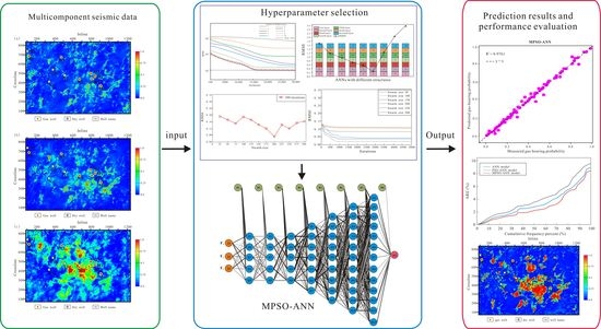
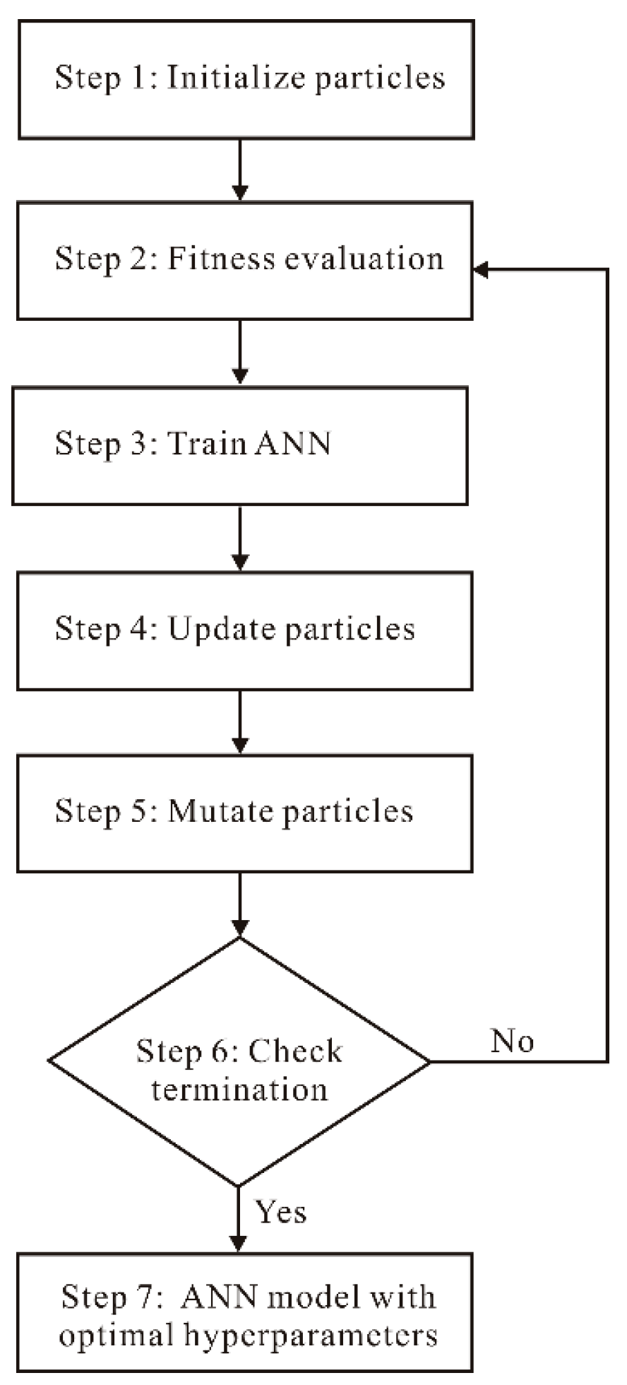
2.3. MPSO-ANN Framework

The MPSO-ANN model was obtained by using MPSO to optimize the weights and biases of the ANN model. The weights and biases were set as position vectors in the MPSO, and the root mean square error (RMSE) (Equation (5)) was used as the fitness function. After multiple iterations, the fitness reached the setting accuracy, and training ended, and the optimal result was obtained, as follows (Figure 2).

Step 1: Initialize the swarm size, inertial weight, velocity coefficients, maximum iterations, and velocity and position of each particle.

Step 2: Evaluate the fitness, and select the best position with the lowest fitness.

Step 3: For each candidate particle, train the ANN model with the corresponding parameters.

Step 4: Update the velocity and position of each particle according to Equations (1) and (2).

Step 5: If r(t) > 0.9, mutate the particles that satisfy the requirements according to Equation (3).

Step 6: Check the stop criteria. If the accuracy requirement is not satisfied, return to Step 2. Otherwise, iteration is stopped, and the optimal parameters are obtained.

Step 7: The obtained optimal results are assigned to the key parameters of the ANN.

2.4. Performance Evaluation of the Model

The model performance was evaluated using the mean square error (MSE), RMSE, and determination coefficient (R²), as shown in Equations (4)–(6).

$$\mathrm{MSE}=\frac{1}{n}{\displaystyle \sum _{i=1}^n{(y_{predicted}-y_{real})}^2}$$

(4)

$$\mathrm{RMSE}=\sqrt{\frac{1}{n}{\displaystyle \sum _{i=1}^n{(y_{predicted}-y_{real})}^2}}$$

(5)

$${\mathrm{R}}^2=1-\frac{{\displaystyle {\sum }_{i=1}^n{(y_{predict}-y_{real})}^2}}{{\displaystyle {\sum }_{i=1}^n{(\overline{y_{real}}-y_{real})}^2}}$$

(6)

where $y_{real}$ is the real value, $y_{predicted}$ is the predicted result, $\overline{y_{real}}$ is the average $y_{real}$, and n is the total number.

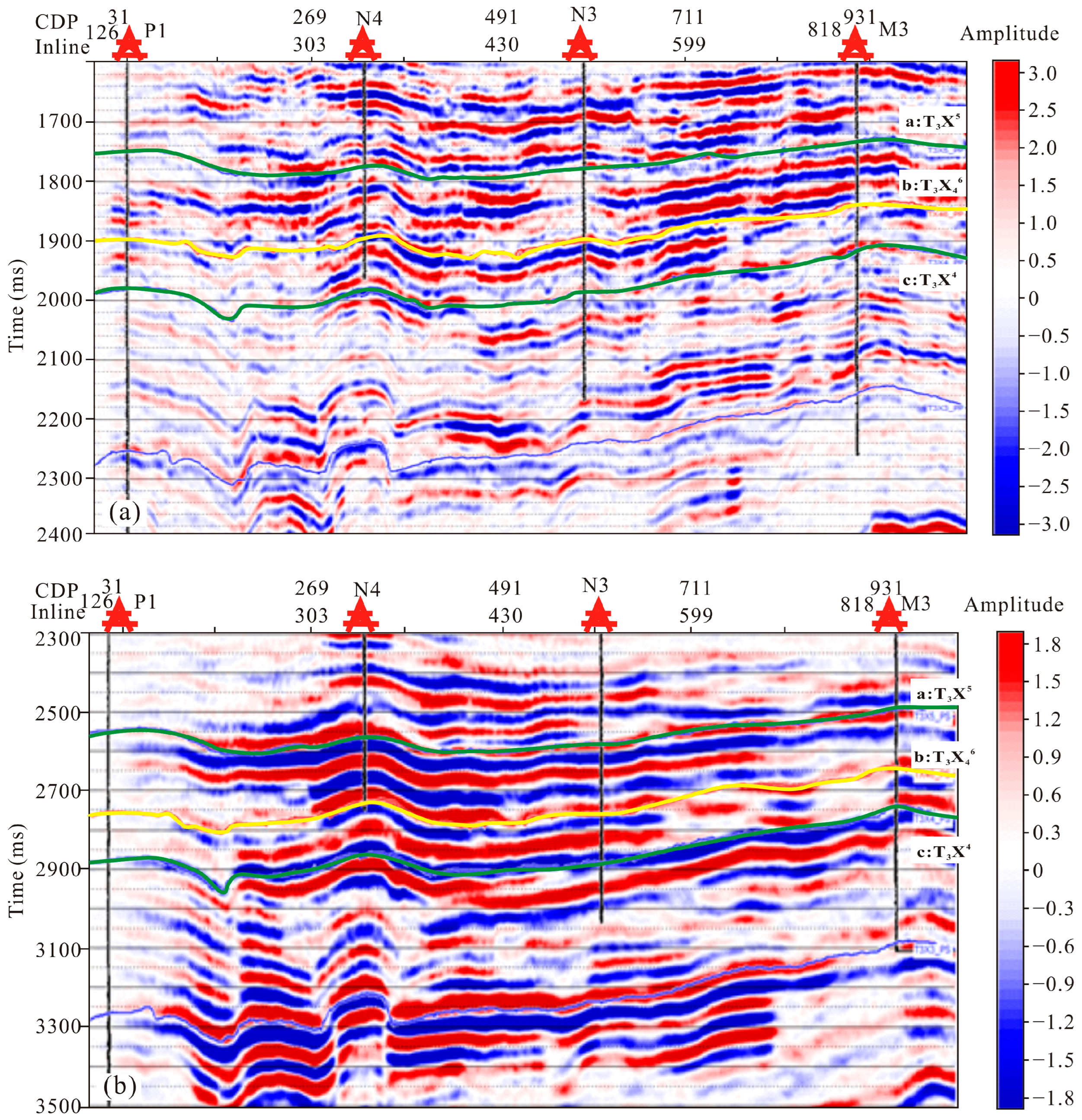
3. Study Area and Available Data

The multicomponent seismic data used in this study are from the Fenggu structural area in the Western Sichuan Depression (WSD) (Figure 3). The WSD has experienced multistage tectonic movement associated with the Indosinian, Yanshanian, and Himalayan events and has always represented a passive subsidence environment controlled by the uplift and compression of the surrounding mountain systems [44,45]. The deep Xujiahe Formation contains a rich gas reservoir, but its exploration and development are difficult, owing to its complex geological conditions, tight low-permeability sandstone, high heterogeneity, and abnormal ultrahigh fluid pressure [46].

Furthermore, the tight low-permeability sandstone of the Xujiahe Formation contains effective matrix pores and fractures, which control the distribution of natural gas and its enrichment and production, respectively. Multicomponent seismic exploration technology can effectively predict high-quality reservoirs, detect fractures, and identify gas-bearing horizons; thus, it is suitable for exploring tight sandstone gas reservoirs. The work areas of multicomponent seismic exploration and available drilling are shown in Figure 4. Figure 5 illustrates the horizon calibration results of the synthetic seismic record of well M3. Figure 6 shows the well-tie seismic profiles of P1, N4, N3, and M3, where T₃X₄⁶ is the target horizon.

Seismic attribute analysis has become an effective method for reservoir prediction [47,48]. Compared with the use of single longitudinal wave seismic attribute data, the comprehensive utilization of the sensitivity difference between the multicomponent seismic attributes as underground reservoir information is helpful in reducing the multi-resolution caused by single-component seismic attributes. However, it is challenging to extract hydrocarbon-sensitive features from multicomponent seismic attributes effectively. Unlike longitudinal wave seismic attributes, multicomponent seismic attribute data include converted shear wave attribute data, making it difficult to utilize these data to obtain effective gas reservoir information completely.

We optimized three composite attributes (F₁, F₂, F₃) (Figure 7) from the multicomponent seismic attributes for gas-bearing prediction. The detailed optimization process and constituent attributes of the three composite attributes are available in the literature [49]. These three composite attributes effectively extracted information on gas-sensitive characteristics and provided good data sources for the ANN. In addition, because of the complex relationship between seismic attributes and gas reservoirs, it is challenging to make full use of the complex nonlinear relationship between them to achieve accurate prediction. Therefore, in this study, three composite attributes consistent with a previous study were selected as the input to verify whether the proposed method can improve the prediction accuracy.

The gas-bearing probability was considered as the prediction output of the ANN model. It was obtained using a correlation calculation [50,51]. Finally, 230 sample points were obtained from 11 wells (Figure 4) as the sample dataset. The training and test datasets were divided into a 7:3 ratio. The sample dataset characteristics are shown in Figure 8, where the abscissa shows the sample value, and the ordinate shows the frequency probability. The attributes of F₁, F₂, and F₃ were mainly concentrated between 0 and 0.2, 0.2 and 0.6, and 0.4 and 0.8, respectively. This difference in the characteristics of the three attributes reflects the diversity of the sample dataset. The gas-bearing probability is between 0 and 1, in agreement with the actual situation of different wells.

4. Analysis and Design of MPSO-ANN Model Parameters

The MPSO-ANN model was designed in three steps. (1) The hyperparameters of the ANN were determined, and an ANN model with better gas-bearing probability prediction performance was obtained. (2) The initial parameters of the MPSO were determined. (3) The MPSO-ANN model was obtained by using the MPSO to optimize the developed ANN model.

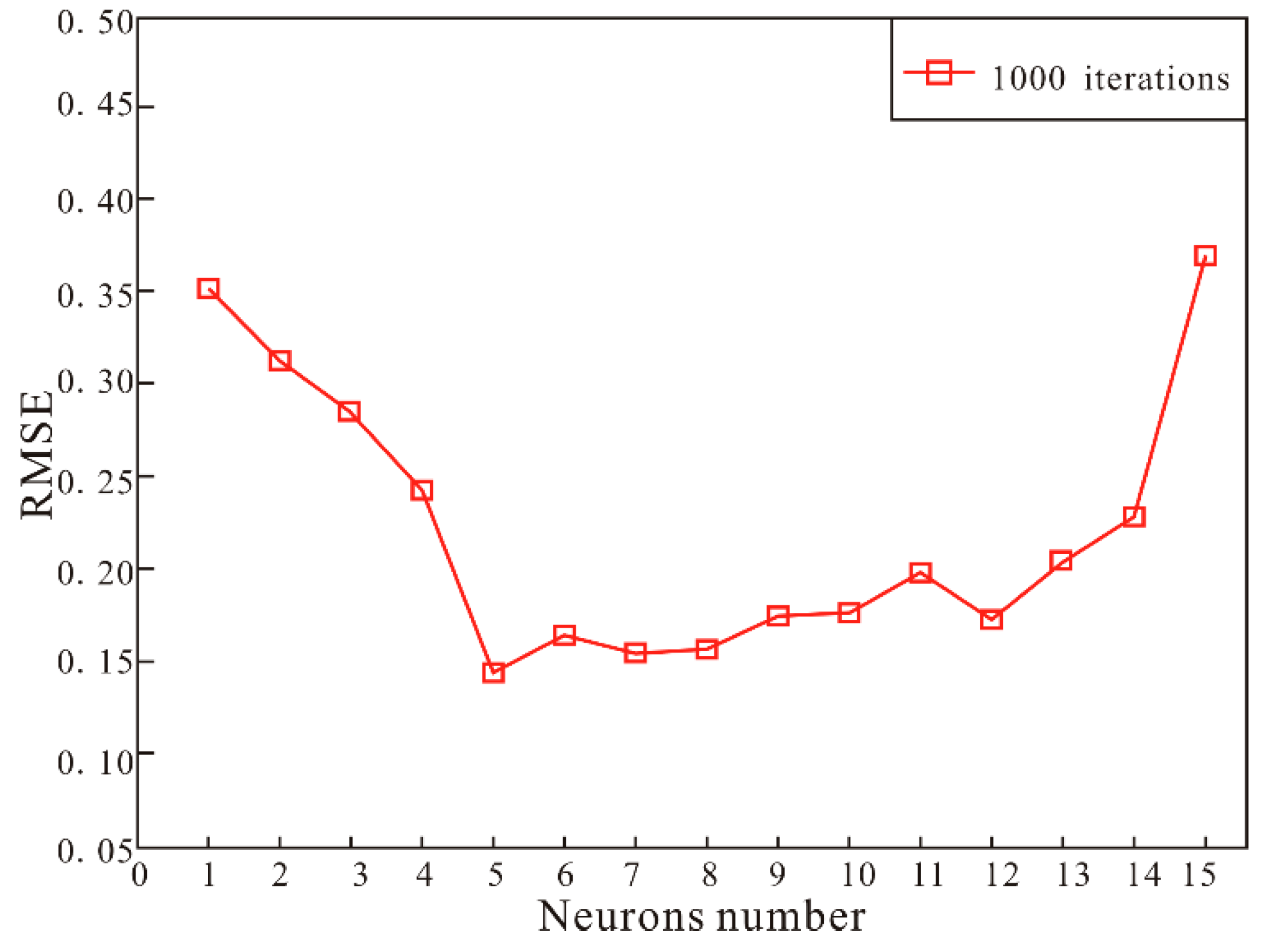
4.1. ANN Architecture

The ANN was designed by selecting the hyperparameters according to their effects on model performance; some affect the prediction accuracy, whereas others affect the computational efficiency. Hyperparameter selection is a complex process. The most challenging part of this process is determining the number of hidden layers and neurons (Figure 1). Their number is not fixed, and a larger number makes the network overfitted, resulting in low accuracy and increased computation time. A smaller number makes the network underfitted, resulting in reduced accuracy. Therefore, this study experimentally determined these numbers.

The training dataset was used to determine the optimal number of hidden layers and evaluate the gas-bearing prediction ability of ANNs with different numbers of hidden layers (Figure 9). At the beginning of network training, all the ANNs had large errors, which decreased as training progressed. The errors of network models with more hidden layers decreased rapidly, whereas those of models with fewer hidden layers decreased slowly. The fastest decrease in errors was observed for ANNs with 7–9 hidden layers, and the accuracy requirement was met at ~15,000 iterations. Further increases in iterations did not significantly change the errors of the three ANNs, and they remained stable. A slight increase in errors was observed for an ANN with 10 hidden layers, indicating the presence of too many hidden layers at this time, and the network was overfitted. Although the errors of ANN models with 8 and 9 hidden layers were slightly lower than that of a model with 7 hidden layers, the latter already met the target value requirements, with little difference depending on the iterations. Considering the duration, the optimal number was determined to be 7.

Next, we used the training dataset to analyze the prediction ability of networks with seven hidden layers and different numbers of neurons. It was determined by a trial-and-error method, and the model performance was evaluated using the RMSE. Figure 10 shows the errors for different numbers of neurons in the first hidden layer, which indicates that this characteristic significantly impacts the accuracy. When the number reached 15, the error became significant. When the number is five, the RMSE is the lowest; thus, the optimal number of neurons in the first hidden layer was determined to be five.

To determine the number of nodes in a hidden layer, those in other hidden layers were not changed. Figure 11 shows the process of error analysis used to determine the number of nodes in the seventh hidden layer. In this process, the number of nodes in the first six hidden layers (5, 5, 5, 7, 9, and 11) were unchanged, and only that in the seventh hidden layer was changed; the error of different models was then analyzed.

The network error increased significantly when the number of nodes exceeded 15, for example, when it was 17 and 19 (Figure 11), indicating a complex network structure and low accuracy. If the number of nodes is not carefully selected and the neural network structure for gas-bearing prediction is blindly determined, the prediction will not only be time-consuming but will also fail to yield the desired effect. The RMSE was the lowest with 13 nodes; thus, the number of neurons in the seventh hidden layer was determined to be 13. Finally, the number of hidden layers in the network was determined to be seven, and the numbers of neurons in the hidden layers were 5, 5, 5, 7, 9, 11, and 13.

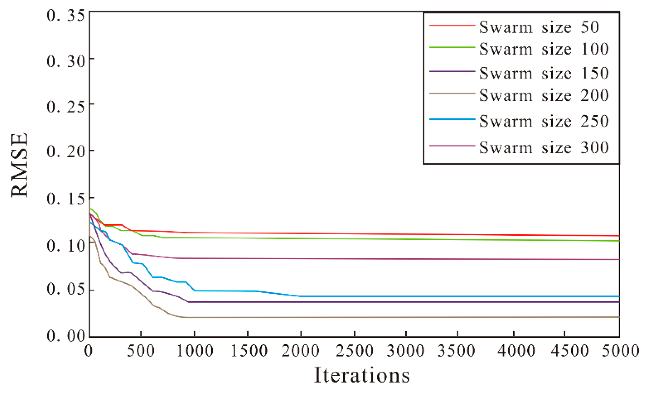
4.2. Design of MPSO Algorithm Parameters

After the initial ANN model was determined, the same network structure was followed as that in MPSO parameter selection, that is, (3-5-5-5-7-9-11-13-1). The precise selection of MPSO parameters is helpful for efficiently optimizing the ANN model and obtaining a model with good predictive performance for the gas-bearing probability. These MPSO parameters include the swarm size, velocity coefficients, and termination criteria. However, these parameters cannot be determined simultaneously. The control variable method was adopted to select parameters to obtain the optimal values.

First, the swarm size was selected. The velocity coefficients (C₁ = C₂ = 2) were fixed, and the inertia weight was set to 0.8. Figure 12 displays the RMSE of MPSO-ANN for different swarm sizes after 100 iterations. When the swarm size was relatively small (e.g., 25 and 50), the RMSE of the model was relatively large, indicating that a small swarm size cannot satisfy the accuracy requirements. However, even large swarm sizes (e.g., 275 and 300) showed large model errors and were time-consuming. The lowest RMSE was obtained at a swarm size of 200, indicating better prediction performance of the model. Therefore, the swarm size was set to 200.

Subsequently, the velocity coefficients C₁ and C₂ (Equation (1)) were studied. C₁ determines the local range of the searchability of the particles, and C₂ determines how quickly particles converge to the optimal value. C₁ = 2 and C₂ = 2 are often used in PSO studies, but these are not necessarily the best velocity coefficient values [52]. Here, the swarm size was set to 200, the inertial weight was 0.8, and iterations was 100.

Table 1. RMSE of different velocity coefficient (C₁ and C₂) combinations.

C1	C2	Combination of C1 and C2	RMSE	Rank
0.5	2.5	3	0.0686	6
1	2	3	0.7126	8
1.25	2.75	4	0.0642	3
1.5	2.5	4	0.0654	5
1.75	2.25	4	0.0606	1
2	2	4	0.0623	2
2	3	5	0.0692	7
2.5	2.5	5	0.0645	4

lists the C₁ and C₂ values and RMSE of various combinations. The velocity coefficient combination of C₁ = 1.75 and C₂ = 2.25 had the lowest RMSE; therefore, this coefficient combination was used in this study.

Finally, the termination conditions of the model were determined. Increasing the iterations reduced the error but increased the training time. When the model achieved a certain accuracy, its error became stable with training. In this case, continuing the training process did not significantly improve accuracy but increased the calculation cost. Therefore, this study determined the optimal number of iterations by comparing the RMSE. Figure 13 shows the RMSE with various numbers of iterations for different swarm sizes. The error decreased rapidly during the first 500 iterations, after which the RMSE of the model with a small swarm did not change, and the error was large. As training progressed, the error decreased slowly. When the number of iterations reached 1000, the error became stable, and the model error with a swarm size of 200 was low. Therefore, the number of iterations was set to 1000.

4.3. Determining the MPSO-ANN Model

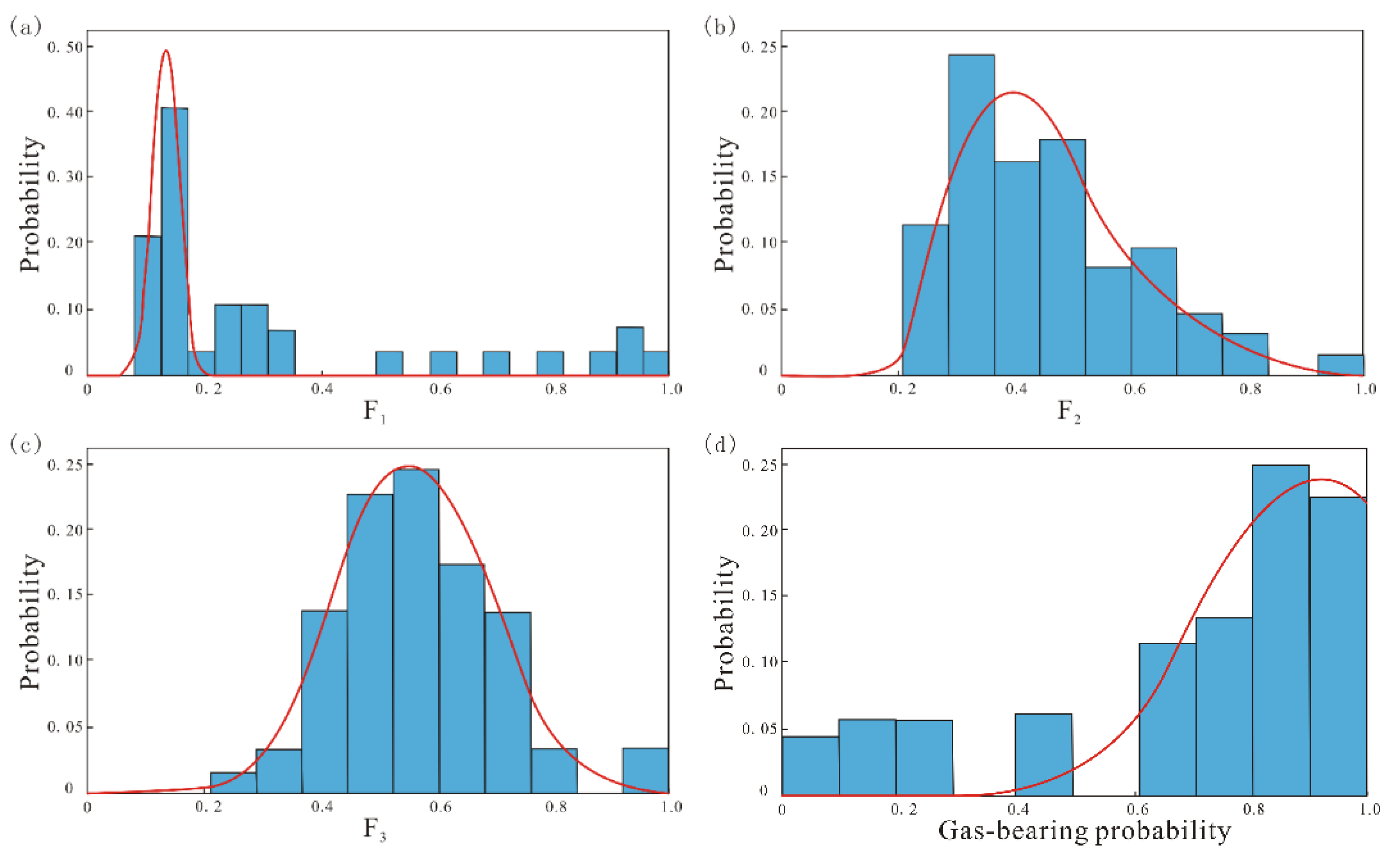
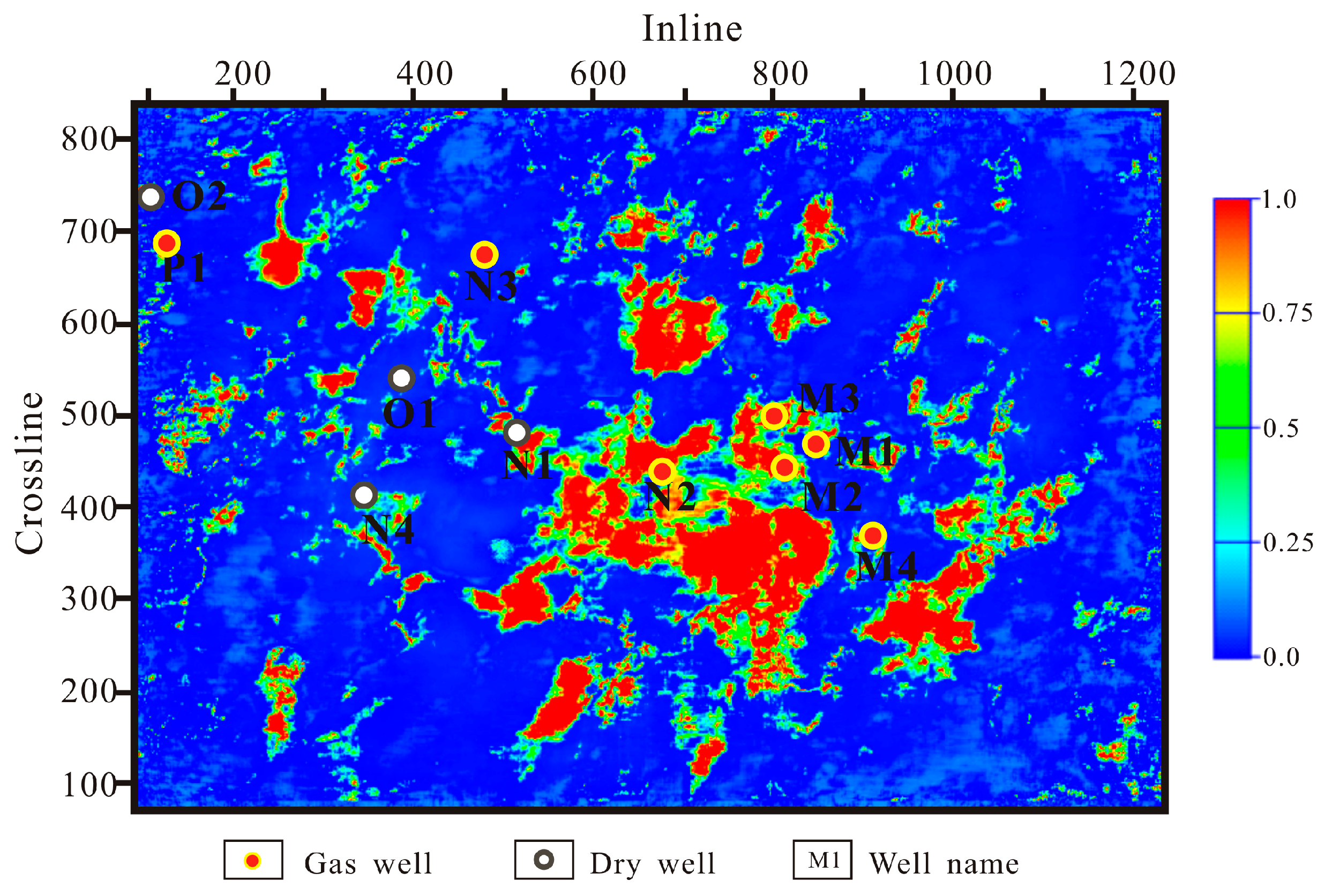
The MPSO-ANN model parameters were determined by designing the initial ANN model and selecting the MPSO algorithm parameters. The network structure was (3-5-5-5-7-9-11-13-1), swarm size was 200, velocity coefficients were C₁ = 1.75 and C₂ = 2.25, and maximum number of iterations was 1000.

The MPSO-ANN continuously adjusted its weights and biases during optimization (Figure 14) to gradually reduce the error. Finally, the MPSO-ANN model for gas-bearing distribution prediction was determined (Figure 15). Figure 16 shows the RMSE of MPSO-ANN, PSO-ANN, and ANN on the training dataset with increasing iterations. The three network models achieved a low MSE, but the optimization speed of MPSO was better than that of ANN. The error of ANN stabilized after ~15,000 iterations, whereas that of the MPSO stabilized after ~1000 iterations, and the error was lower in the latter, indicating that the MPSO-ANN model significantly outperformed the ANN model. The MPSO-ANN model also has fewer iterations and lower error than the PSO-ANN model (Figure 16), which shows that MPSO can optimize the ANN model more quickly and accurately.

5. Results

The determined neural network model (Figure 15) was applied to the test dataset, and the prediction result had a high fit (R² = 0.9761). In addition, the predicted gas-bearing probability of MPSO-ANN (Figure 17) is close to the ideal line (dotted black line), indicating that the predicted result is highly consistent with the measured result. Then, the MPSO-ANN model was used to predict the gas-bearing distribution of the target layer (Figure 18). The obtained results were validated using actual drilling data, which showed that four dry wells are predicted to be dry wells. Moreover, all gas wells (except for N3) are all predicted to be gas-bearing, in agreement with drilling information, and the gas-bearing distribution varied greatly. N3 was inaccurately predicted because even though it is a gas well, its gas content is lower than that of the others; thus, the obtained gas-bearing probability was lower, leading to differences in the prediction result.

To check the validity of the developed model, the prediction results of the MPSO-ANN, PSO-ANN, and ANN models (without optimization) were compared. The probability density function (PDF) of the error percentage of the three models on the test dataset was compared (Figure 19). The error of MPSO-ANN was small; specifically, the error of most MPSO-ANN data was the smallest (<5%), and there were no data with large errors (>10%). Moreover, the data points predicted by the MPSO-ANN model were more consistent with the actual results (i.e., the error was 0) than those of PSO-ANN and ANN models, indicating it has better prediction performance. To intuitively compare the prediction errors, Figure 20 shows the absolute relative error (ARE) of the three models on the test data. The AREs of the three models were <10%, indicating that no data points had particularly large errors. In ascending order, the error of the MPSO-ANN model was the smallest, followed by that of the PSO-ANN model and, finally, that of the ANN model. The error comparison of the three models shows that MPSO-ANN had higher prediction accuracy.

Further analysis of the performance indicators of the three models on the test dataset (

Table 2. Performance of different models for the test dataset.

Model	Performance Indicators
	MSE	RMSE	R2
ANN	0.0069	0.0833	0.9625
PSO-ANN	0.0062	0.0786	0.9713
MPSO-ANN	0.0058	0.0762	0.9761

) revealed that of the three models, the MPSO-ANN model has the lowest error (MSE = 0.0058, RMSE = 0.0762) and the best fit (R² = 0.9761). The PSO-ANN model has the next-highest error (MSE = 0.0062, RMSE = 0.0786) and the next-worst fit (R² = 0.9713), and the ANN model has the highest error (MSE = 0.0069, RMSE = 0.0833) and the worst fit (R² = 0.9625). Further comparison showed that the MSE and RMSE of MPSO-ANN were 6.45% and 3.05% smaller than those of PSO-ANN and 15.94% and 8.52% smaller than those of ANN, respectively. According to Figure 19 and Figure 20 and Table 2, MPSO-ANN shows better predictive performance on the test dataset. In addition, the performance of the three models on the training dataset (Figure 16) reveals that of the three models, MPSO-ANN required fewer iterations to stabilize more quickly and had lower errors in the training process. These results show that the MPSO-ANN model developed can achieve higher prediction accuracy with fewer iterations compared to the PSO-ANN and ANN models, verifying the effectiveness of the MPSO-ANN model.

Moreover, we also compared the predicted results across the entire area using the three models (Figure 21). The prediction result of the PSO-ANN model (Figure 21b) was consistent overall with that of the MPSO-ANN model (Figure 18), and both were relatively accurate. However, the predicted gas-bearing probability of the former was slightly lower than that of the latter (Figure 18), which is consistent with the AREs (Figure 20). The gas reservoir distribution boundary output by the ANN model (Figure 21a) was fuzzy, and some gas-bearing probabilities were observed for the dry wells O2 and N4, which were inconsistent with the real data (i.e., 0). Therefore, the ANN had a higher error than MPSO-ANN and PSO-ANN. This analysis further verifies the effectiveness of the developed model.

6. Discussion

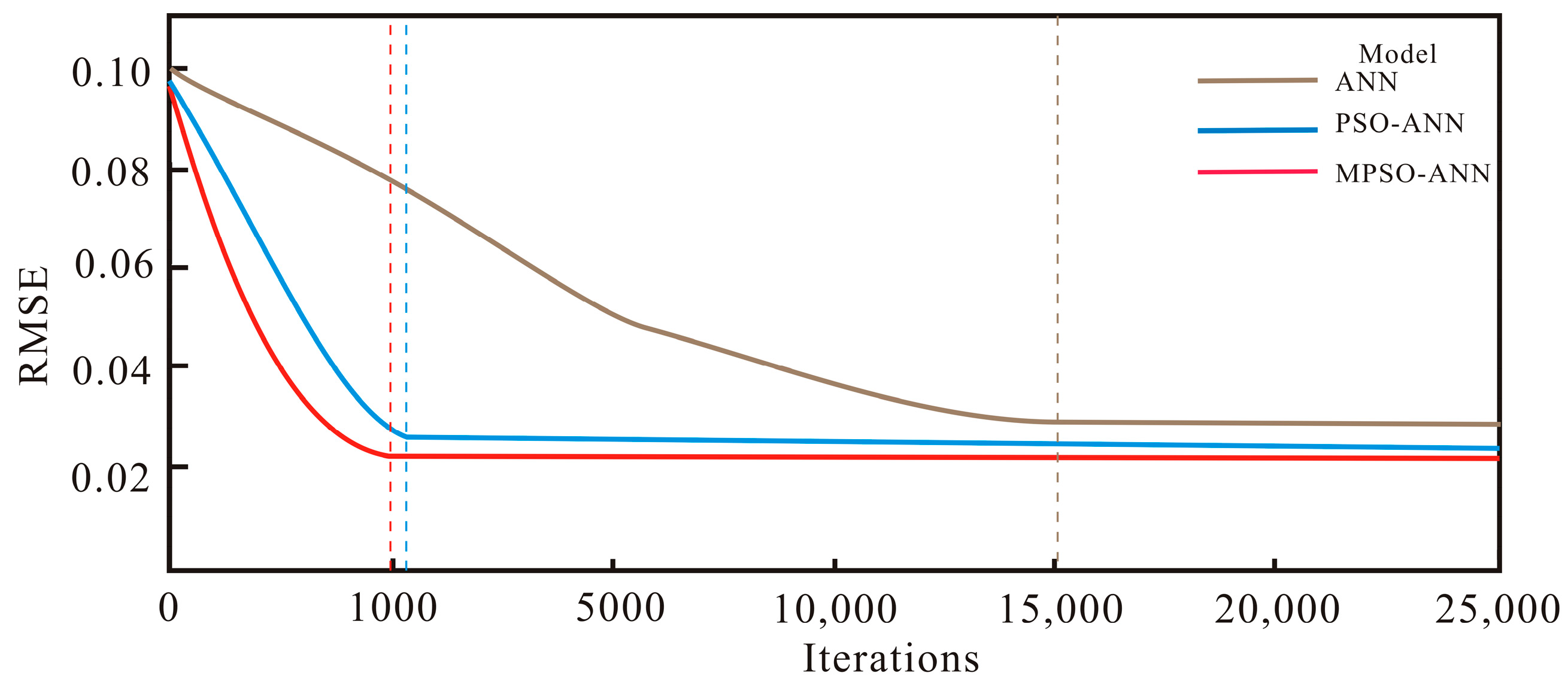
6.1. Comparison with ANN Training Algorithms

To evaluate the performance of MPSO-ANN, we compared it with commonly used training algorithms. Figure 22 shows the iterations required by different algorithms to satisfy the preset error (i.e., MSE < 0.001) on the training dataset. Many training algorithms are used to adjust the weights and biases of ANNs [53], such as the gradient descent and Newton methods. The gradient descent method is simple and convenient, but its convergence speed is slow, and it easily falls into local minima. The Newton method converges more rapidly than the gradient descent method, but the calculation process is complex, and the calculation cost is high [29]. The LMA is a comprehensive algorithm combining the fastest descent and Gauss–Newton methods. It combines the advantages of the gradient descent and Newton methods by combining coefficients, significantly reducing the occurrence of local minimum problems and improving computational efficiency [54]. Therefore, among these training algorithms (except for the MPSO algorithm), the LMA uses fewer iterations to satisfy the preset error.

However, the MPSO-ANN model met the error requirement in less than 1000 iterations, whereas the LMA that decreased the fastest compared to other training algorithms (except MPSO) did not meet the error requirement until ~15,000 iterations. The reason is that, compared with the other training algorithms, PSO could carefully search for the global optimal solution without relying on the gradient of the target or any differential form. Therefore, it has the advantages of easy implementation and fast convergence while ensuring high prediction accuracy. In addition, this study decreases the diversity loss caused by the excessive concentration of particles by adding the particle mutation operation to the PSO and alleviates the problem of falling into the local optimal solution, which gives the MPSO algorithm clear advantages over these training algorithms. This analysis suggests that the MPSO-ANN model has a better search ability than other algorithms.

Figure 23 shows the RMSE and R² values of different algorithms on the test dataset. The ANN model optimized with MPSO (MPSO-ANN) showed the lowest RMSE and highest R², indicating better prediction results than those of the ANN model obtained with the above training algorithm. Furthermore, a comparison of different algorithms on the training dataset (Figure 22) showed that some optimization algorithms (e.g., SGD) required more iterations during model development but had larger errors on the test dataset. Thus, these algorithms cannot efficiently optimize the weights and biases, resulting in inaccurate information transfer between them. Among them, the MPSO algorithm required the fewest iterations in ANN model development (i.e., MPSO-ANN) and had the highest accuracy on the test dataset, indicating that it provides a powerful search and optimization scheme for determining the weights and biases of the ANN.

6.2. Comparison with Single-Component Seismic Data

To verify the influence of multicomponent seismic data on the prediction results of the MPSO-ANN model, we analyzed the prediction results obtained using only single-component seismic attributes as input data. The obtained prediction results (Figure 24) were not consistent with the drilling data; thus, it was inferred that good prediction results could not be obtained using single-component data. Compared with the multicomponent seismic gas-bearing prediction results of MPSO-ANN (Figure 18), the gas reservoir boundary obtained by single-component seismic gas-bearing prediction using MPSO-ANN was fuzzy, and the accuracy was low.

The study area was a tight sandstone gas reservoir with complex seismic response characteristics. Sample data can be obtained by using the response of multicomponent seismic attributes to gas reservoirs, from which sensitive information on the gas reservoir can be extracted to provide high-quality samples for ANN model and improve prediction accuracy. The input data significantly impacted the prediction ability of MPSO-ANN. Multicomponent seismic data can provide good information for MPSO-ANN prediction. However, the use of good data sources alone is insufficient. For example, an unoptimized ANN can also be used for gas-bearing prediction (Figure 21a); however, the prediction results have a large error. Not only is good data information needed to predict unconventional reservoirs, but network models with good predictive performance are also required to learn the data characteristics. Therefore, the proposed MPSO-ANN model meets this requirement well and achieves good prediction results.

6.3. Application to Other Datasets

The above research verifies the validity of the MPSO-ANN model constructed in this study through a case study. There are differences in the real data available for gas-bearing prediction applications in different regions, and it is impossible to test the validity of the MPSO-ANN model on all real datasets. Therefore, to further verify the effectiveness and generalizability of the constructed MPSO-ANN model, we applied it to a synthetic dataset for gas-bearing distribution prediction. To increase the universality of the numerical model, the structure of the numerical model is obtained from the Marmousi2 model [55], which has been widely used in the testing of seismic inversion, imaging, and other methods. In addition, the Marmousi2 model itself contains reservoir information, which is very suitable for testing reservoir prediction methods. Figure 25a shows part of the Marmousi2 model, which includes a gas reservoir (blue area). We obtained the seismic records of longitudinal wave and converted shear wave by wave equation forward modeling, and obtained the composite attributes through composite operations [49] to construct the sample dataset. During the label making process, we selected three seismic traces as pseudo-wells (as shown by the white dotted line in Figure 25b). The gas reservoir and non-gas reservoir characteristics were marked on the data of the pseudo-well seismic traces, and labels were made.

The ANN, PSO-ANN, and MPSO-ANN models were applied to the synthetic data for training and prediction, and the obtained results are shown in Figure 26. The prediction error was obtained by comparing the predicted results with the actual gas reservoir distribution. Among the three models, the ANN model has the largest error, followed by the PSO-ANN model, and the MPSO-ANN model has a smaller error, indicating that the prediction results of the MPSO-ANN model are more consistent with the actual gas reservoir. The effectiveness of the model is further verified by the synthetic data.

In this study, we verified the effectiveness of the developed MPSO-ANN model using a case study and a universal numerical model. In future work, we will consider testing in more regions or datasets to verify its generalizability further. In general, the results of this study apply not only to the gas-bearing distribution but also to other problems, such as optimizing the hyperparameters of conventional ML models [56] and deep learning models [57]. This study can provide a reference for the parameter setting of the PSO algorithm. In addition, when applying ANNs to other prediction problems, such as slope stability identification using remote sensing images [58] and smallholder irrigated agriculture mapping using remote sensing techniques [59], the results of this study can be used to set the hyperparameters of the ANN model in a targeted way to reduce computing costs. The results of this study provide a reference for the parameter setting of PSO and ANNs in other applications.

7. Conclusions

A new method for predicting the gas-bearing distribution of unconventional reservoirs was proposed using an MPSO-ANN model with multicomponent seismic data, and a prediction model with high prediction accuracy was established by carefully evaluating the MPSO-ANN parameters. The results indicate that the optimization ability of the MPSO-ANN model is much better than that of PSO-ANN and ANN models. Moreover, the MPSO-ANN model met the error requirement (MSE < 0.001) in less than 1000 iterations, whereas the LMA that decreased the fastest among other conventional training algorithms (except MPSO) did not meet the error requirement until ~15,000 iterations. These results suggest that MPSO can achieve a low RMSE and high R² in only a few iterations, providing a powerful search and optimization scheme for determining the weights and biases of the ANN.

In general, the research results could contribute to the application of ANNs in unconventional reservoir prediction and also have reference significance for the application of PSO and ANNs in other fields. Inevitably, the method developed in this study also has some limitations. This study applies the mutation operation in the PSO algorithm to address the lack of diversity caused by the excessive concentration of particles. However, the inertia weight and velocity coefficients of the PSO algorithm also affect its searchability. In future work, attempts may be made to automatically adjust them during training to alleviate local optimization problems effectively. Additionally, in our subsequent work, we will consider testing the MPSO-ANN model in more regions or datasets to validate its generalizability and effectiveness further.

References

1. Hui, G.; Chen, S.N.; He, Y.M.; Wang, H.; Gu, F. Machine learning-based production forecast for shale gas in unconventional reservoirs via integration of geological and operational factors. J. Nat. Gas Sci. Eng. 2021, 94, 104045. [Google Scholar] [CrossRef]
2. Pan, Y.W.; Deng, L.C.; Zhou, P.; Lee, W.J. Laplacian Echo-State Networks for production analysis and forecasting in unconventional reservoirs. J. Pet. Sci. Eng. 2021, 207, 109068. [Google Scholar] [CrossRef]
3. Yang, J.Q.; Lin, N.T.; Zhang, K.; Fu, C.; Cui, Y.; Li, G.H. An Improved Small-Sample Method Based on APSO-LSSVM for Gas-Bearing Probability Distribution Prediction From Multicomponent Seismic Data. IEEE Geosci. Remote S. 2023, 20, 7501705. [Google Scholar] [CrossRef]
4. Park, J.; Datta-Gupta, A.; Singh, A.; Sankaran, S. Hybrid physics and data-driven modeling for unconventional field development and its application to US onshore basin. J. Pet. Sci. Eng. 2021, 15, 109008. [Google Scholar] [CrossRef]
5. Cao, J.X.; Jiang, X.D.; Xue, Y.J.; Tian, R.F.; Xiang, T.; Cheng, M. The State-of-the-Art Techniques of Hydrocarbon Detection and Its Application in Ultra-Deep Carbonate Reservoir Characterization in the Sichuan Basin, China. Front. Earth Sci. 2022, 10, 851828. [Google Scholar] [CrossRef]
6. Sun, J.; Innanen, K.A.; Huang, C. Physics-guided deep learning for seismic inversion with hybrid training and uncertainty analysis. Geophysics 2021, 86, R303–R317. [Google Scholar] [CrossRef]
7. Sun, J.; Niu, Z.; Innanen, K.A.; Li, J.X.; Trad, D.O. A theory-guided deep-learning formulation and optimization of seismic waveform inversion. Geophysics 2020, 85, R87–R99. [Google Scholar] [CrossRef]
8. Wang, H.; Chen, Z.; Chen, S.N.; Hui, G.; Kong, B. Production Forecast and Optimization for Parent-Child Well Pattern in Unconventional Reservoirs. J. Pet. Sci. Eng. 2021, 203, 108899. [Google Scholar] [CrossRef]
9. Zargar, G.; Tanha, A.A.; Parizad, A.; Amouri, M.; Bagheri, H. Reservoir rock properties estimation based on conventional and NMR log data using ANN-Cuckoo: A case study in one of super fields in Iran southwest. Petroleum 2020, 6, 304–310. [Google Scholar] [CrossRef]
10. Kalam, S.; Yousuf, U.; Abu-Khamsin, S.A.; Waheed, U.B.; Khan, R.A. An ANN model to predict oil recovery from a 5-spot waterflood of a heterogeneous reservoir. J. Pet. Sci. Eng. 2022, 210, 110012. [Google Scholar] [CrossRef]
11. Baziar, S.; Shahripour, H.B.; Tadayoni, M.; Nabi-Bidhendi, M. Prediction of water saturation in a tight gas sandstone reservoir by using four intelligent methods: A comparative study. Neural Comput. Appl. 2018, 30, 1171–1185. [Google Scholar] [CrossRef]
12. Jahan, L.N.; Munshi, T.A.; Sutradhor, S.S.; Hashan, M. A comparative study of empirical, statistical, and soft computing methods coupled with feature ranking for the prediction of water saturation in a heterogeneous oil reservoir. Acta Geophys. 2021, 69, 1697–1715. [Google Scholar] [CrossRef]
13. Liu, J.J.; Liu, J.C. An intelligent approach for reservoir quality evaluation in tight sandstone reservoir using gradient boosting decision tree algorithm—A case study of the Yanchang Formation, mid-eastern Ordos Basin, China. Mar. Pet. Geol. 2021, 126, 104939. [Google Scholar] [CrossRef]
14. Agbadze, O.K.; Cao, Q.; Ye, J.R. Acoustic impedance and lithology-based reservoir porosity analysis using predictive machine learning algorithms. J. Pet. Sci. Eng. 2022, 208, 109656. [Google Scholar] [CrossRef]
15. Kang, B.; Choe, J. Uncertainty quantification of channel reservoirs assisted by cluster analysis and deep convolutional generative adversarial networks. J. Pet. Sci. Eng. 2020, 187, 106742. [Google Scholar] [CrossRef]
16. Chen, L.F.; Guo, H.X.; Gong, P.S.; Yang, Y.Y.; Zuo, Z.L.; Gu, M.Y. Landslide susceptibility assessment using weights-of-evidence model and cluster analysis along the highways in the Hubei section of the Three Gorges Reservoir Area. Comput. Geosci. 2021, 156, 104899. [Google Scholar] [CrossRef]
17. Fu, C.; Lin, N.T.; Zhang, D.; Wen, B.; Wei, Q.Q.; Zhang, K. Prediction of reservoirs using multi-component seismic data and the deep learning method. Chin. J. Geophys. 2018, 61, 293–303. [Google Scholar]
18. Yasin, O.; Ding, Y.; Baklouti, S.; Boateng, C.D.; Du, Q.Z.; Golsanami, N. An integrated fracture parameter prediction and characterization method in deeply-buried carbonate reservoirs based on deep neural network. J. Pet. Sci. Eng. 2022, 208, 109346. [Google Scholar] [CrossRef]
19. Saikia, P.; Baruah, R.D.; Singh, S.K.; Chaudhuri, P.K. Artificial neural networks in the domain of reservoir characterization: A review from shallow to deep models. Comput. Geosci. 2020, 135, 104357. [Google Scholar] [CrossRef]
20. Luo, S.Y.; Xu, T.J.; Wei, S.J. Prediction method and application of shale reservoirs core gas content based on machine learning. J. Appl. Phys. 2022, 204, 104741. [Google Scholar] [CrossRef]
21. Yang, J.Q.; Lin, N.T.; Zhang, K.; Ding, R.W.; Jin, Z.W.; Wang, D.Y. A data-driven workflow based on multisource transfer machine learning for gas-bearing probability distribution prediction: A case study. Geophysics 2023, 88, B163–B177. [Google Scholar] [CrossRef]
22. Grana, D.; Azevedo, L.; Liu, M. A comparison of deep machine learning and Monte Carlo methods for facies classification from seismic data. Geophysics 2019, 85, WA41–WA52. [Google Scholar] [CrossRef]
23. Wang, J.; Cao, J.X. Data-driven S-wave velocity prediction method via a deep-learning-based deep convolutional gated recurrent unit fusion network. Geophysics 2021, 86, M185–M196. [Google Scholar] [CrossRef]
24. Yang, J.Q.; Lin, N.T.; Zhang, K.; Zhang, C.; Fu, C.; Tian, G.P.; Song, C.Y. Reservoir Characterization Using Multi-component Seismic Data in a Novel Hybrid Model Based on Clustering and Deep Neural Network. Nat. Resour. Res. 2021, 30, 3429–3454. [Google Scholar] [CrossRef]
25. Song, Z.H.; Yuan, S.Y.; Li, Z.M.; Wang, S.X. KNN-based gas-bearing prediction using local waveform similarity gas-indication attribute—An application to a tight sandstone reservoir. Interpretation 2022, 10, SA25–SA33. [Google Scholar] [CrossRef]
26. Wang, J.; Cao, J.X.; Yuan, S. Deep learning reservoir porosity prediction method based on a spatiotemporal convolution bi-directional long short-term memory neural network model. Geomech. Energy Environ. 2021, 32, 100282. [Google Scholar] [CrossRef]
27. Zheng, D.Y.; Wu, S.X.; Hou, M.C. Fully connected deep network: An improved method to predict TOC of shale reservoirs from well logs. Mar. Petrol. Geol. 2021, 132, 105205. [Google Scholar] [CrossRef]
28. Mohaghegh, S.; Arefi, R.; Ameri, S.; Rose, D. Design and development of an artificial neural network for estimation of formation permeability. SPE Comput. Appl. 1995, 7, 151–154. [Google Scholar] [CrossRef]
29. Brantson, E.T.; Ju, B.S.; Ziggah, Y.Y.; Akwensi, P.H.; Sun, Y.; Wu, D.; Addo, B.J. Forecasting of Horizontal Gas Well Production Decline in Unconventional Reservoirs using Productivity, Soft Computing and Swarm Intelligence Models. Nat. Resour. Res. 2019, 28, 717–756. [Google Scholar] [CrossRef]
30. Keyvani, F.; Amani, M.J.; Kalantariasl, A.; Vahdani, H. Assessment of Empirical Pressure–Volume–Temperature Correlations in Gas Condensate Reservoir Fluids: Case Studies. Nat. Resour. Res. 2020, 29, 1857–1874. [Google Scholar] [CrossRef]
31. Saboori, M.; Homayouni, S.; Hosseini, R.S.; Zhang, Y. Optimum Feature and Classifier Selection for Accurate Urban Land Use/Cover Mapping from Very High Resolution Satellite Imagery. Remote Sens. 2022, 14, 2097. [Google Scholar] [CrossRef]
32. Ebtehaj, I.; Bonakdari, H.; Zaji, A.H.; Gharabaghi, B. Evolutionary optimization of neural network to predict sediment transport without sedimentation. Complex Intell. Syst. 2021, 7, 401–416. [Google Scholar] [CrossRef]
33. Mohamadi-Baghmolaei, M.; Sakhaei, Z.; Azin, R.; Osfouri, S.; Zendehboudim, S.; Shiri, H.; Duan, X.L. Modeling of well productivity enhancement in a gas-condensate reservoir through wettability alteration: A comparison between smart optimization strategies. J. Nat. Gas Sci. Eng. 2021, 94, 104059. [Google Scholar] [CrossRef]
34. Sadowski, L.; Nikoo, M. Corrosion current density prediction in reinforced concrete by imperialist competitive algorithm. Neural Comput. Appl. 2014, 25, 1627–1638. [Google Scholar] [CrossRef] [PubMed] [Green Version]
35. Amiri, M.; Ghiasi-Freez, J.; Golkar, B.; Hatampour, A. Improving water saturation estimation in a tight shaly sandstone reservoir using artificial neural network optimized by imperialist competitive algorithm—A case study. J. Pet. Sci. Eng. 2015, 127, 347–358. [Google Scholar] [CrossRef]
36. Ouadfeul, S.A.; Aliouane, L. Total Organic Carbon Prediction in Shale Gas Reservoirs from Well Logs Data Using the Multilayer Perceptron Neural Network with Levenberg Marquardt Training Algorithm: Application to Barnett Shale. Arab. J. Sci. Eng. 2015, 40, 3345–3349. [Google Scholar] [CrossRef]
37. Chanda, S.; Singh, R.P. Prediction of gas production potential and hydrological properties of a methane hydrate reservoir using ANN-GA based framework. Therm. Sci. Eng. Prog. 2019, 11, 380–391. [Google Scholar] [CrossRef]
38. Mahmoodpour, S.; Kamari, E.; Esfahani, M.R.; Mehr, A.K. Prediction of cementation factor for low-permeability Iranian carbonate reservoirs using particle swarm optimization-artificial neural network model and genetic programming algorithm. J. Pet. Sci. Eng. 2021, 197, 108102. [Google Scholar] [CrossRef]
39. Mcculloch, W.S.; Pitts, W. A logical calculus of the ideas immanent in nervous activity. Bull. Math. Biol. 1943, 5, 115–133. [Google Scholar] [CrossRef]
40. Mehrjardi, R.T.; Emadi, M.; Cherati, A.; Heung, B.; Mosavi, A.; Scholten, T. Bio-Inspired Hybridization of Artificial Neural Networks: An Application for Mapping the Spatial Distribution of Soil Texture Fractions. Remote Sens. 2021, 13, 1025. [Google Scholar] [CrossRef]
41. Othman, A.; Fathy, M.; Mohamed, I.A. Application of Artificial Neural Network in seismic reservoir characterization: A case study from Offshore Nile Delta. Earth Sci. Inform. 2021, 14, 669–676. [Google Scholar] [CrossRef]
42. Eberhart, R.; Kennedy, J. A new optimizer using particle swarm theory. In MHS95, Proceedings of the Sixth International Symposium on Micro Machine and Human Science, Nagoya, Japan, 4–6 October 1995; IEEE: Piscataway, NJ, USA, 1995; pp. 39–43. [Google Scholar]
43. Kalantar, B.; Ueda, N.; Saeidi, V.; Janizadeh, S.; Shabani, F.; Ahmadi, K.; Shabani, F. Deep Neural Network Utilizing Remote Sensing Datasets for Flood Hazard Susceptibility Mapping in Brisbane, Australia. Remote Sens. 2021, 13, 2638. [Google Scholar] [CrossRef]
44. Lai, J.; Wang, G.W.; Fan, Z.Y.; Chen, J.; Wang, S.C.; Fan, X.Q. Sedimentary characterization of a braided delta using well logs: The Upper Triassic Xujiahe Formation in Central Sichuan Basin, China. J. Pet. Sci. Eng. 2017, 154, 172–193. [Google Scholar] [CrossRef]
45. Zhang, G.Z.; Yang, R.; Zhou, Y.; Li, L.; Du, B.Y. Seismic fracture characterization in tight sand reservoirs: A case study of the Xujiahe Formation, Sichuan Basin, China. J. Appl. Phys. 2022, 203, 104690. [Google Scholar] [CrossRef]
46. Zhang, K.; Lin, N.T.; Yang, J.Q.; Jin, Z.W.; Li, G.H.; Ding, R.W. Predicting gas bearing distribution using DNN based on multi-component seismic data: A reservoir quality evaluation using structural and fracture evaluation factors. Petrol. Sci. 2022, 19, 1566–1581. [Google Scholar] [CrossRef]
47. Hossain, S. Application of seismic attribute analysis in fluvial seismic geomorphology. J. Pet. Explor, Prod. Technol. 2020, 10, 1009–1019. [Google Scholar] [CrossRef] [Green Version]
48. Zhang, K.; Lin, N.T.; Yang, J.Q.; Zhang, D.; Cui, Y.; Jin, Z.W. An intelligent approach for gas reservoir identification and structural evaluation by ANN and Viterbi algorithm—A case study from the Xujiahe Formation, Western Sichuan Depression, China. IEEE Trans. Geosci. Remote Sens. 2023, 61, 5904412. [Google Scholar] [CrossRef]
49. Zhang, K.; Lin, N.T.; Fu, C.; Zhang, D.; Jin, X.; Zhang, C. Reservoir characterization method with multi-component seismic data by unsupervised learning and colour feature blending. Explor. Geophys. 2019, 50, 269–280. [Google Scholar] [CrossRef]
50. Lin, N.T.; Zhang, D.; Zhang, K.; Wang, S.J.; Fu, C.; Zhang, J.B. Predicting distribution of hydrocarbon reservoirs with seismic data based on learning of the small-sample convolution neural network. Chin. J. Geophys. 2018, 61, 4110–4125. [Google Scholar]
51. Gao, J.H.; Song, Z.H.; Gui, J.Y.; Yuan, S.Y. Gas-Bearing Prediction Using Transfer Learning and CNNs: An Application to a Deep Tight Dolomite Reservoir. IEEE Geosci. Remote Sens. Lett. 2020, 99, 1–5. [Google Scholar] [CrossRef]
52. Yagiz, S.; Karahan, H. Prediction of hard rock TBM penetration rate using particle swarm optimization. Int. J. Rock Mech. Min. Sci. 2011, 48, 427–433. [Google Scholar] [CrossRef]
53. Bishop, C.M. Neural Networks for Pattern Recognition; Oxford University Press: Oxford, UK, 1995. [Google Scholar]
54. Reynaldi, A.; Lukas, S.; Margaretha, H. Backpropagation and Levenberg–Marquardt algorithm for training finite element neural network. In Proceedings of the 2012 Sixth UKSim/AMSS European Symposium on Computer Modeling and Simulation (EMS), Valletta, Malta, 14–16 November 2012; IEEE: Piscataway, NJ, USA, 2012; pp. 89–94. [Google Scholar]
55. Martin, G.S.; Wiley, R.; Marfurt, K.J. Marmousi2: An elastic upgrade for Marmousi. Lead. Edge 2006, 25, 113–224. [Google Scholar] [CrossRef]
56. Chen, W.; Chen, Y.Z.; Tsangaratos, P.; Ilia, I.; Wang, X.J. Combining Evolutionary Algorithms and Machine Learning Models in Landslide Susceptibility Assessments. Remote Sens. 2020, 12, 3854. [Google Scholar] [CrossRef]
57. Wang, J.; Cao, J.X.; Yuan, S. Shear wave velocity prediction based on adaptive particle swarm optimization optimized recurrent neural network. J. Petrol. Sci. Eng. 2020, 194, 107466. [Google Scholar] [CrossRef]
58. Qian, L.H.; Zang, S.Y.; Man, H.R.; Sun, L.; Wu, X.W. Determination of the Stability of a High and Steep Highway Slope in a Basalt Area Based on Iron Staining Anomalies. Remote Sens. 2023, 15, 3021. [Google Scholar] [CrossRef]
59. Weitkamp, T.; Karimi, P. Evaluating the Effect of Training Data Size and Composition on the Accuracy of Smallholder Irrigated Agriculture Mapping in Mozambique Using Remote Sensing and Machine Learning Algorithms. Remote Sens. 2023, 15, 3017. [Google Scholar] [CrossRef]
Figure 1. Schematic of ANN structure.
Remotesensing 15 03987 g001
Figure 2. Flowchart of MPSO-optimized ANN.
Remotesensing 15 03987 g002
Figure 3. Location of the study area. The blue rectangle represents the Fenggu structural area.
Remotesensing 15 03987 g003
Figure 4. Acquisition work area and drilling distribution. There are 11 wells in the study area (7 gas wells and 4 dry wells). (Dotted line indicates the profiles of the connecting wells; it corresponds to the seismic profiles in Figure 6).
Remotesensing 15 03987 g004
Figure 5. Horizon calibration by logging curve in well M3: (a) longitudinal wave and (b) converted shear wave horizon calibration results. The synthetic seismic record corresponds to side-seismic data, showing that the well calibration results meet the requirements. Note: T3X4 and T3X5 represent the fourth and fifth members of the Xujiahe Formation, respectively, and the target is the sixth sand layer of the fourth member of the Xujiahe Formation.
Remotesensing 15 03987 g005
Figure 6. Well-tie seismic profiles of P1, N4, N3, and M3 (the red dotted line in Figure 4): (a) longitudinal wave and (b) converted shear wave well-tie seismic profiles. The green line represents the top and bottom of the fourth member of the Xujiahe Formation, and the yellow line represents the target layer, T3X46.
Remotesensing 15 03987 g006
Figure 7. Composite attributes: (a) F1, (b) F2, (c) F3.
Remotesensing 15 03987 g007
Figure 8. Sample data characteristics: (a) F1, (b) F2, (c) F3, and (d) gas-bearing probability.
Remotesensing 15 03987 g008
Figure 9. Performance of ANN with different numbers of hidden layers.
Remotesensing 15 03987 g009
Figure 10. Performance of ANNs with different numbers of neurons in the first hidden layer.
Remotesensing 15 03987 g010
Figure 11. Performance of ANNs with different numbers of neurons in the seventh hidden layer.
Remotesensing 15 03987 g011
Figure 12. Performance of MPSO-ANNs with different swarm sizes.
Remotesensing 15 03987 g012
Figure 13. Performance of MPSO-ANNs with different iterations.
Remotesensing 15 03987 g013
Figure 14. Proposed MPSO-ANN model for gas-bearing distribution prediction.
Remotesensing 15 03987 g014
Figure 15. Structure of proposed MPSO-ANN model (after optimization) for gas-bearing distribution prediction.
Remotesensing 15 03987 g015
Figure 16. Comparison of the performance of ANN, PSO-ANN, and MPSO-ANN models on the training dataset. Red, blue, and brown dotted lines represent the number of iterations at which the MPSO-ANN (~1000 iterations), PSO-ANN (~1100 iterations), and ANN models (~15,000 iterations) become stable, respectively.
Remotesensing 15 03987 g016
Figure 17. Test results of MPSO-ANN model.
Remotesensing 15 03987 g017
Figure 18. Prediction result of MPSO-ANN model.
Remotesensing 15 03987 g018
Figure 19. PDF of error percentage of the results predicted by different models on the test dataset: (a) ANN, (b) PSO-ANN, (c) MPSO-ANN.
Remotesensing 15 03987 g019
Figure 20. Maximum ARE versus cumulative frequency percentage for different models.
Remotesensing 15 03987 g020
Figure 21. Prediction results of ANN and PSO-ANN models: (a) ANN, (b) PSO-ANN.
Remotesensing 15 03987 g021
Figure 22. Comparison of the performance of different training algorithms. The black dotted line indicates the preset error (i.e., MSE < 0.001).
Remotesensing 15 03987 g022
Figure 23. Comparison of the performance of different training algorithms: (a) RMSE, (b) R2.
Remotesensing 15 03987 g023
Figure 24. Prediction results of MPSO-ANN model using single-component seismic data: (a) longitudinal wave, (b) converted shear wave.
Remotesensing 15 03987 g024
Figure 25. Synthetic data example. (a) Part of the Marmousi2 model, where the blue area is a gas reservoir; (b) actual reservoir distribution. The yellow region represents the tight sandstone gas reservoir, the blue region represents gas-free mudstone, and the white dotted line is the pseudo-well seismic trace.
Remotesensing 15 03987 g025
Figure 26. Prediction results and prediction errors of ANN, PSO-ANN, and MPSO-ANN models on synthetic data. (a) Prediction results and (b) prediction errors of ANN; (c) prediction results and (d) prediction errors of PSO-ANN; (e) prediction results and (f) prediction errors of MPSO-ANN.
Remotesensing 15 03987 g026aRemotesensing 15 03987 g026b