Post-Event Surface Deformation of the 2018 Baige Landslide Revealed by Ground-Based and Spaceborne Radar Observations

Abstract

On 11 October and 3 November 2018, two large landslides occurred in Baige Village, Tibet, China, forcing the Jinsha River to be cut off and form a dammed lake, resulting in massive economic damages and deaths. This paper uses ground-based radar (GBR) and spaceborne interferometric synthetic aperture radar (InSAR) technologies to perform dynamic monitoring of the Baige landslide. Firstly, the GBR results suggest that the cumulative deformation from 4 to 10 December 2018 was 1.4 m, and the landslide still exhibits a risk of instability. Secondly, with the Sentinel-1A ascending and descending orbit images from December 2018 to February 2022, the InSAR-stacking technology assisted by the generic atmospheric correction online service (GACOS) and the multidimensional small baseline subset (MSBAS) method are utilized to obtain the annual deformation velocity and cumulative deformation in the satellite radar line of sight (LOS) direction of the landslide. Finally, according to the spatial–temporal deformation characteristics of feature points, combined with optical images, field investigation, and geological conditions, the development trend and inducing factors of the Baige landslide are comprehensively analyzed. It is shown that the Baige landslide is in constant motion at present, and the deformation is spreading from the slope to its right side. This research establishes a framework of combining emergency monitoring (i.e., GBR) with long-term monitoring (i.e., spaceborne InSAR). The framework is more conducive to obtaining the deformation and evolution of landslides, providing a greater possibility for studying the development trend and risk assessment of landslides, and assisting in reducing or even avoiding the losses caused by landslides.

1. Introduction

Landslides are severe geological disasters that inflict massive losses of industrial and agricultural productivity, as well as people’s lives and property. Therefore, research on landslide monitoring and early warning is essential. On 11 October 2018 and 3 November 2018, two large-scale landslides occurred near Baige Village, forming a dammed lake and then resulting in a flood, posing a significant threat to the residents and multilevel hydropower stations along the Jinsha River [1]. A considerable number of large-scale landslides and river blockage events have occurred in the history of the Jinsha River due to frequent seismic activity, powerful valley undercutting, high and steep bank slopes, and shattered rock mass [2]. Many scholars have employed different methodologies after the occurrence of the Baige landslide to evaluate the dynamic evolution of slope deformation before and after the landslides occurred and examine the reasons and possible hazards of the landslides: (i) The magnitude of landslide movement was determined using the visual interpretation of optical images [3]; (ii) The geometric parameters of the landslide were detailed using an unmanned aerial vehicle’s digital orthophoto map (DOM) and digital elevation model (DEM), and it was discovered that the slope went through five evolution phases before the landslide occurred [4]; (iii) Synthetic aperture radar (SAR) pixel offset tracking and differential SAR interferometry were used to invert pre-landslide deformation [5,6]; (iv) The Global Navigation Satellite System (GNSS) and ground-based radar (GBR) were used to monitor post-disaster deformation and demonstrate that the active rock masses retained unique active properties after two landslides [1]; (v) The surface displacement prior to the landslide occurrence was determined using SAR pixel offset tracking and optical image correlation techniques [7]. The current research concentrates mostly on the deformation and evolution of landslides, which gives solid evidence for assessing the causes and triggering factors of landslides, but it has not been used to properly monitor and prevent the early identified landslides using existing technology. As a result, it is critical to implement a combination of long-term and emergency monitoring of early recognized landslides.

The Baige landslide is located in a high-altitude area, and small-scale collapses occur from time to time after landslides; it is difficult to conduct on-site investigation, which hinders the risk assessment of the landslide. In view of the current monitoring technology, high-precision GNSS and crack detectors cannot enter the site layout for a while after a landslide occurs. Spaceborne interferometric synthetic aperture radar (InSAR) technology has been successfully applied to reveal the deformation characteristics of landslides [8]. The benefits of InSAR technology include a wide monitoring range and high spatial resolution, which can be achieved without on-site monitoring and all-weather at any time. It provides particular advantages for monitoring slow landslides [8,9]. InSAR technology is also a proven tool for acquiring millimeter-precision deformation measurements and has been used in several fields, such as city subsidence [10], earthquakes [11,12], and landslides [13,14]. In addition, since the imaging geometry of a single-orbit SAR image is side-looking, only the deformation of the satellite in the line of sight (LOS) direction can be obtained; thus, it is limited with the complicated terrain environment and movement states of landslides in high-altitude areas. Consequently, the combination of ascending and descending SAR images enables the acquisition of deformation characteristics of monitoring targets under diverse imaging geometries. Multi-orbit images with different incident angles, and SAR images with different satellite platforms are utilized in order to partially compensate for the problems such as the shadow and layover caused by the single-imaging geometry [15]. The multidimensional small baseline subset (MSBAS) technology can combine multiple InSAR datasets from ascending and descending orbits and decompose the LOS results into vertical and east–west deformation time series and velocities. Note that (i) the MSBAS method is usually applied to coherent pixels that are seen along both ascending and descending orbits, and (ii) the MSBAS method is not able to automatically compensate for SAR distortion signals. There are also certain other methods used to obtain the three-dimensional (3D) deformation [16], i.e., the east–west (E-W), north–south (N-S), and up-and-down (U-D) components of surface displacements. The combination of multitrack interferograms from various sensors and orbital positions to obtain U-D and E-W displacements [17]. It is also possible to obtain 3D displacements based on the combination of ascending/descending interferograms and azimuth pixel offset (AZPO) measurements [18], and recover the 3D displacements from the combination of ascending/descending and right/left-looking SAR acquisitions [19]. It is worth mentioning that these methods require sufficient data support and regional applicability.

The use of spaceborne InSAR in the landslide emergency response is hindered due to the fixed track constraints, long revisit periods, and strict requirements for surface-coverage types [20]. GBR is a ground remote-sensing imaging system based on radar, with all-time in all-weather, and high spatial–temporal resolutions. The deformation of each pixel on the plane of inclined distance can be obtained in near real-time through non-contact measurements, and it has been applied to many fields, such as artificial buildings [21], volcanic activity [22], glacier motion [23], and emergency landslides [24]. GBR has a high-precision observation capability at the sub-millimeter level and can provide early warnings to decrease landslide risks [25]; however, it does not satisfy the requirements for long-term monitoring given the reality.

There are still a few fundamental questions relevant to the Baige landslide to be addressed. Will the Baige landslide slide again? What is its development trend? What considerations should be given to long-term landslide monitoring and emergency monitoring? In this paper, we attempt to take advantage of the benefits of ground-based (which can monitor rapid deformation in an emergency reaction) and spaceborne InSAR (which can monitor the development of landslides for a long period) to map the deformation pattern of the landslide and monitor its evolution. Combined with a variety of factors affecting landslide deformation, the surface deformation trend of the Baige landslide is analyzed and researched, and the stability of the landslide sliding surface is evaluated, which is believed to provide technical support for subsequent landslide risk assessment.

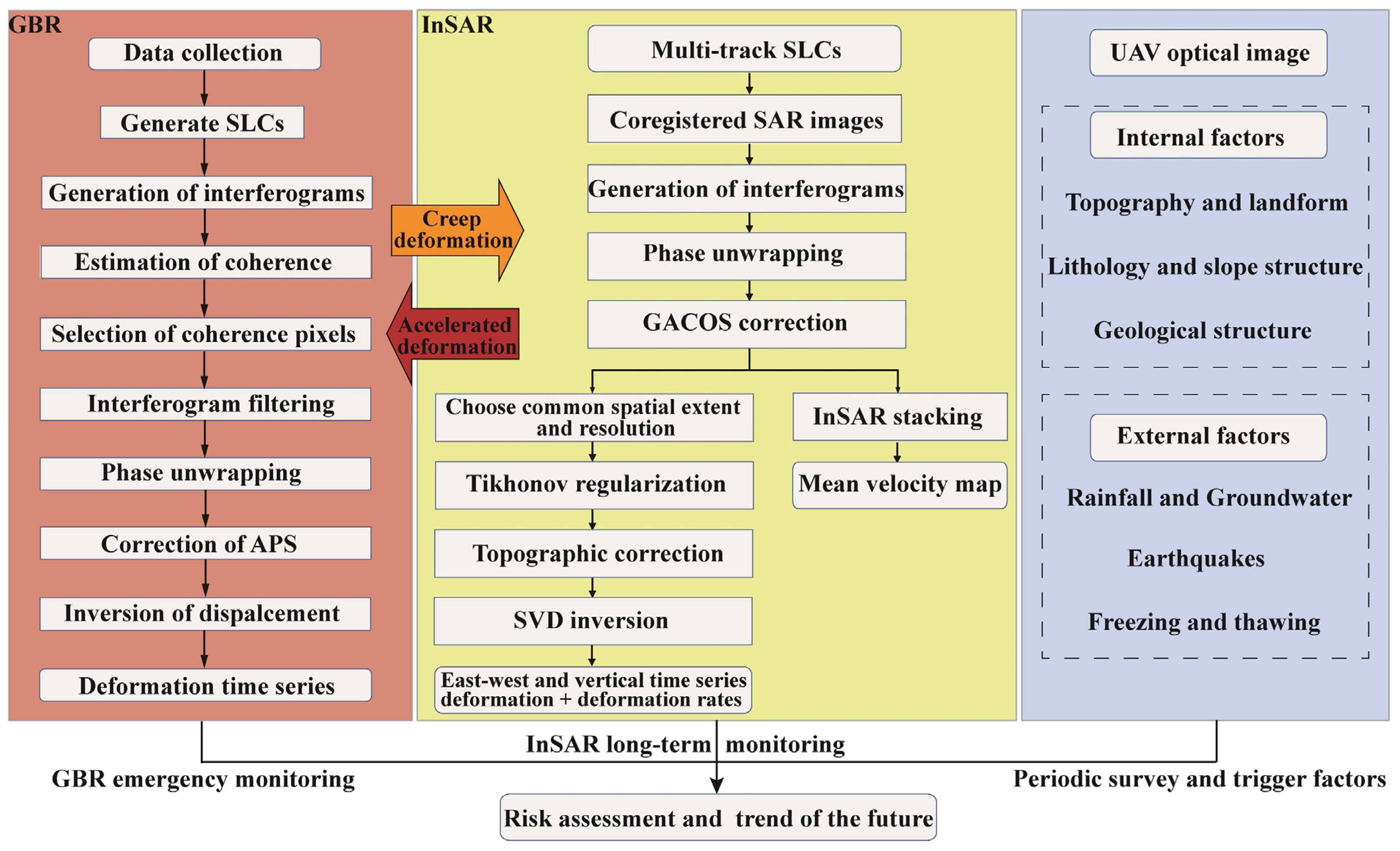
2. Materials and Methods

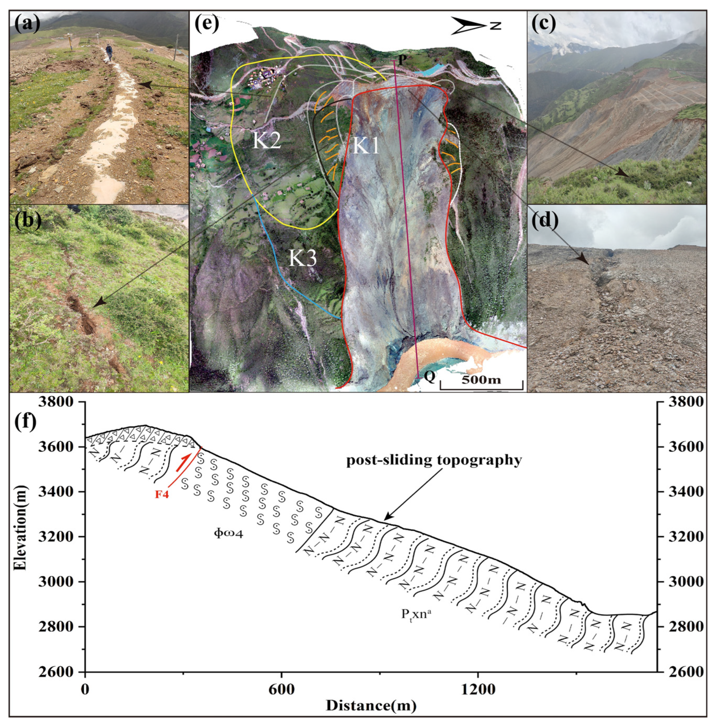
2.1. Study Area

The Baige landslide area is situated in the northern Hengduan Mountains of the eastern Qinghai-Tibet Plateau, within the Jinsha River valley region between the Mangkang Mountain and the Shaluli Mountain. The landform type is an alpine canyon landform resulting from tectonic erosion, and river erosion is significant. The landslide lies in the ‘V-shaped’ Jinsha River valley, with the Jinsha River concave bank on the front edge and the bank shoulder on the back, as indicated in Figure 1c. The topography of the landslide is steep, with the front edge of the landslide sloping at around 65°, the center and rear sections sloping at 35~55°, and the back of the landslide sloping at 75°. The elevation of the rear edge of the landslide is about 3720 m, the elevation of the toe is about 2880 m, and the drop is 840 m. The collapse caused a surge of up to 160 m on the left bank. A barrier dam is formed when shovels on the left bank collide, assemble, bounce, and disperse to the right bank [6]. The landslide is located in the Jinsha River suture zone (Figure 1b), near the Jiangda–Boluo–Jinshajiang fault zone and NW-trending fault, with the regional Boluo–Muxie reverse fault at the rear of the landslide. The landslide border has distinct features, and the lithology of the landslide body is primarily gneiss. The range along the landslip bed from the back border to the center is green-gray serpentine, with an elevation of 3400~3700 m, while the middle and front part below the elevation of 3400 m is the Proterozoic Xiongsong Group gneiss formation, including biotite plagioclase gneiss, hornblende plagioclase gneiss, plagioclase amphibolite, and greenschist. The landslide exhibits multistage deformation and metamorphism, and the mylonite and alteration are quite severe [26]. The climate in this area is chilly and the vertical characteristics are obvious due to the semi-humid climate in the plateau cool temperate zone.

2.2. Ground-Based Radar Interferometry

From 4 December to 10 December 2018, a GBR interferometry system (GPRI-II) was used to monitor the Baige landslide. The incidence angle of the antenna was adjusted at 5° below the horizontal, which maximized the equipment’s sensitivity to displacement. The deployment position was at a distance of about 8 km opposite to the landslide, the rotation angle of equipment was 35°, and the effective observation distance was 6.5~9 km, with a range resolution of 0.75 m and an azimuth resolution of 6.8 m/km. The time resolution was 10 min, and 778 images were collected.

Table 1. Key parameters of GBR observations.

Parameters	Values
Acquisition dates	4 December 2018–10 December 2018
Radar frequency (GHz)	17.2
Effective measurement range (km)	6.5~9
Revisiting times (min)	10
Incidence angle (°)	−5
Center azimuth angle (°)	270

lists the imaging parameters of GBR in detail.

This paper employs the notion of a small baseline subset (SBAS) and processes continuous GBR images on the basis of a unit. The processing flow mainly includes data preprocessing, interferogram generation, coherence estimation, coherent point extraction, interferogram nonlocal filtering, phase unwrapping (3D), atmospheric correction, displacement inversion, time-series analysis, and geocoding [27]. The GBR interferometry and spaceborne InSAR time-series analysis procedures are comparable. The greatest distinction is that GBR has a zero spatial baseline and does not need image registration or terrain phase compensation.

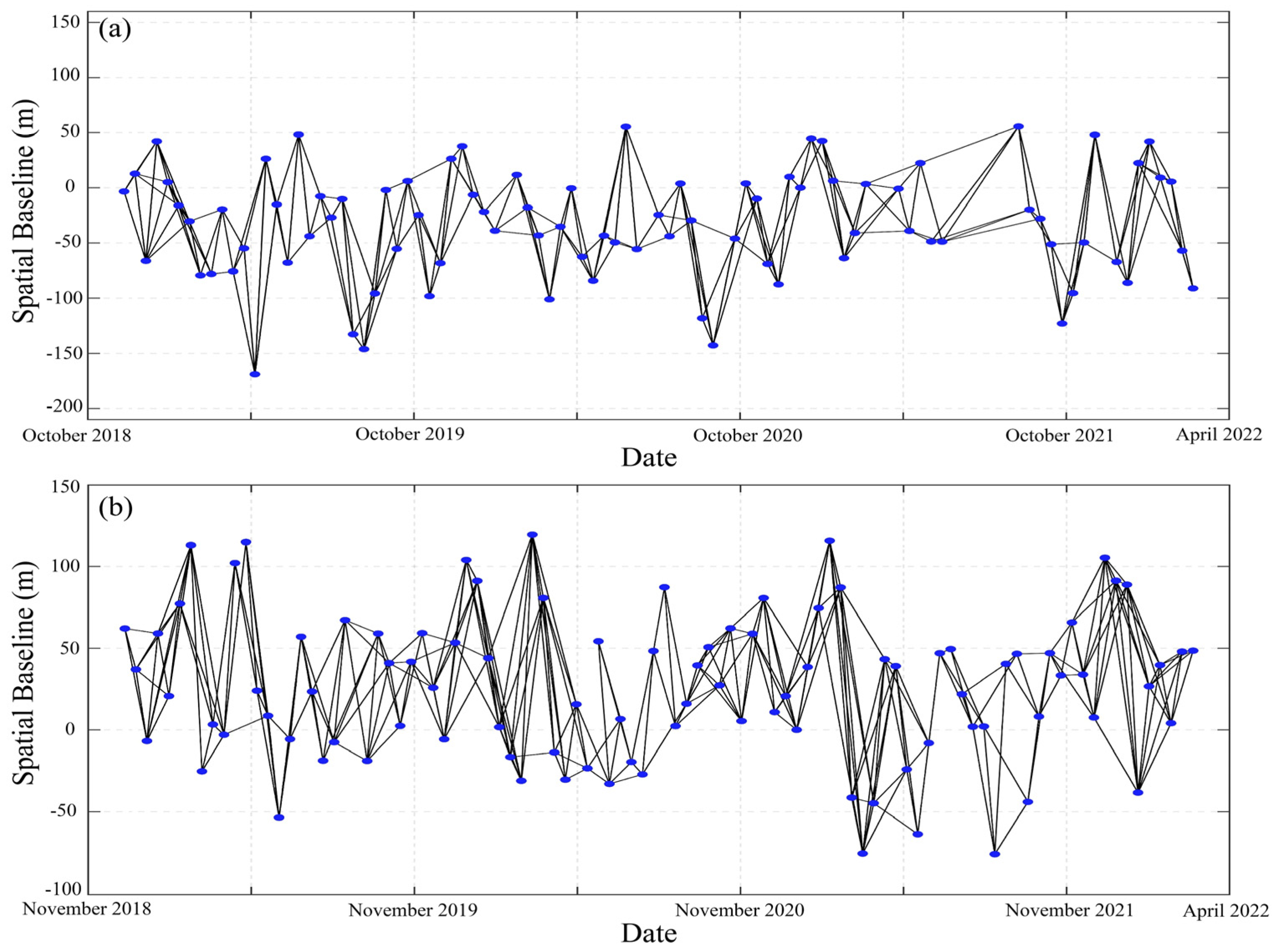
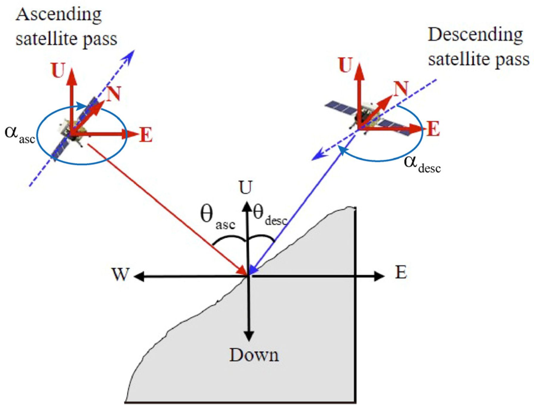
2.3. Spaceborne Radar Interferometry

Due to the influence of SAR image geometric distortions (i.e., layover, foreshortening, and shadow) and the limitation of the LOS surface deformation, the differences between the InSAR results of a single platform or orbit and the actual deformation of the landslide body can be too great to satisfy the engineering requirements of landslide monitoring [28]. Therefore, we obtained two Sentinel-1A datasets covering the Baige area from December 2018 to February 2022.

Table 2. Sentinel-1A image data information.

Path	99	33
Orbit	Ascending	Descending
Incidence angle (°)	36.3	44.2
Heading angle (°)	−12.78	192.78
Number of images	87	97
Acquisition period	14 December 2018–20 February 2022	21 December 2018–27 February 2022

lists the Sentinel-1A image data information, and their coverages are shown as the rectangles in Figure 1a.

We selected high-quality interferograms and set a time baseline threshold of 36 d and a spatial perpendicular baseline threshold of 200 m (Figure 2). A common strategy to minimize coherence loss is to use interferograms with short time baselines. However, it has recently been shown that using this strategy can introduce a bias [29,30,31]. Although the bias caused by such inconsistencies is small in each individual interferogram, its accumulation in time could impact the final estimated velocities [32]. Note that the deformation rate of the landslide is 2–3 orders of magnitude larger than the impact, and hence the bias was neglected in this study. The Shuttle Radar Topography Mission (SRTM) DEM [33] data with a 30 m spatial resolution released by NASA were used to eliminate the terrain phase and geocode.

2.3.1. GACOS-Assisted InSAR Stacking

The electromagnetic wave signal emitted by SAR satellite radar has a tropospheric delay when passing through the Earth’s atmosphere, which could result in an error of about 20 cm in the interferograms [34]. It is difficult to separate the actual deformation signal from the tropospheric delay, especially the small long-wavelength deformation signals [12]. Due to the spatially stratified effects of water vapor and temperature, the tropospheric delay shows a significant correlation with the surface fluctuation on the interferogram, especially in mountainous areas [35]. To correct the atmosphere of the interferograms, we applied the generic atmospheric correction online service (GACOS) products to each interferogram. GACOS utilizes the European Centre for Medium-Range Weather Forecasts (ECMWF) high-resolution (HRES) atmospheric model and the iterative tropospheric decomposition (ITD) model to separate stratified and turbulent signals from the total tropospheric delay [36]. It provides users with free, near-real-time, and global coverage of InSAR atmospheric delay error correction mapping, which can be used to correct the atmospheric delay error of InSAR measurement [37,38], and has been successfully applied to plateau mountainous areas by numerous researchers [34,39,40]. The basic assumption of InSAR-stacking technology is that the surface deformation is linear and there is no nonlinear change. Its advantages include a high operation efficiency, which can effectively weaken the influence of random errors. The zenith total delay (ZTD) product introduced by GACOS diminishes the atmospheric error [38], and the residual atmospheric error can be considered as a random error; thus, the signal-to-noise ratio can be improved by InSAR-stacking technology. The unwrapped phase following GACOS correction is averaged using the least square method, and the interferometric phase is weighted by the time interval [41]. The LOS annual deformation rate is obtained [34,42].

$$V_{mean}=\frac{\lambda }{4\pi }\frac{{\displaystyle {\sum }_{i=1}^N{\phi }_i\mathsf{\Delta }{T}_i}}{{\displaystyle {\sum }_{i=1}^N\mathsf{\Delta }{T}_i{}^2}}$$

(1)

where $\lambda$ is the radar wavelength, $V_{mean}$ indicates the mean velocity, ${\phi }_i$ indicates the unwrapped phase after GACOS correction, and $\mathsf{\Delta }{T}_i$ indicates the time span of the interferogram.

2.3.2. MSBAS InSAR

InSAR observations from a single orbit can only be used to acquire the Earth’s surface deformation along the satellite LOS direction since the SAR imaging geometry is side-looking. The generation of multidimensional deformation and the deformation time series is beneficial because landslides can move in different directions for different sections. Note that the sliding direction of the Baige landslide is in the east–west direction, and InSAR measurements are insensitive in the north-south direction because of the near-polar flighting of satellite radar; thus, the north–south component of the Earth’s surface deformation was neglected in this study. The MSBAS method is a multidimensional deformation time-series analysis method [43,44], which is derived from the SBAS InSAR [45]. The image covering the common area is selected based on the different incident angles and azimuth angles from ascending and descending orbits. The LOS direction deformation is decomposed according to its geometric relationship (Figure 3), which not only enhances the temporal density of surface observation but also obtains the two-dimensional deformation field (east–west and vertical directions) of the pixels [46].

When only one set of SAR data is acquired, the traditional SBAS method is able to invert the LOS displacement time series [45].

$$\{\begin{array}{l}A{V}_{\mathrm{los}}={\varphi }_{\mathrm{obs}}\\ d_{\mathrm{los}}^{i+1}=d_{\mathrm{los}}^i+V_{\mathrm{los}}^{i+1}\mathsf{\Delta }{t}^{i+1}\end{array}$$

(2)

where $A$ is a design matrix constructed from the time intervals of the interferometric pairs, $V_{\mathrm{los}}$ represents the LOS mean velocity, ${\varphi }_{\mathrm{obs}}$ represents the interferometric phase, and $d_{\mathrm{los}}^i$ is the LOS displacement at epoch $t^i$. Once $K$ independent SAR datasets with different orbital geometries (azimuth $\alpha$ and incidence angle $\theta$) are acquired, $V_{\mathrm{los}}$ can be expressed by the velocity in the north, east, and up:

$$V_{\mathrm{los}}=SV=S_{\mathrm{N}}{V}_{\mathrm{N}}+S_{\mathrm{E}}{V}_{\mathrm{E}}+S_{\mathrm{U}}{V}_{\mathrm{U}}$$

(3)

where $V$ is a velocity (ground deformation rate) vector with the components of $V_{\mathrm{N}},V_{\mathrm{E}},V_{\mathrm{U}}$; $S$ is a unit vector with the projection components of $S_{\mathrm{N}},S_{\mathrm{E}},S_{\mathrm{U}}$:

$$S=[S_{\mathrm{N}}\begin{array}{c}\end{array}{S}_{\mathrm{E}}\begin{array}{c}\end{array}{S}_{\mathrm{U}}]=[\sin \theta \sin \varphi \begin{array}{c}\end{array}-\cos \theta \sin \varphi \begin{array}{c}\end{array}\cos \varphi ]$$

(4)

Equation (2) can be rewritten for each SAR dataset $k=1,2,\mathrm{\dots },K$:

$$[A{S}_{\mathrm{N}}^k\begin{array}{c}\end{array}A{S}_{\mathrm{E}}^k\begin{array}{c}\end{array}A{S}_{\mathrm{U}}^k]\cdot {[V_{\mathrm{N}}\begin{array}{c}\end{array}{V}_{\mathrm{E}}\begin{array}{c}\end{array}{V}_{\mathrm{U}}]}^T={\varphi }_{\mathrm{obs}}^k$$

(5)

When $K$ independent SAR datasets are involved and the $k^{\mathrm{th}}$ dataset consists of $M^k$ interferometric phase measurements generated from $N^k$ SAR images (i.e., $N^k$ epochs), the MSBAS method can be explained by the following form [43]:

$$\left[\begin{array}{c}{A}^1\\ A^2\\ \stackrel{\dots }{A^K}\end{array}\right]\left[\begin{array}{c}{V}^1\\ V^2\\ \stackrel{\dots }{V^{{\sum }_{k=1}^K{N}^k-1}}\end{array}\right]=\left[\begin{array}{c}{\varphi }^1\\ {\varphi }^2\\ \stackrel{\dots }{{\varphi }^K}\end{array}\right]\begin{array}{cc}\begin{array}{cc}& or\end{array}& \widehat{A}\widehat{V}=\widehat{\varphi }\end{array}$$

(6)

where the new matrix $\widehat{A}=[A{S}_{\mathrm{N}}^{}\begin{array}{c}\end{array}A{S}_{\mathrm{E}}^{}\begin{array}{c}\end{array}A{S}_{\mathrm{U}}^{}]$ with the dimensions of ${\sum }_{k=1}^K{M}^k\times 3({\sum }_{k=1}^K{N}^k-1)$, the new vector $\widehat{V}$ has the dimension of $3({\sum }_{k=1}^K{N}^k-1)\times 1$, and the new vector $\widehat{\varphi }$ has the dimension of ${\sum }_{k=1}^K{M}^k\times 1$. Due to the near polar orbits of Sentinel-1, LOS measurements are least sensitive to displacements in the north–south direction. Equation (6) can be simplified by [43]:

$$\left[\begin{array}{c}\widehat{A}\\ \xi L\end{array}\right]\left[\begin{array}{c}{V}_{\mathrm{E}}\\ V_{\mathrm{U}}\end{array}\right]=\left[\begin{array}{c}\widehat{\varphi }\\ 0\end{array}\right]$$

(7)

where $\xi$ is the regularization parameter and $L$ is an identity matrix.

Figure 4 shows the landslide-monitoring framework used in this study to combine GBR and spaceborne InSAR observations with unmanned aerial vehicle (UAV) optical images to provide technical support for landslide long-term and emergency monitoring and landslide development trend analysis. Long-term and emergency technologies are adjusted by the rate of deformation. Spaceborne SAR is used in the creep stage, and GBR is used when accelerated deformation rates are detected. At the same time, combined with UAV optical images, internal geological conditions, and external trigger factors, the risk assessment and future development trend analysis of the landslide are carried out.

3. Results

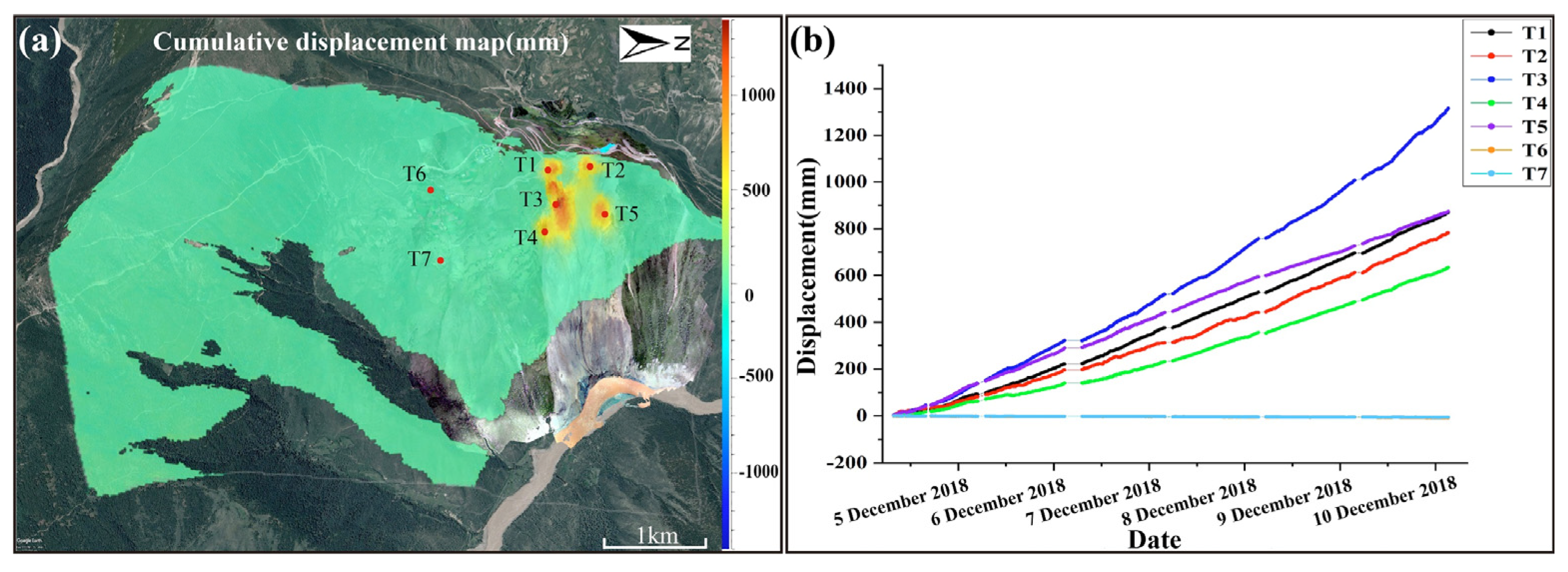
3.1. Ground-Based Radar Results

The aforementioned methods were used in this study to process GBR data and generate the accumulated deformation of the Baige landslide in the LOS direction (Figure 5a). Red (positive value) represents the movement towards the radar instrument. As shown in Figure 5, from 4 to 10 December 2018, the deformation area is primarily concentrated near the rear edge of the landslide, with a maximum cumulative displacement of 1.4 m.

The feature points of the primary deformation areas are subjected to time-series analysis. Figure 5a depicts the location of the feature points, where T1–T5 are on the landslide body and T6 and T7 are far away from the landslide. Points T1–T5 quickly moved to the radar system during the observation period and all of them had the same movement trend, indicating that active sliding occurred. Note that the displacement of Point T3 was the largest. Points T6 and T7 basically remained in a stable state (Figure 5b). The post-event deformation changed rapidly, reaching hundreds of millimeters per day or even larger, which was much larger than the deformation gradient that can be monitored with spaceborne InSAR technology. Therefore, it is necessary to use GBR for emergency monitoring.

According to the GBR monitoring results of the Baige landslide over 6 days, there were still obvious surface displacements. Thus, periodic field surveys and Sentinel-1A data were employed for continuous monitoring to increase the attention to the changing trend of the landslide.

3.2. Spaceborne InSAR Results

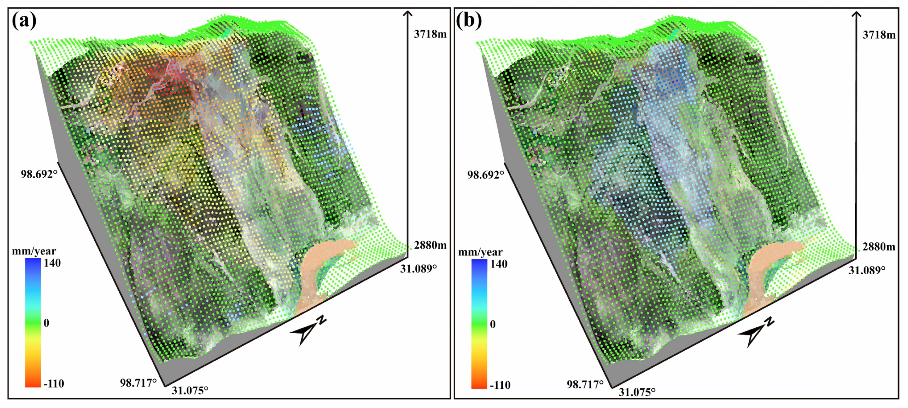
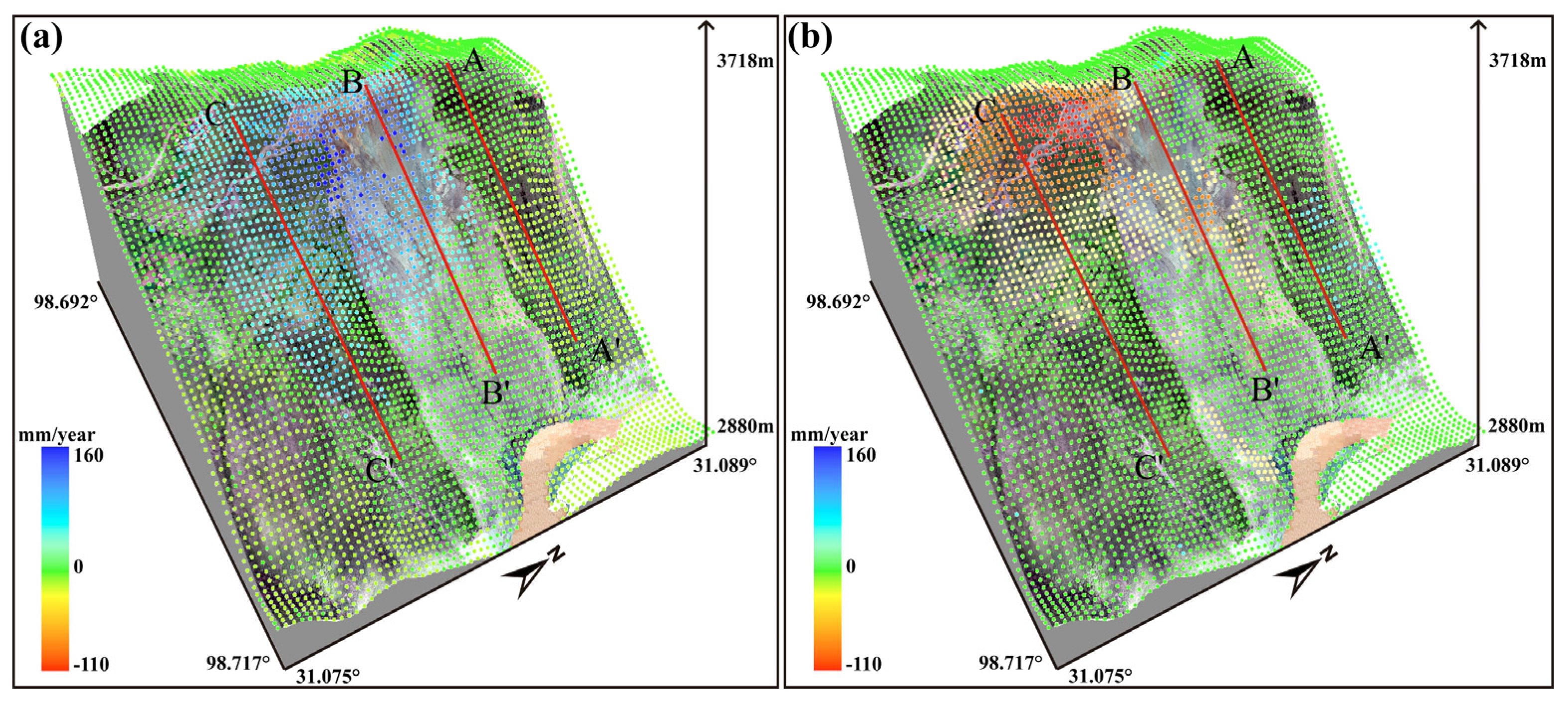
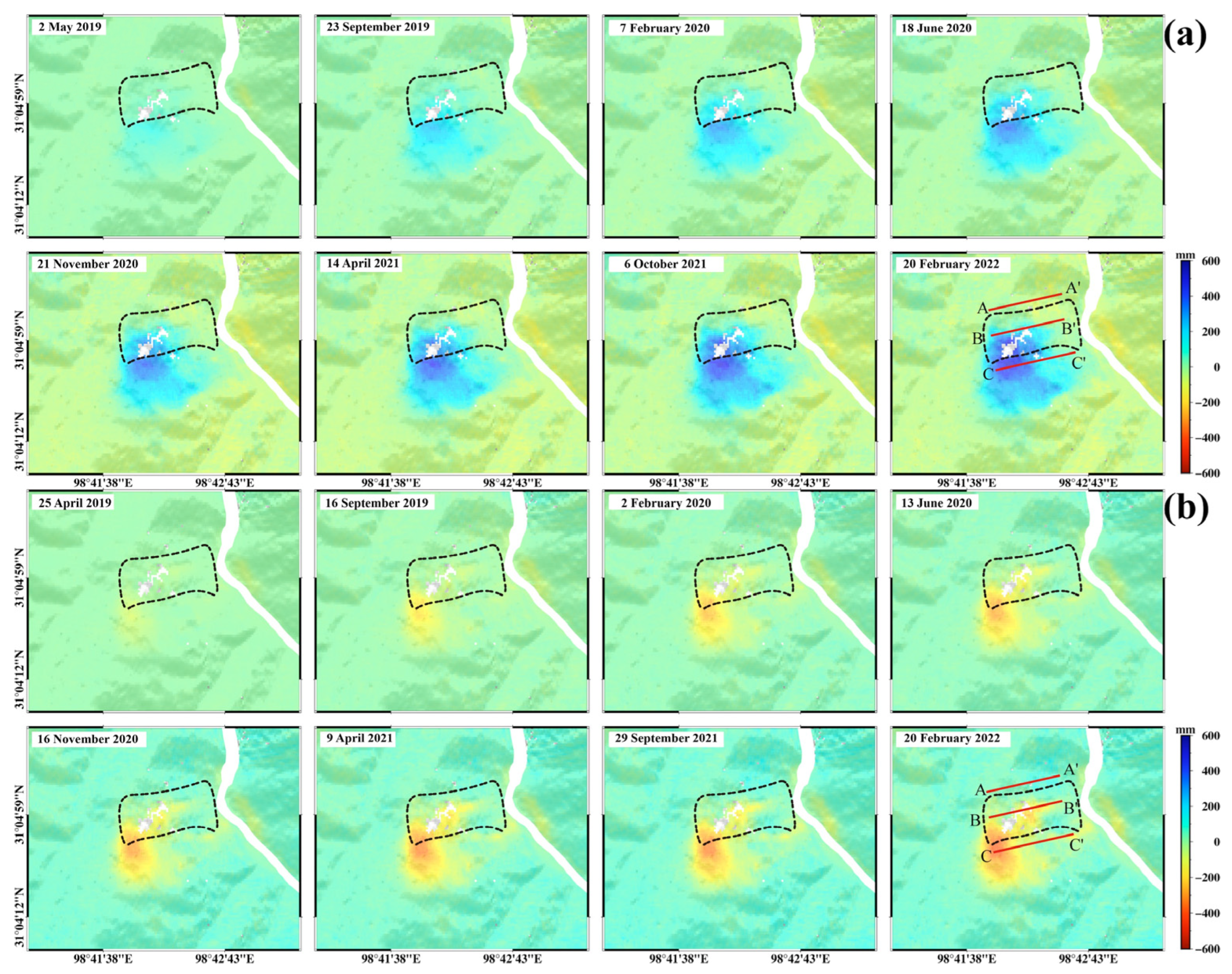
3.2.1. LOS Direction Deformation

Figure 6 shows the LOS annual surface deformation rate of the landslide generated by GACOS-assisted InSAR stacking. The topographic relief was constructed utilizing UAV optical images and SRTM DEM. The distribution and magnitude of the deformation fields from ascending and descending orbits are clearly different. The maximum annual LOS deformation rate of the ascending orbit is 110 mm/year, whilst that of the descending orbit is 140 mm/year. The spatial features of the Baige landslide revealed by InSAR stacking indicate that it has experienced remarkable deformation. The deformation extended outward from the mountain top, and with the increase in range, the deformation scale gradually decreased until it covered the whole Baige village. Furthermore, the deformation only in the LOS direction is insufficient to estimate the real kinematic process of the landslide. Despite the fact that the stacking findings based on single-orbit SAR images can successfully identify the range of active landslides, the observed results cannot properly depict the actual deformation of landslides owing to the impact of the LOS on the observation viewpoint of landslide deformation.

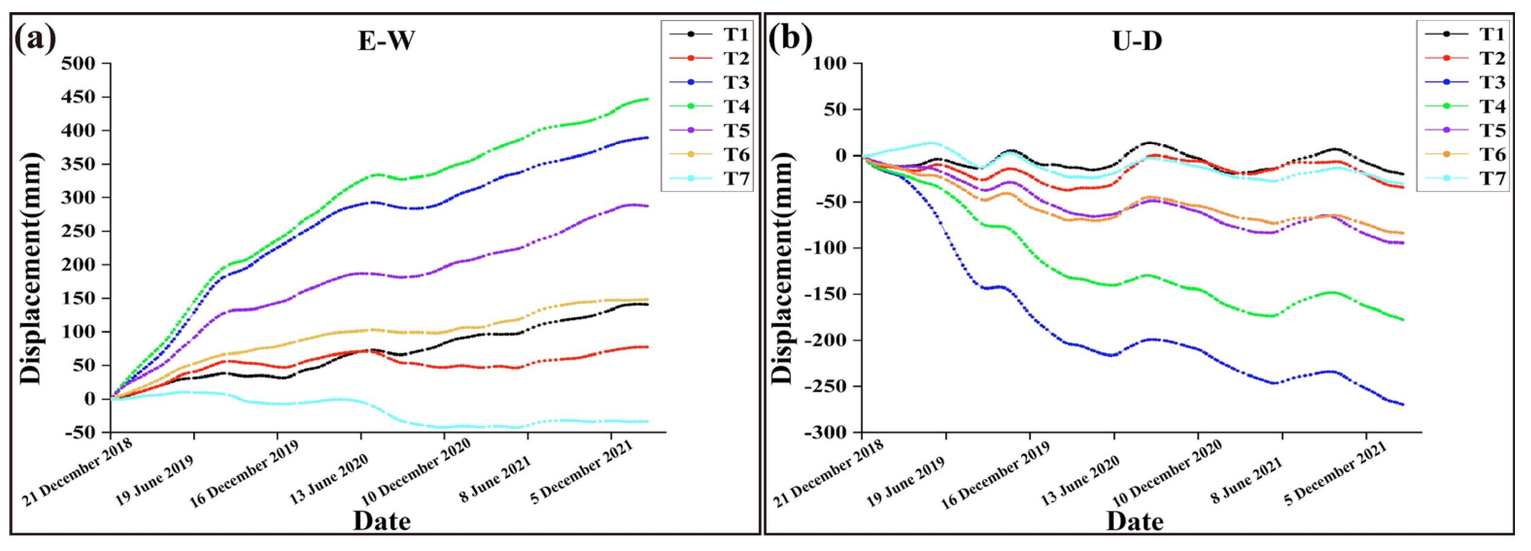
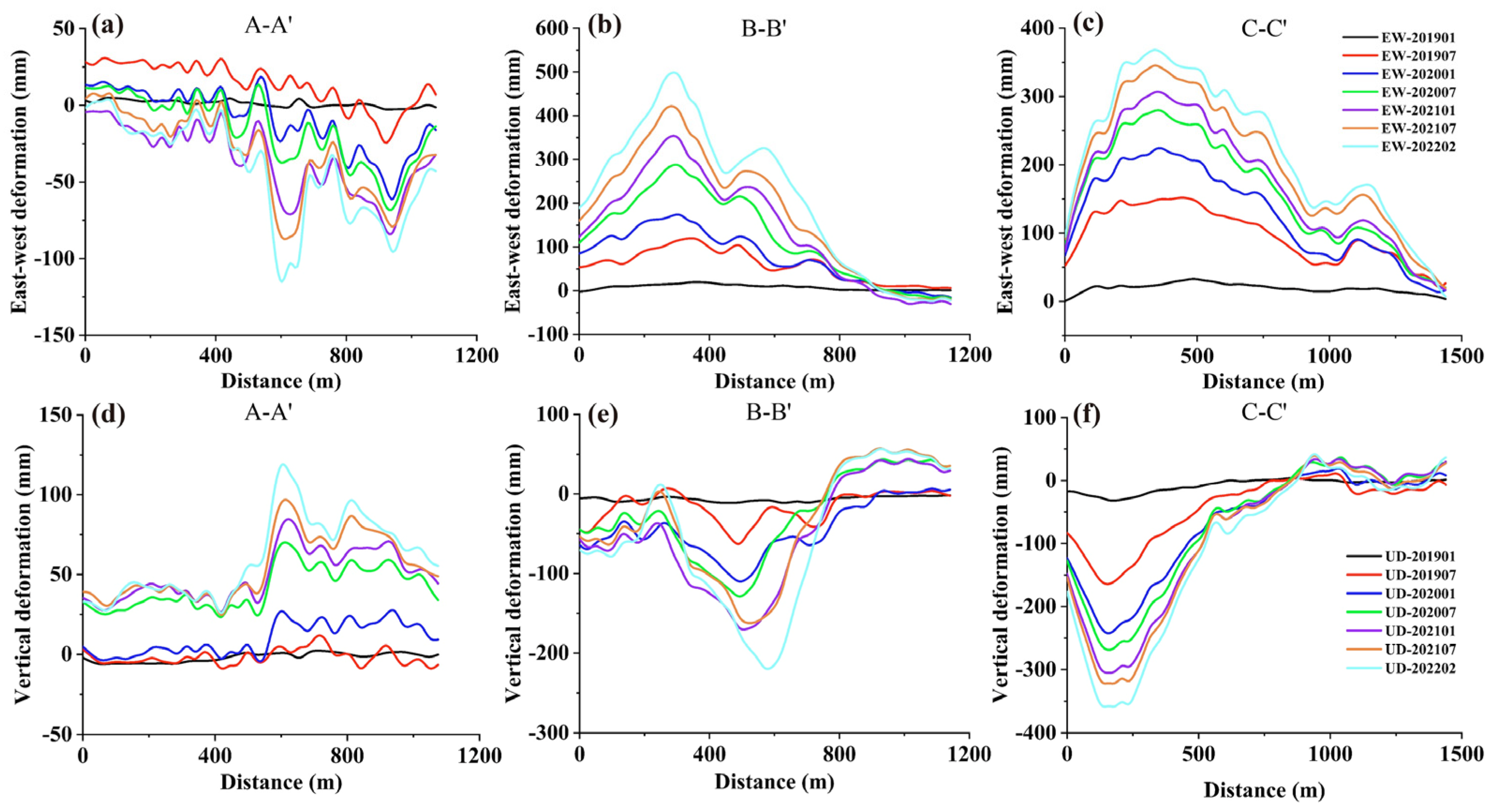
3.2.2. Two-Dimensional Deformation

Since the Baige landslide is an east–west landslide, it can be effectively analyzed by decomposing the deformation into the vertical and east–west components. Consequently, the MSBAS method was employed to explore the movement process of the Baige landslide.

In Figure 7a, the positive values indicate eastward displacements and negative values represent westward displacements. In Figure 7b, the positive values represent uplift and the negative values represent subsidence. From the two-dimensional deformation rate maps, the maximum annual deformation rates in the east–west and vertical directions are 170 mm/year and 100 mm/year, respectively. The deformation is concentrated at the rear edge and in the middle and rear parts of the landslide. The deformation in both directions overlaps in a large proportion, indicating that the slope moves east along with the settlement. The phenomenon of incoherence can be observed in parts of the landslide, which were likely caused by the large gradients of landslide deformation.

Figure 8a shows that during the period from December 2018 to February 2022, in the east–west direction, the deformation area expanded from the initial landslide body to the right side of the landslide. In the vertical direction, the deformation area expanded to the right and rear.

To track the subsequent movement state of the landslide deformation area monitored by GBR, the same feature points T1–T7 were selected in the two-dimensional deformation. Figure 9 shows the time-series results. Since spaceborne InSAR observations span different time intervals from GBR observations, they are not comparable in terms of magnitude but the development trends of feature points could be interesting. Points T1 and T2 are located at the rear edge of the landslide, their cumulative displacements from GBR observations were close to 800 mm, but their cumulative displacements in the east–west and vertical directions from spaceborne InSAR were less than 100 mm. Points T3, T4, and T5 exhibited large displacements in the east–west and vertical directions, showing similar movement trends to the GBR results. Points T6 and T7 are far away from the landslide, and no obvious displacement can be observed with GBR. However, spaceborne InSAR observations reveal that the deformation of Point T6 was 140 mm in the east–west direction and nearly 100 mm in the vertical direction during the long-term monitoring period. The cumulative displacement at Point T7 was much smaller, within 50 mm in both directions.

As shown in Figure 10, the landslide changed significantly from December 2018 to December 2019. In 2020–2022, the cumulative deformation gradually increased, but the acceleration trend obviously decreased, which may be due to the large residual sliding trend in the following year after the second Baige landslide, and then the deformation rate gradually decreased.

4. Discussion

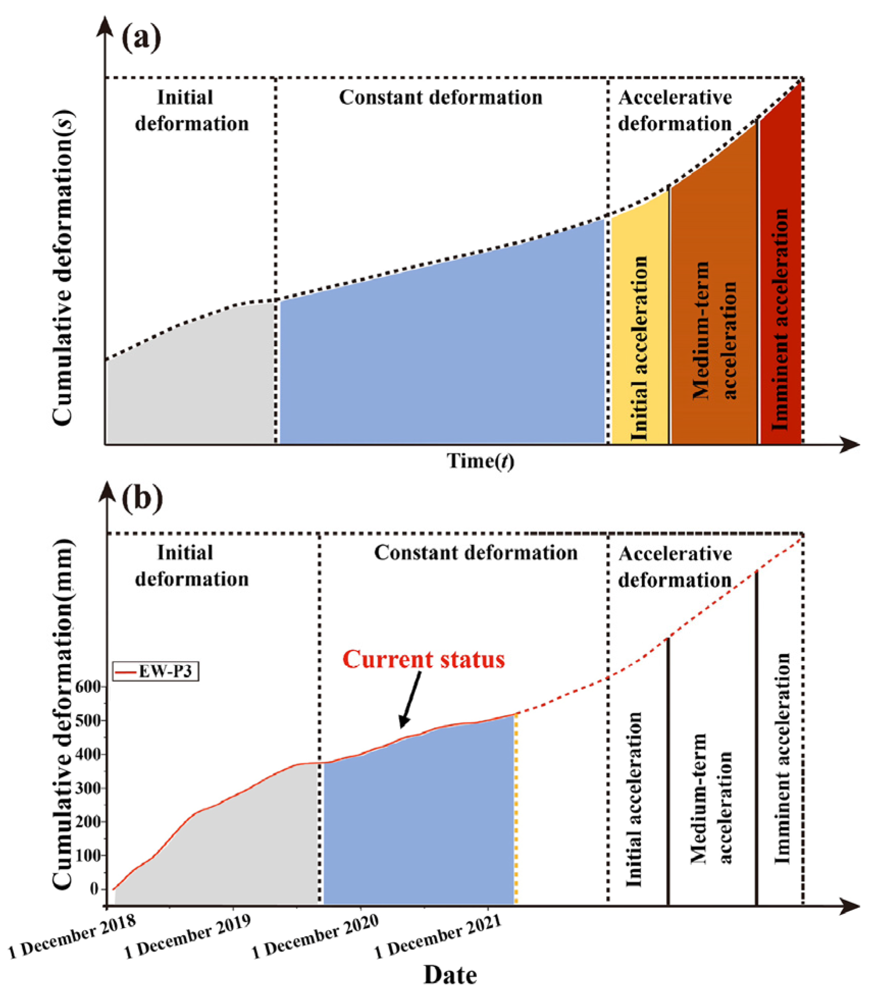
4.1. Analysis on Development Trend of the Baige Landslide

4.1.1. Long-Term Monitoring Results and Deformation Stages

To further comprehend the deformation trend of the landslide, six feature points (Figure 11a) are selected on the landslide body and their point time series are analyzed in conjunction with the deformation rate map and characteristics of optical images. Figure 11b demonstrates that the MSBAS method considerably densifies the deformation time series, with the lowest time period being just 2 days. The red curve depicts the east–west deformation, while the black curve depicts the vertical deformation.

Point P1 is close to the left side of the landslide’s rear edge. According to the deformation time series of Point P1, it is essentially stable. Point P2 is in the middle of the landslide, moving in the east–west direction at a constant speed, while the vertical direction was essentially stable before 2021 and in a state of acceleration from 2021 to 2022. Point P3 is on the right side of the rear edge of the landslide, and its accumulated displacement is 520 mm in the east–west direction and is close to 260 mm in the vertical direction. The displacement rate of Point P3 before June 2020 was obviously greater than that after June, and Point P3 was in a constant motion state in both directions after June 2020. P4 is at the right rear of the landslide trailing edge, with a large cumulative deformation in both directions, close to 400 mm, and the rate after June 2020 was clearly lower than before. Points P5 and P6 are on the right side of the landslide, and both were in a stage of slow deformation. In conjunction with the monitoring data of GBR, it is evident that the deformation area extended to the right of the landslide’s trailing edge. Based on the association between the overall change trend of the characteristic points and the daily precipitation value, only Point P2 exhibited accelerated sliding when it lagged behind the rainy season for 1~3 months, whilst the other characteristic points had no obvious relationship with precipitation. Therefore, the changes in the landslide cannot be attributed to rainfall alone.

One common requirement for landslide failures is that the slope deformation has reached the rapid deformation stage. The time series of P3 from the east–west direction in Figure 11b is chosen, and the change characteristics are compared using the “three-stage” theory [47] of deformation and landslide failure. Figure 12a illustrates the standard creep curve of a landslide. The deformation and time curve is in a constant state of change, particularly when the deformation reaches the accelerated deformation stage. The curve tends to continually increase. During the stage of near-sliding, the deformation curve is almost vertical. It can be used for early warning and forecast analysis by the features of the deformation–time curve in the process of slope development. The Baige landslide is now progressing at a consistent rate (Figure 12b), and its evolution in the future needs ongoing monitoring.

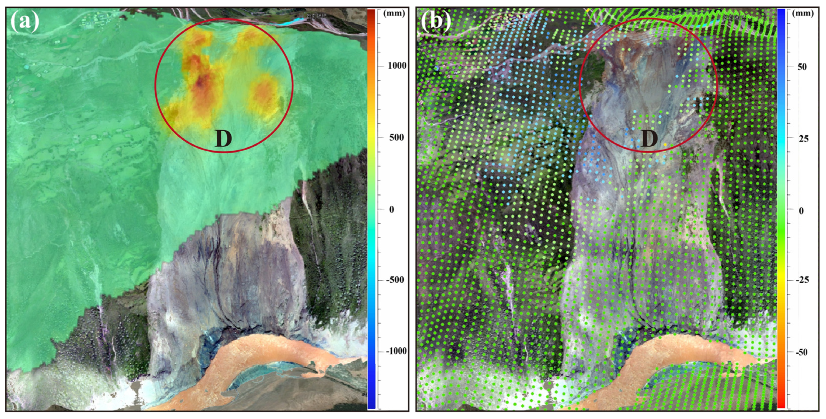
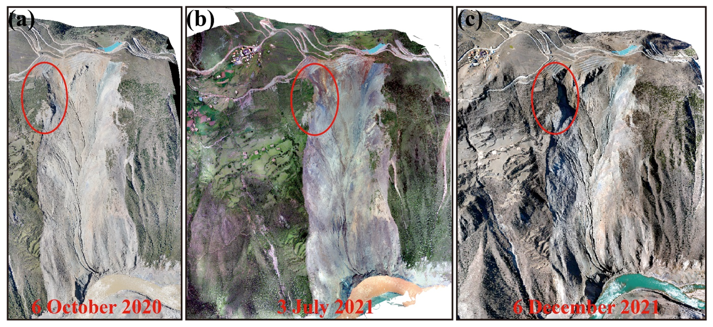
4.1.2. Comprehensive Analysis Based on UAV Optical Images, Periodic Field Surveys, GBR, and InSAR Results

In the acceleration stage, due to the rapid deformation rate of landslides, spaceborne InSAR may not be able to monitor the deformation. In this study, GBR observations span the period from 4 December to 10 December 2018, which was very close to the last landslide. The deformation rate monitored by GBR was 220 mm/d, far exceeding the detectable gradient of spaceborne InSAR. As can be seen from Figure 13, the InSAR results are partially incoherent, and the displacements for certain coherent points in Area D are greatly underestimated. Therefore, it is proposed to combine the long-term spaceborne InSAR monitoring in the creep period with the emergency monitoring in GBR in the acceleration period to establish a framework that can monitor the whole landslide period to ensure the integrity of landslide monitoring. Due to the low overlap between the monitoring time of GBR and the time of spaceborne SAR, the combination of the two technologies at the data level is not enough, which is an inherent defect of the data. Among them, the advantages of GBR are its high resolution (high spatial resolution, short sampling period), near-real-time monitoring, being unaffected by weather, high sensitivity (small changes can be detected), and high accuracy (theoretically, sub-millimeter target deformation detection accuracy can be achieved). However, its shortcomings are obvious, including the deformation information of the target in the line of sight of the radar (three-dimensional deformation in a geodetic coordinate system can be obtained with the assistance of other measuring means), limited detection range (comprehensive information may not be obtained in certain remote areas or areas with many obstructions), and high cost (the instrument of GBR is expensive, and the training and maintenance of technicians also need some investment, which makes the use cost higher). Therefore, if the two technologies can be reasonably combined, it can not only save manpower and material resources but also better explain the landslide deformation and provide a more powerful guarantee for landslide monitoring.

In the creep stage, the landslide deformation trend is exhaustively evaluated using optical visual interpretation (Figure 14), periodic field research (Figure 15), and spaceborne InSAR monitoring results. The main deformation region is situated on the right side of the landslide’s downstream border, which is primarily generated by the sliding and traction of two landslides. According to the varying degrees of distortion, it can be roughly divided into three deformation areas, namely K1, K2, and K3 (Figure 15e).

The majority of the deformation area is to the right of the landslide border. Affected by the traction of two landslides, the deformation in the area consists mainly of transverse tensile cracks, longitudinal tensile cracks, and dislocation deformation. After the Baige landslide occurred, the free face surface increased, and the unstable mass in the K1 area moved to the lower right side. On the slope surface in this area, numerous transverse and longitudinal tension fractures developed. The rear edge tensile cracks penetrated, and the right side developed through shear cracks. Its material mainly consisted of quaternary eluvial block gravel soil, as well as gneiss and phyllite of the Xiongsong Group in the Proterozoic (Figure 15f).

The deformation in the K2 and K3 areas is relatively small. Area K2 is located at the upper right of Area K1. Affected by the deformation and traction of Area K1, the signs of deformation in this area include a tensile crack at the rear edge, a discontinuous tensile crack at the middle, and a tensile crack at the rear edge. The traction of two slides forms the K2 and K3 areas, and the leading edge is bounded by the scarp caused by the K3 slip. The back edge is bounded by the K2 subsidence range, which is an irregular strip shape in plan. The material is mainly composed of quaternary residual slope block gravel soil, as well as Proterozoic Xiongsong Group gneiss and phyllite. The fractures in the K1 area are densely developed, primarily in the rear back edge and center of the slope, with penetrating fractures in the rear edge. The K1 area below the surface within 7 m is mainly quaternary debris and loose material, below 7 m is lithology exposure, and the integrity of the exposed rock mass is in excellent condition. Thin residual slope deposits cover the surface of the K2 and K3 areas, exposing the lithology underneath. The predominant exposed lithologies are gneiss and schist. Among them, 2~15 m is fully weathered gneiss. The integrity of the rock mass is poor and the structure is shattered. The rock mass of 15~45 m is strongly weathered schist, 45~75 m is strongly weathered gneiss, and the rock mass results are relatively favorable [48]. Therefore, it is more probable that the shallow portion of the K1 area would collapse and deform due to the dense development of cracks in the region and the presence of a specific thickness of covering layer on the slope surface. In the middle and rear areas of K2 and K3, the rock mass structure is fractured within 15 m below the surface, and there is a possibility of instability. Since the terrain in the middle and rear areas is relatively flat, the cracks in the area have not developed. Furthermore, they are blocked by K1, reducing the likelihood of instability. Note that if K1 becomes unstable, the shattered rock mass in K2 and K3 will be influenced by its traction, and sliding and instability are also possible.

According to the current motion state and geological conditions, the Baige landslide may have two development trends: (i) The self-adjustment state of the residual movement after the occurrence of large landslides will develop in a stable direction; (ii) The landslide is in the development state of energy accumulation again, and the potential sliding surfaces and failure mechanisms in the deformation area mainly involve the shallow sliding of residual slope deposits on the surface. The deformation in K1 is relatively strong, the front and middle parts of the deformation area face empty spaces with steep faces, and the rock mass structure is broken. Affected by the Baige landslide traction, the rock mass is further loosened and readily slides downwards, with a “creep-tensile fracture” being the predominant form of failure. In addition, it should be noted that under the infiltration of rainy season precipitation, the deformation in the front of the deformation area will be intensified, making the through cracks widen and deepen continuously, and the abrupt terrain change in front of the deformation zone is likely to cause overall instability, which increases the risk of river blocking.

4.2. Driving Factors of the Surface Motion of the Baige Landslide

Typically, landslides are determined by internal geological conditions and external triggering factors, including slope structure, lithology, slope topography, and external driving factors such as earthquakes, rainfall, groundwater, and human activities [49].

4.2.1. Internal Geological Conditions

The location of the Baige landslide is a V-shaped canyon terrain, with steep terrain and a significant change in altitude. From the top of the landslide to its foot, the overall trend is steep–slow–steep. The slope of the landslide changes significantly (Section 2). The slope has an elevation difference between the toe and top of about 850 m, and the favorable topography makes long-term gravity creep a common feature of catastrophic landslides [50].

The rear and deep parts of the slope are mainly green-gray serpentine, which is generally fragmented. The middle part is mostly gray-dark gray and locally gray-black banded gneiss. The two strata are unconformity contact surfaces, and the rock mass is highly fractured. It has more fragmented, sand-like features and is more sensitive to water (such as rainwater infiltration and groundwater), making it more susceptible to disintegration. The creation, expansion, and merging of cracks and craters will ultimately degrade the rock mass quality. The comparatively firm upper and soft lower shattered rock mass structure will provide better material conditions for landslide initiation [48].

The Baige landslide is situated in the suture zone of the Jinsha River, near the Jiangda–Boluo–Jinshajiang fault and NW-trending fault zone, and the regional Boluo–Muxie reverse fault is positioned at the dorsum of the landslide (Figure 1b). Long-term fault zone actions will degrade the integrity and quality of the rock masses on both sides, weaken the anti-erosion ability, and lower the stability. The steep rock mass at the back of the landslide and the interaction of serpentine with gneiss create an incredibly unfavorable environment for landslide development.

4.2.2. External Triggering Factors

As the trigger mechanism for rainy landslides [51], rainfall will soften and muddy the rock mass along the landslide cracks, reducing its shear strength. It will significantly diminish the shear strength of the prospective sliding surface, especially near the fault plane, thus accelerating the sliding. Using precipitation data from the Baiyu County Meteorological Station, researchers have evaluated the relationship between the monthly average precipitation and cumulative deformation at three marker positions [4]. By analyzing the deformation process, rainfall, and limit equilibrium calculation, it was established that gravity creep caused the Baige landslide. In [52], the researchers indicated that the daily precipitation did not immediately cause the Baige landslide, but an increase in annual precipitation led to a higher Bogong Gully discharge, which infiltrated the rock mass and reduced its strength and stability. The relationship between rainfall and deformation obtained in this paper demonstrates that the likelihood of a landslide caused by daily extreme precipitation is low (Figure 11b), but the long-term leakage caused by annual precipitation accumulation will increase cracks at the top of the landslide, raising the risk of a landslide.

Statistics from the National Seismological Network show that there have been many earthquakes in the area around the landslide in recent years (Figure 1a). Since 2009 to 2022, there have been 711 earthquakes of Mw > 2.0, 10 earthquakes of Mw > 5.0, and 2 earthquakes of Mw > 6.0. The earthquakes aggravated the initial tensile cracks to a certain extent, which made the Baige landslide looser, destroyed the rock mass, and accelerated the landslide. Since 2009, it has been discovered that the rock mass near the Baige landslide had been deformed prior to the 2018 landslide, and the lateral break of the slope happened following the Wenchuan earthquake in 2008. The earthquake further loosened the topsoil, increased the connectivity of cracks, and led to the decline of slope stability. In 2013, the Zuogong-Mangkang Mw 6.1 earthquake (about 144 km away from the Baige landslide) made the slope where the Baige landslide is located more loose, aggravated the original tensile cracks, and strengthened the deformation [53]. Consequently, we should give particular attention to the state of the Baige landslide after earthquakes in the future.

The Baige landslide is an alpine area with an elevation of more than 3000 m, and its vertical characteristics are obvious. The annual average temperature is 7.5 °C. The vegetation is dense and the groundwater is relatively abundant, making it susceptible to freeze–thaw disasters. During the freezing and thawing process, the internal pores of rock and soil increase, and the damage caused by the phase transformation from water to ice is mainly a result of the increase in porosity and the gradual loss of integrity. Freeze–thaw action will destroy the cohesion within the soil. When the upper soil on the slope is thawed and the lower soil is not thawed, an impermeable layer will be formed. Water flows along the interface, reducing the friction resistance between the two layers and the shear strength of the soil. The surface temperature is a periodic process (Figure 11b); when the surface temperature fluctuates around 0° repeatedly, the point displacement has obvious indigenous changes, and the freezing and thawing effect is stronger. Long-term frost heave and ablation in seasonal freezing and thawing areas will exacerbate the deterioration of rock and soil, increase and gradually expand cracks, and accelerate the occurrence of landslides.

5. Conclusions

Based on GBR and spaceborne InSAR observations, a new framework for landslide emergency monitoring and long-term monitoring is presented in this paper. GBR can monitor landslides with high precision, evaluate the risk of landslides, and provide strong data support for emergency rescue. The MSBAS InSAR can estimate the deformation rate and time series in the east–west and vertical directions by combining ascending and descending orbits, providing strong evidence for the landslide development trend.

The development trend and inducing factors of the Baige landslide are also examined in this paper. The comprehensive temporal and spatial characteristics of the surface deformation of the Baige landslide and periodic field investigation revealed that the landslide region was still in a constant motion state. From 2019 to 2022, the deformation area expanded from the slope to the nearby Baige village. There may be two development trends for the landslide: (i) The self-adjustment state of the residual movement after the occurrence of large landslides will develop in a stable direction; (ii) The landslide is in the development state of energy accumulation again. Thus, long-term continuous monitoring of the Baige landslide is essential, and according to the “three-stage” theory of deformation landslide failure, GBR and InSAR technologies can complement each other dynamically, providing a greater possibility for landslide monitoring. Subsequently, the inducing factors of the Baige landslide are discussed comprehensively. Its unique topography, lithology, and slope structure jointly gave birth to a landslide caused by gravity creep. Although rainfall is not the inducing factor, it will enhance the seepage of cracks at the top of the Baige landslide and increase the risk of nearby slopes sliding.

In conclusion, this study proposes a novel concept for GBR and spaceborne SAR dynamic complementary monitoring, and provides a greater possibility for studying the development trend of landslides and subsequently assessing landslide risk.

References

1. Li, Y.; Jiao, Q.; Hu, X.; Li, Z.; Ba, R. Detecting the slope movement after the 2018 Baige Landslides based on ground-based and space-borne radar observations. J. Int. J. Appl. Earth Obs. Geoinf. 2020, 84, 101949. [Google Scholar] [CrossRef]
2. Chai, H.; Liu, H.; Zhang, Z. Study on the categories of landslide-damming of rivers and their characteristics. J. Chengdu Inst. Technol. 1998, 25, 411–416. (In Chinese) [Google Scholar]
3. Li, H.; Qi, S.; Chen, H.; Liao, H.; Cui, Y.; Zhou, J. Mass movement and formation process analysis of the two sequential landslide dam events in Jinsha River, Southwest China. Landslides 2019, 16, 2247–2258. [Google Scholar] [CrossRef]
4. Cui, Y.; Bao, P.; Xu, C.; Fu, G.; Jiao, Q.; Luo, Y.; Shen, L.; Xu, X.; Liu, F.; Lyu, Y.; et al. A big landslide on the Jinsha River, Tibet, China: Geometric characteristics, causes, and future stability. Nat. Hazards 2020, 104, 2051–2070. [Google Scholar] [CrossRef]
5. Liu, X.; Zhao, C.; Zhang, Q.; Lu, Z.; Li, Z. Deformation of the Baige landslide, Tibet, China, revealed through the integration of cross-platform ALOS/PALSAR-1 and ALOS/PALSAR-2 SAR observations. Geophys. Res. Lett. 2020, 47, e2019GL086142. [Google Scholar] [CrossRef] [Green Version]
6. Fan, X.; Xu, Q.; Alonso-Rodriguez, A.; Subramanian, S.S.; Li, W.; Zheng, G.; Dong, X.; Huang, R. Successive landsliding and damming of the Jinsha River in eastern Tibet, China: Prime investigation, early warning, and emergency response. Landslides 2019, 16, 1003–1020. [Google Scholar] [CrossRef]
7. Xiong, Z.; Feng, G.; Feng, Z.; Miao, L.; Wang, Y.; Yang, D.; Luo, S. Pre- and post-failure spatial-temporal deformation pattern of the Baige landslide retrieved from multiple radar and optical satellite images. Eng. Geol. 2020, 18, 3475–3484. [Google Scholar] [CrossRef]
8. Dong, J.; Zhang, L.; Tang, M.; Liao, M.; Xu, Q.; Gong, J.; Ao, M. Mapping landslide surface displacements with time series SAR interferometry by combining persistent and distributed scatterers: A case study of Jiaju landslide in Danba, China. Remote Sens. Environ. 2018, 205, 180–198. [Google Scholar] [CrossRef]
9. Shi, X.; Xu, Q.; Zhang, L.; Zhao, K.; Dong, J.; Jiang, H.; Liao, M. Surface displacements of the Heifangtai terrace in Northwest China measured by X and C-band InSAR observations. Eng. Geol. 2019, 259, 105181. [Google Scholar] [CrossRef]
10. Qu, F.; Lu, Z.; Zhang, Q.; Bawden, G.W.; Kim, J.-W.; Zhao, C.; Qu, W. Mapping ground deformation over Houston-Galveston, Texas using multi-temporal InSAR. Remote Sens. Environ. 2015, 169, 290–306. [Google Scholar] [CrossRef]
11. Li, Z.; Han, B.; Liu, Z.; Zhang, M.; Yu, C.; Chen, B.; Liu, H.; Du, J.; Zhang, S.; Zhu, W.; et al. Source Parameters and Slip Distributions of the 2016 and 2022 Menyuan, Qinghai Earthquakes Constrained by InSAR Observations. Geomat. Inf. Sci. Wuhan Univ. 2022, 47, 887–897. (In Chinese) [Google Scholar] [CrossRef]
12. Yu, C.; Li, Z.H.; Penna, N.T. Triggered Afterslip on the Southern Hikurangi Subduction Interface Following the 2016 Kaikōura Earthquake from Insar Time Series with Atmospheric Corrections. Remote Sens. Environ. 2020, 251, 112097. [Google Scholar] [CrossRef]
13. Hu, X.; Wang, T.; Pierson, T.C.; Lu, Z.; Kim, J.; Cecere, T.H. Detecting seasonal landslide movement within the cascade landslide complex (Washington) using time-series SAR imagery. Remote Sens. Environ. 2016, 187, 49–61. [Google Scholar] [CrossRef]
14. Wasowski, J.; Pisano, L. Long-term InSAR, borehole inclinometer, and rainfall records provide insight into the mechanism and activity patterns of an extremely slow urbanized landslide. Landslides 2020, 17, 445–457. [Google Scholar] [CrossRef]
15. Li, Z.; Song, C.; Yu, C.; Xiao, R.; Chen, L.; Luo, H.; Dai, K.; Ge, D.; Ding, Y.; Zhang, Y.; et al. Application of Satellite Radar Remote Sensing to Landslide Detection and Monitoring: Challenges and Solutions. Geomat. Inf. Sci. Wuhan Univ. 2019, 44, 967–979. [Google Scholar] [CrossRef]
16. Pepe, A.; Calò, F. A review of interferometric synthetic aperture RADAR (InSAR) multi-track approaches for the retrieval of Earth’s surface displacements. Appl. Sci. 2017, 7, 1264. [Google Scholar] [CrossRef] [Green Version]
17. Pepe, A.; Solaro, G.; Dema, C. A minimum Curvature Combination Method for the Generation of Multi-Platform DInSAR Deformation Timeseries. In Proceedings of the Fringe Symposium, Frascati, Italy, 23–27 March 2015. [Google Scholar] [CrossRef] [Green Version]
18. Fialko, Y.; Sandwell, D.; Simons, M.; Rosen, P. Three-dimensional deformation caused by the Bam, Iran, earthquake and the origin of shallow slip deficit. Nature 2005, 435, 295–299. [Google Scholar] [CrossRef]
19. Wright, T.J.; Parsons, B.E.; Lu, Z. Toward mapping surface deformation in three dimensions using InSAR. Geophys. Res. Lett. 2004, 31, L01607. [Google Scholar] [CrossRef] [Green Version]
20. Casagli, N.; Catani, F.; Del Ventisette, C.; Luzi, G. Monitoring, prediction, and early warning using ground-based radar interferometry. Landslides 2010, 7, 291–301. [Google Scholar] [CrossRef]
21. Zhang, B.; Ding, X.; Werner, C.; Tan, K.; Zhang, B.; Jiang, M.; Zhao, J.; Xu, Y. Dynamic displacement monitoring of long-span bridges with a microwave radar interferometer. ISPRS J. Photogramm. Remote Sens. 2018, 138, 252–264. [Google Scholar] [CrossRef]
22. Lombardi, L.; Nocentini, M.; Frodella, W.; Nolesini, T.; Bardi, F.; Intrieri, E.; Carlà, T.; Solari, L.; Dotta, G.; Ferrigno, F.; et al. The Calatabiano landslide (southern Italy): Preliminary GB-InSAR monitoring data and remote 3D mapping. Landslides 2017, 14, 685–696. [Google Scholar] [CrossRef] [Green Version]
23. Noferini, L.; Mecatti, D.; Macaluso, G.; Pieraccini, M.; Atzeni, C. Monitoring of Belvedere Glacier using a wide angle GB-SAR interferometer. J. Appl. Geophys. 2009, 68, 289–293. [Google Scholar] [CrossRef]
24. Broussolle, J.; Kyovtorov, V.; Basso, M.; Castiglione, G.; Morgado, J.F.; Giuliani, R.; Olivieri, F.; Sammartini, P.F.; Tarchi, D. MELISSA, a new class of ground based InSAR system. An example of application in support to the Costa Concordia emergency. ISPRS J. Photogramm. Remote Sens. 2014, 91, 50–58. [Google Scholar] [CrossRef]
25. Wang, Y.; Hong, W.; Zhang, Y.; Lin, Y.; Li, Y.; Bai, Z.; Zhang, Q.; Lv, S.; Liu, H.; Song, Y. Ground-based differential interferometry SAR: A review. IEEE Geosci. Remote Sens. Mag. 2020, 8, 43–70. [Google Scholar] [CrossRef]
26. Feng, W.; Zhang, G.; Bai, H.; Zhou, Y.; Xu, Q.; Zheng, G. A Preliminary Analysis of the Formation Mechanism and Development Tendency of the Huge Baige Landslide in Jinsha River on 11 October 2018. J. Eng. Geol. 2019, 27, 415–426. (In Chinese) [Google Scholar] [CrossRef]
27. Wang, Z.; Li, Z.; Mills, J. Modelling of instrument repositioning errors in discontinuous Multi-Campaign Ground-Based sar (mc-gbsar) deformation monitoring. ISPRS J. Photogramm. Remote Sens. 2019, 157, 26–40. [Google Scholar] [CrossRef]
28. Hu, J.; Li, Z.W.; Ding, X.L.; Zhu, J.J.; Zhang, L.; Sun, Q. Resolving three-dimensional surface displacements from InSAR measurements: A review. Earth Sci. Rev. 2014, 133, 1–17. [Google Scholar] [CrossRef]
29. Zheng, Y.; Heresh, F.; Piyush, A.; Mark, S.; Paul, R. On Closure Phase and Systematic Bias in Multilooked Sar Interferometry. IEEE Trans. Geosci. Remote Sens. 2022, 60, 5226611. [Google Scholar] [CrossRef]
30. Falabella, F.; Pepe, A. On the Phase Nonclosure of Multilook SAR Interferogram Triplets. IEEE Trans. Geosci. Remote Sens. 2022, 60, 3216083. [Google Scholar] [CrossRef]
31. Ansari, H.; De Zan, F.; Parizzi, A. Study of Systematic Bias in Measuring Surface Deformation With SAR Interferometry. IEEE Trans. Geosci. Remote Sens. 2021, 59, 1285–1301. [Google Scholar] [CrossRef]
32. Maghsoudi, Y.; Hooper, A.; Wright, T.J.; Ansari, H.; Lazecky, M. Characterizing and Correcting Phase Biases in Short-Term, Multilooked Interferograms. Remote. Sens. Environ. 2021, 275, 113022. [Google Scholar] [CrossRef]
33. Farr, T.G.; Rosen, P.A.; Caro, E.; Crippen, R.; Duren, R.; Hensley, S.; Kobrick, M.; Paller, M.; Rodriguez, E.; Roth, L.; et al. The shuttle radar topography mission. Rev. Geophys. 2007, 45, RG2004. [Google Scholar] [CrossRef] [Green Version]
34. Xiao, R.Y.; Yu, C.; Li, Z.H.; Song, C.; He, X.F. General Survey of Large-scale Land Subsidence by GACOS-Corrected InSAR Stacking: Case Study in North China Plain. Proc. Int. Assoc. Hydrol. Sci. 2020, 382, 213–218. [Google Scholar] [CrossRef] [Green Version]
35. Xu, W.; Li, Z.; Ding, X.; Zhu, J. Interpolating atmospheric water vapor delay by incorporating terrain elevation information. J. Geod. 2011, 85, 555–564. [Google Scholar] [CrossRef]
36. Yu, C.; Penna, N.T.; Li, Z.H. Generation of real-time mode high-resolution water vapor fields from GPS observations. J. Geophys. Res. Atmos. 2017, 122, 2008–2025. [Google Scholar] [CrossRef]
37. Yu, C.; Li, Z.H.; Penna, N.T. Interferometric synthetic aperture radar atmospheric correction using a GPS-based iterative tropospheric decomposition model. Remote Sens. Environ. 2018, 204, 109–121. [Google Scholar] [CrossRef]
38. Yu, C.; Li, Z.H.; Penna, N.T.; Crippa, P. Generic Atmospheric Correction Model for Interferometric Synthetic Aperture Radar Observations. J. Geophys. Res. Solid Earth 2018, 123, 9202–9222. [Google Scholar] [CrossRef]
39. Xiao, R.; Yu, C.; Li, Z.; Jiang, M.; He, X. Insar stacking with atmospheric correction for rapid geohazard detection: Applications to ground subsidence and landslides in China. Int. J. Appl. Earth Obs. Geoinf. 2022, 115, 103082. [Google Scholar] [CrossRef]
40. Chen, B.; Li, Z.; Zhang, C.; Ding, M.; Zhu, W.; Zhang, S.; Han, B.; Du, J.; Cao, Y.; Zhang, C.; et al. Wide Area Detection and Distribution Characteristics of Landslides along Sichuan Expressways. Remote Sens. 2022, 14, 3431. [Google Scholar] [CrossRef]
41. Wright, T.; Parsons, B.; Fielding, E. Measurement of interseismic strain accumulation across the North Anatolian fault by satellite radar interferometry. Geophys. Res. Lett. 2001, 28, 2117–2120. [Google Scholar] [CrossRef]
42. Sandwell, D.; Price, E. Phase gradient approach to stacking interferograms. J. Geophys. Res. Solid. Earth 1998, 103, 30183–30204. [Google Scholar] [CrossRef] [Green Version]
43. Samsonov, S.; D’Oreye, N. Multidimensional time-series analysis of ground deformation from multiple InSAR data sets applied to Virunga Volcanic Province. Geophys. J. Int. 2012, 191, 1095–1108. [Google Scholar] [CrossRef] [Green Version]
44. Samsonov, S.; d’Oreye, N.; Smets, B. Ground deformation associated with post-mining activity at the French-German border revealed by novel InSAR time series method. Int. J. Appl. Earth Obs. Geoinf. 2013, 23, 142–154. [Google Scholar] [CrossRef]
45. Berardino, P.; Fornaro, G.; Lanari, R.; Sansosti, E. A new algorithm for surface deformation monitoring based on small baseline differential SAR interferograms. IEEE Trans. Geosci. Remote Sens. 2002, 40, 2375–2383. [Google Scholar] [CrossRef] [Green Version]
46. Kim, J.W.; Lu, Z.; Degrandpre, K. Ongoing deformation of sinkholes in Wink, Texas, observed by time-series Sentinel-1a SAR interferometry (preliminary results). Remote Sens. 2016, 8, 313. [Google Scholar] [CrossRef] [Green Version]
47. Saito, M. Forecasting Time of Slope Failure by Tertiary Creep. In Proceedings of the 7th International Conference on Soil Mechanics and Foundation Engineering, Mexico City, Mexico, 29 August 1969. [Google Scholar]
48. Zhang, S.; Yin, Y.; Hu, X.; Wang, W.; Zhu, S.; Zhang, N.; Cao, S.-H. Initiation mechanism of the Baige landslide on the upper reaches of the Jinsha River, China. Landslides 2020, 17, 2865–2877. [Google Scholar] [CrossRef]
49. Varnes, D.J. Landslide Types and Processes. Landslides Eng. Pract. 1958, 29, 20–45. [Google Scholar]
50. Zhang, S.L.; Zhu, Z.H.; Qi, S.C.; Hu, Y.X.; Du, Q.; Zhou, J.W. Deformation process and mechanism analyses for a planar sliding in the Mayanpo massive bedding rock slope at the Xiangjiaba Hydropower Station. Landslides 2018, 15, 2061–2073. [Google Scholar] [CrossRef]
51. Feng, W.K.; Hu, Y.P.; Xie, J.Z.; Wang, Q.; Wu, G. Disaster mechanism and stability analysis of shattered bedding slopes triggered by rainfall-a case study of Sanxicun landslide. Chin. J. Rock. Mech. Eng. 2016, 35, 2197–2207. (In Chinese) [Google Scholar]
52. Tian, S.; Chen, N.; Wu, H.; Yang, C.; Zhong, Z.; Rahman, M. New insights into the occurrence of the Baige landslide along the Jinsha River in Tibet. Landslides 2020, 17, 1207–1216. [Google Scholar] [CrossRef]
53. Chen, Z.; Zhou, H.; Ye, F.; Liu, B.; Fu, W. The characteristics, induced factors, and formation mechanism of the 2018 Baige landslide in Jinsha River, Southwest China. Catena 2021, 203, 105337. [Google Scholar] [CrossRef]
Figure 1. Background of landslide: (a) Geographical location of the Baige landslide and the coverage of the SAR image. The rectangular window represents the coverage of Sentinel–1A data, the red circles indicate the location of the earthquake from 2009 to 2022. (b) Regional geological map collected from China Geological Survey, displaying main lithologies and major regional faults. (c) Close–up photo of the landslide. The red dotted line is the landslide area.
Remotesensing 15 03996 g001
Figure 2. The spatiotemporal baselines of interferograms network. (a) The ascending (Path 99) and (b) descending (Path 33) data of Sentinel–1A.
Remotesensing 15 03996 g002
Figure 3. Schematic view of the InSAR viewing geometry for LOS measurements on ascending and descending satellite passes.
Remotesensing 15 03996 g003
Figure 4. Overview of the landslide-monitoring framework.
Remotesensing 15 03996 g004
Figure 5. (a) Cumulative displacements map and seven featured points (T1–T7). (b) Deformation time series of T1–T7.
Remotesensing 15 03996 g005
Figure 6. Landslide deformation rate map overlaid on top of a UAV optical image. (a) The ascending orbit. (b) The descending orbit.
Remotesensing 15 03996 g006
Figure 7. Landslide deformation rate map overlaid on top of a UAV optical image. (a) The east–west direction. (b) The vertical direction. The two-dimensional deformation time series of profiles A–A’, B–B’, and C–C’ are extracted to analyze the spatial and temporal features.
Remotesensing 15 03996 g007
Figure 8. Time series of two-dimensional deformation from 21 December 2018 to 20 February 2022. (a) The east–west direction. (b) The vertical direction. Note that (i) the black dotted lines represent the landslide area, and (ii) the profiles A–A’, B–B’, and C–C’ in the 20 February 2022 figures are identical to those in Figure 7.
Remotesensing 15 03996 g008
Figure 9. Two–dimensional deformation time series of Points T1–T7. (a) The east–west direction. (b) The vertical direction. The locations of the six feature points are marked in Figure 5a.
Remotesensing 15 03996 g009
Figure 10. Two–dimensional deformation time series of profiles A–A’, B–B’, C–C’. (ac) The east–west direction. (df) The vertical direction.
Remotesensing 15 03996 g010
Figure 11. (a) Distribution map of the six selected feature points (P1–P6). (b) Two-dimensional deformation time series. The green bar represents the daily precipitation data of the Baige landslide. The daily precipitation data were collected from the global rainfall measurement website (GPM). The blue solid line represents the monthly surface temperature.
Remotesensing 15 03996 g011
Figure 12. (a) Landslide creep curve [47]. (b) The deformation evolution stages of the Baige landslide. The red solid curve shows the actual deformation curve in the observation period, and the red dotted line is the possible change trend in the future.
Remotesensing 15 03996 g012
Figure 13. Comparison between GBR and spaceborne InSAR surface displacements during the landslide acceleration period. (a) GBR (4 December 2018–10 December 2018). (b) InSAR (2 December 2018–14 December 2018). The deformation is mainly concentrated in area D.
Remotesensing 15 03996 g013
Figure 14. UAV optical images acquired on different dates. (a) 6 October 2020. (b) 3 July 2021. (c) 6 December 2021.
Remotesensing 15 03996 g014
Figure 15. (ad) Landslide surface crack map. (e) Characteristic of deformation areas. The black solid line K1 is the strong deformation area, the yellow solid line K2 is the slightly deforming area, the blue solid line K3 is the horizontal deformation area, the red dotted line is the landslide, the white dotted line is the fracture boundary, the orange lines are the main cracks, and the black arrows correspond to photos of cracks on the landslide surface. (f) Geological profile along the line P-Q [6].
Remotesensing 15 03996 g015