Article

Space-Based THz Radar Fly-Around Imaging Simulation for Space Targets Based on Improved Path Tracing

Space Optical Engineering Research Center, Harbin Institute of Technology, Harbin 150001, China
*
Author to whom correspondence should be addressed.
Remote Sens. 2023, 15(16), 4010; https://doi.org/10.3390/rs15164010
Submission received: 5 June 2023 / Revised: 2 August 2023 / Accepted: 10 August 2023 / Published: 13 August 2023

Abstract

:
Aiming at the space target detection application of a space-based terahertz (THz) radar, according to the imaging mechanism of broadband THz radars, a THz radar imaging simulation method based on improved path tracing is proposed. Firstly, the characterization method of THz scattering characteristics based on Kirchhoff’s approximation method is introduced. The multi-parameter THz bidirectional reflectance distribution function (THz-BRDF) models of aluminum (Al), white-painted Al, and polyimide film at 0.215 THz are fitted according to the theoretical data, with fitting errors below 4%. Then, the THz radar imaging simulation method based on improved path tracing is presented in detail. The simulation method utilizes path tracing to simulate parallelized THz radar echo signal data, considering multi-path energy scattering based on the THz-BRDF model. Finally, we conducted THz radar imaging simulation experiments. The influences in the imaging process of different fly-around motions are analyzed, and a comparison experiment is conducted with the fast-physical optics (FPO) method. The comparative results indicate that the proposed method exhibits richer and more realistic features compared with the FPO method. The simulation experiments results demonstrate that the proposed method can provide a data source for ground algorithm testing of THz radars, particularly in evaluating the target detection and recognition algorithm based on deep learning, providing strong support for the application of space-based THz radars in the future.

1. Introduction

With the rapid development of aerospace technology, the number of space vehicles has increased dramatically. In the increasingly complex on-orbit space environment, detecting, sensing, and monitoring space targets is of great significance, protecting satellites from potential collision threats. Space-based detection methods are mainly divided into optical sensing and radar sensing [1,2,3,4]. As an active detection method, a radar sensor is not limited by lighting conditions compared with an optical camera. Currently, many ground-based radars are used for space target surveillance in various countries, such as Lincoln Laboratory’s Haystack radar [5] and Fraunhofer FHR’s TIRA (Tracking and Imaging Radar) [6]. However, with the increase in the number of high-orbit satellites, ground-based radars are limited by deployment locations and atmospheric attenuation, which cannot fully meet the needs of ultra-long-distance space detection. The deployment of space-based radars is the future development trend. In recent years, terahertz (THz) radar technology has developed rapidly, and essential breakthroughs have made in THz radar devices and imaging algorithms [7,8,9]. Using existing technologies, two-dimensional THz radar images with higher resolution can be obtained to present the clear texture of the target, which is more conducive to the detection and recognition of space targets. Some scholars are currently focusing on related research on space-based THz radars [7,10,11]. However, with the development of artificial intelligence technology, the radar image processing algorithm based on deep learning needs to establish a specific scale of image datasets. The ground test of the THz imaging radar information processing algorithm especially faces the problem of a severe lack of images. Therefore, the research on THz radar imaging simulation for space targets is important.
The state-of-the-art of THz radar imaging simulation technology is as follows. Echo simulation is an integral part of radar imaging simulation, and electromagnetic scattering simulation calculation is the primary means of echo simulation. For the simulation of electrically large objects such as satellites, the current common simulation methods are geometrical optics (GO) [12], geometrical theory of diffraction (GTD) [13], and physical optics (PO) [14,15]. In 2004, scholars at Tel Aviv University proposed a fast-physical optics (FPO) algorithm for high-frequency scattering [16]. In 2008, scholars from the Polytechnic University of Madrid proposed a small facet model of moving targets for radar backscattering simulation [17]. In 2010, scholars at the Technical University of Munich proposed a simulation method for creating synthetic aperture radar (SAR) reflectivity maps based on ray tracing. In 2013, scholars from the Warsaw Institute of Technology proposed an advanced SAR simulation method that combines the GO and full-wave electromagnetic methods [18]. In 2015, scholars from Fudan University used the numerical method of bidirectional analytic ray tracing to calculate the scattering from electrically large targets [19]. Recently, with the rapid development of computer graphics rendering technology, the path tracing algorithm has been gradually applied to the simulation of various optical products. As a form of the PO method, it is also used in the field of radar echo simulation. In 2021, scholars presented an SAR image simulation method including multiple scattering for complex targets [20]. In 2022, scholars presented a novel echo-based SAR image simulation method that utilizes both SAR effective view and ray tracing algorithms [21]. Research status shows that the path tracing algorithm is an efficient means of radar echo and image simulation.
At the same time, with the gradual maturity of THz device technology, simulation research on THz radars has also become a concern of scholars. In 2018, scholars studied echo scattering modeling and image simulations of full-scale convex rough targets at THz frequencies [22]. A full-wave algorithm of rough surfaces was used to calculate the scattered field of facets, and two-dimensional images at 0.3 THz were simulated. In 2018, scholars studied the THz scattering characteristics of electrically large and rough targets [23]. A random rough sample THz-BRDF statistical model was established. In 2021, scholars at the University of Birmingham used the PO method to simulate satellite echoes at 0.3 THz when studying space-based sub-THz ISAR for space situational awareness [24]. In 2021, scholars used the PO method considering edge scattering to simulate sequence ISAR images at 0.22 THz when studying the pointing estimation of space target parabolic antennas [25].
According to the above research status, it can be concluded that the simulation research of space-based THz radar imaging is still insufficient. Therefore, this paper proposes a path-tracing-based simulation method for space-based THz radar imaging of space targets.
The main contributions of this paper are as follows:
(1)
This paper proposes a path-tracing-based radar echo simulation method, which includes the phase factor related to the path length and multiple path energy scattering based on the THz-BRDF model.
(2)
Based on Kirchhoff’s approximate scattering field theory, the scattering characteristics of several typical materials at 0.215 THz are analyzed and the multi-parameter THz-BRDF models are fitted according to the theoretical calculation data.
(3)
Based on the proposed simulation method, we analyze the influence of several typical in-orbit fly-around motions on the imaging process. The simulation results of space-based THz radar imaging for given target models are presented, providing support for the construction of radar image datasets.
This paper is organized as follows. Section 2 introduces the imaging mechanism of broadband THz radars. Section 3 introduces the characterization method of the THz scattering properties. Section 4 introduces a THz radar imaging simulation method based on the improved path tracing algorithm. Section 5 introduces THz radar imaging simulation experiments, analyzes the influence of different fly-around imaging conditions, and provides the simulation and comparison results of THz radar imaging.

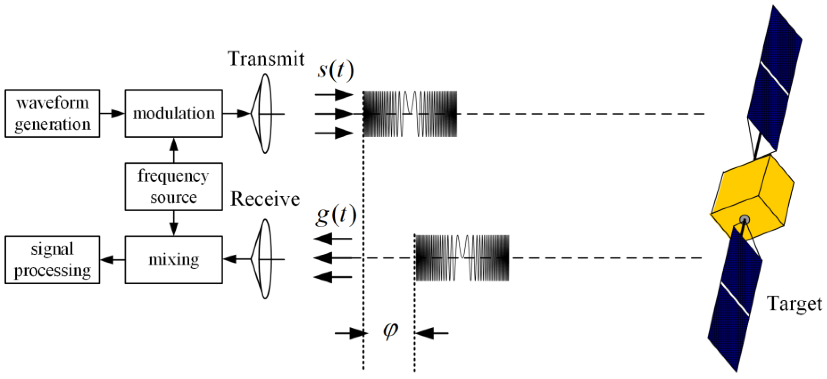
2. Imaging Mechanism of Broadband THz Radars

Broadband THz radar imaging is essentially an active imaging technique that utilizes signal coherence technology to extract Doppler information from the phase variation in the echo signal at THz frequencies, enabling measurement and imaging processing. The working principle of a wideband radar is shown in Figure 1.
The two-dimensional resolution of broadband THz radars is achieved through angle diversity and frequency diversity. Specifically, angle diversity is manifested through relative motion, where the Doppler information resulting from the angular rotation of the target during the coherent integration time (CIT) provides azimuth resolution. Being in the THz frequency range makes the radar more capable of achieving a high resolution under a small angle rotation. On the other hand, frequency diversity is reflected in the broadband spectrum signal. The echoes of objects at different distances occupy different frequency points in the frequency domain, and the wide bandwidth of the modulation signal achieves range resolution.
There are many forms of broadband transmission signals, and here we take the linear frequency modulation (LFM) signal as an example. Let the carrier frequency signal be e j 2 π f c t , the pulse signal is transmitted sequentially with a period T , slow time t m = m T ( m = 0 , 1 , 2 ) , and fast time t ^ = t m T . The transmitted LFM signal can be expressed as Equation (1).
s ( t ^ , t m ) = rect ( t ^ T p ) rect ( t m T a ) exp ( j 2 π ( f c t ^ + 1 2 γ t ^ 2 ) )
where rect ( u ) is the rectangular window function, f c is the center frequency, T p is the sweep time, T a is the total time, γ is the chirp rate, and the bandwidth B = γ T p .
After being reflected by the target, the received signal can be regarded as the superposition of the scattering from individual scattering points on the target, and can be expressed as Equation (2).
s r ( t ^ ) = i = 1 n rect ( t ^ 2 R i / c T p ) rect ( t m T a )   Ω i exp ( j 2 π ( f c ( t 2 R i c ) + 1 2 γ ( t ^ 2 R i c ) 2 )
where R i represents the distance to the ith scattering point, c is the speed of electromagnetic wave propagation, and Ω i represents the scattering coefficient of the ith scattering point in the determined direction.
The demodulated beat signal of the received signal is shown in Equation (3).
s ( t ^ , t m ) = i = 1 n rect ( t ^ 2 R i / c T p ) rect ( t m T a )   Ω i exp ( j 4 π γ c 2 R i 2 ) exp ( j 4 π ( f c + γ t ^ ) R i c )
Under the conditions of the turntable model shown in Figure 2, the instantaneous distance between the scattering point at ( x , y ) and the radar can be expressed as Equation (4).
R ( t ) = r ( t ) + x sin θ ( t ) + y cos θ ( t )
After residual video phase (RVP) compensation, the signal under the small angle approximation can be expressed as Equation (5).
s ( f , t m ) = exp ( j 4 π f c r ( t m ) ) i = 1 n rect ( f f c B ) rect ( t m T a )   Ω i exp ( j 2 π 2 f θ ( t m ) c x i ) exp ( j 2 π 2 f c y i )
After range compression, motion compensation, and azimuth compression, the two-dimensional image I ( x , y ) can be expressed as Equation (6).
| I ( x , y ) | = i = 1 n Ω i 2 Δ B c sin c ( 2 B c ( y y i ) ) 2 f c Δ θ c sin c ( 2 f c Δ θ c ( x x i ) )
It can be summarized from Equation (6) that the range resolution Δ y is c / ( 2 B ) and the azimuth resolution Δ x is c / ( 2 f c Δ θ ) . Δ θ represents the accumulated change in the azimuth angle of the target relative to the radar during the imaging time. As indicated by the resolution formulas, the range resolution of an image depends on the bandwidth. The greater the radar bandwidth, the higher the range resolution. On the other hand, the azimuth resolution of an image depends on the radar center frequency and the rotation angle. When the rotation angle is fixed, the higher the center frequency, the higher the azimuth resolution. Therefore, a terahertz radar can theoretically achieve higher image resolution compared with traditional wavebands.

3. THz Scattering Properties

The high-frequency electromagnetic method under mathematical approximation, as a common physical optics approach, can be used for the scattering characterization calculation of THz waves. In the absence of measured THz scattering data for a material, the Kirchhoff approximation and scalar approximation methods from physical optics can be used to derive the material’s THz scattering coefficient. The bidirectional reflectance distribution function (BRDF) is a commonly used method for characterizing scattering properties in optics. Based on the definition of BRDF and its relationship with the scattering coefficient, THz-BRDF distribution data can be obtained. Borrowing the method for constructing a multi-parameter BRDF model in optics, the multi-parameter THz-BRDF model can be fitted using the distribution data, which enables fast calculation.

3.1. Scattering Coefficient Calculation Based on the Kirchhoff Approximation

The Kirchhoff approximation is suitable for solving the scattered field distribution on the rough local tangent plane. The electromagnetic scattering field under the Kirchhoff approximation is expressed as Equation (7).
E s = K k r S 0 ( n × E Z 0 k r × ( n × H ) ) exp ( j k 1 r ( k r k i ) d S
where K = j k 1 exp ( j k 1 R ) / ( 4 π R ) , k 1 = 2 π / λ is the incident wavenumber, and R represents the distance between the emitting source and the surface element. k r and k i represent the polarization direction vectors of the scattered and incident waves. Z 0 is the intrinsic impedance and n is the unit normal vector of the surface element.
The phase factor Q of Equation (7) can be expressed as Equation (8).
Q = j k 1 r ( k r k i ) = q x x + q y y + q z z
where θ s and θ i represent the incidence angle and scattering angle, respectively, and the other variables are expressed as Equation (9).
{ k s = x sin θ s cos φ s + y sin θ s sin φ s + z cos θ s k i = x sin θ i cos φ i + y sin θ i sin φ i z cos θ i q x = k 1 ( sin θ s cos φ s sin θ i cos φ i ) q y = k 1 ( sin θ s sin φ s sin θ i sin φ i ) q z = k 1 ( sin θ s + sin θ i )
The surface roughness and autocorrelation length are denoted as σ and l , respectively. For surfaces with ( q z σ ) 2 less than about 4, both coherent and incoherent scattering can occur [26].
Under the scalar approximation assumption, the total scattering coefficient σ p q r is as follows:
σ p q r = σ p q c r + σ p q n r + σ p q s r
The coherent scattering coefficient σ p q c r is expressed as Equation (11).
σ p q c r = π k 1 2 | a p q | 2 exp ( q z 2 σ 2 ) δ ( q x ) δ ( q y )
where δ ( x ) is the Dirac function and a p q , p q = HH , VH , VV , HV represent the polarization coefficient [26].
The incoherent scattering coefficient σ p q c r for an isotropic rough surface is expressed as Equation (12).
σ p q n r = ( | a p q | k 1 l / 2 ) 2 exp ( q z 2 σ 2 ) n = 1 ( q z 2 σ 2 ) n ( n ! n ) exp ( ( q x 2 + q y 2 ) l 2 4 n )
The incoherent scattering coefficient σ p q s r caused by the slope of the surface is expressed as Equation (13).
σ p q s r = ( k 1 σ l ) 2 ( q z / 2 ) exp ( q z 2 σ 2 ) Re { a 0 ( q x a 1 * + q y a 2 * ) }   × n = 1 ( q z 2 σ 2 ) n 1 ( n ! n ) exp ( ( q x 2 + q y 2 ) l 2 4 n )

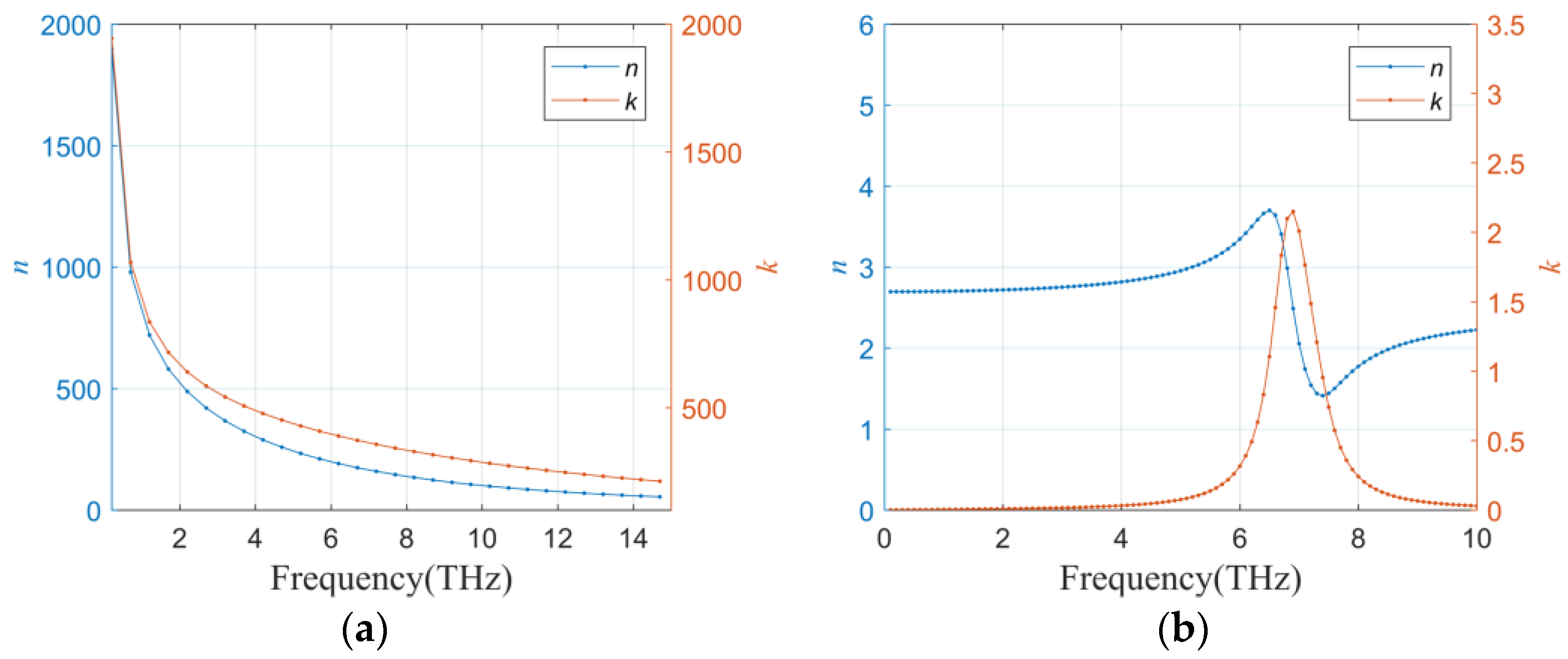
3.2. Complex Refractive Index Calculations

The calculation of scattering coefficients requires the complex refractive index of the material. When the complex refractive index of a material is unknown, it can be calculated from the complex dielectric parameters. Empirical models are commonly used to estimate the complex dielectric parameters for materials that are difficult to measure or have unknown values at a specified frequency in the electromagnetic spectrum. The Drude model is suitable for metals and the Lorentz oscillator model is suitable for dielectric materials.
The Drude model [23] is expressed as Equation (14).
ε r ( ω ) = 1 ω p 2 ω 2 + γ 0 2 ,   ε i ( ω ) = ω p 2 γ 0 ω 3 + ω γ 0 2
The Lorentz oscillator model [23] is expressed as Equation (15).
ε ( ω ) = ε ( ) ( 1 + ω L O 2 ω T O 2 ω T O 2 ω 2 + i ω r )
The complex refractive index n ˜ = n + i κ of a material can be calculated based on its complex dielectric parameters, expressed by Equation (16).
n ( ω ) = ( ε r ( ω ) + ε r 2 ( ω ) + ε i 2 ( ω ) ) / 2 κ ( ω ) = ( ε r ( ω ) + ε r 2 ( ω ) + ε i 2 ( ω ) ) / 2
Aluminum (Al) metal and white-painted Al are used as examples. According to relevant literature [23,27], the Drude model‘s parameters of Al are set to ω p = 3435.6 and γ 0 = 8.0 , and the Lorentz oscillator model’s parameters of white-painted Al are set to ε ( ) = 5.996 , ω L O = 7.44 , ω T O = 6.76 , and r = 0.67 . The variation in the complex refractive index with frequency for the two materials is shown in Figure 3.
Figure 3a,b depicts the variations in the complex refractive index’s real and imaginary parts for Al and white-painted Al in the frequency range of 0.2 to 15 THz. Within each sub-figure, the blue line represents the real part n , while the red line represents the imaginary part κ . At a frequency of 0.215 THz, the complex refractive index of several materials can be obtained based on the empirical models of the complex dielectric parameters and relevant literature [28], as shown in Table 1.

3.3. Multi-Parameter THz-BRDF Model Construction

With reference to the definition of the bidirectional reflectance distribution function (BRDF) in optics, BRDF of a radar is defined as Equation (17).
f r = P r P s cos θ r d Ω
where P s and P r represent the incident power and scattered power, respectively; θ r is the scattering angle; and d Ω is the solid angle.
According to the definition of the scattering coefficient, the relationship between the scattering coefficient and BRDF can be expressed as Equation (18).
d σ = 4 π R 2 P s P i = 4 π f r cos θ i cos θ r d S
The total scattering coefficient (RCS) of all irradiated parts in the area S 0 can be expressed as Equation (19).
σ = S 0 4 π f r cos θ i cos θ r d S
In the field of optics, there have been many studies on the construction method and fitting method of the material BRDF model [29,30], among which the multi-parameter BRDF model improved based on the Torrance sparrow model [30,31] is common. The expression of the multi-parameter BRDF model is as follows:
f r = k b D F G cos θ r + k d
where D is the normal distribution function of the microfacet, F is the Fresnel reflection coefficient, G is the geometric attenuation factor, and k d is the diffuse reflection coefficient.
The improved six-parameter model [32] that satisfies energy reciprocity after the above model is expressed as follows:
f r = k b π ln 2 k r 2 cos α 1 + ( k r 2 1 ) cos α exp [ | b | ( 1 cos γ ) a ]   × ln ( 1 + cos θ i cos θ r ) + k d π ( cos θ i cos θ r ) c
where k b , k r , b , a , k d , and c are the six parameters of the BRDF model.
The angle relationships in Equation (21) are expressed as Equation (22).
{ cos α = cos θ i + cos θ r 2 cos γ cos γ = ( cos θ i cos θ r + sin θ i sin θ r cos ϕ + 1 ) / 2
where i and r represent incidence and reflection, respectively, and θ and ϕ represent the zenith angle and azimuth angle, respectively.
The definition of fitting error of the multi-parameter BRDF model can be expressed as Equation (23).
e = θ i θ r [ f r model cos ( θ r ) f r 0 cos ( θ r ) ] 2 θ i θ r [ f r 0 cos ( θ r ) ] 2
where f r model represents the fitting BRDF value, f r 0 represents the theoretically calculated BRDF value, and θ r is the scattering angle.
According to the complex refractive index values n ˜ in Table 1, along with the set surface roughness σ and autocorrelation length l , the scattering coefficient and BRDF of the material can be calculated using Equations (10)–(13) under an incident zenith angle of 30~60°, scattering zenith angle of −40~80°, and azimuth angle of 180°. Using the calculated four-dimensional data points of the incident zenith angle, scattering zenith angle, and azimuth angle, and BRDF as input, a BP neural network is utilized to iteratively estimate the model parameters by setting the initial parameters and updating them in the direction of gradient descent until a predetermined error range is reached, and the fitted model parameters are obtained. The theoretical simulation results and fitted model results of BRDF for the three materials are shown in Figure 4.
The fitting parameters and error results of the six-parameter BRDF model are shown in Table 2.
The fitting results enable the provision of target scattering characteristics in the radar echo simulation process. Considering the ongoing challenge of acquiring real THz scattering characteristic data [22], the fitted data utilized in this study are based on theoretical data obtained using the Kirchhoff approximation method, which has been widely recognized in the industry [26,27] for its feasibility in solving scattering coefficients. The above fitting results have credibility and reference value in practical application.

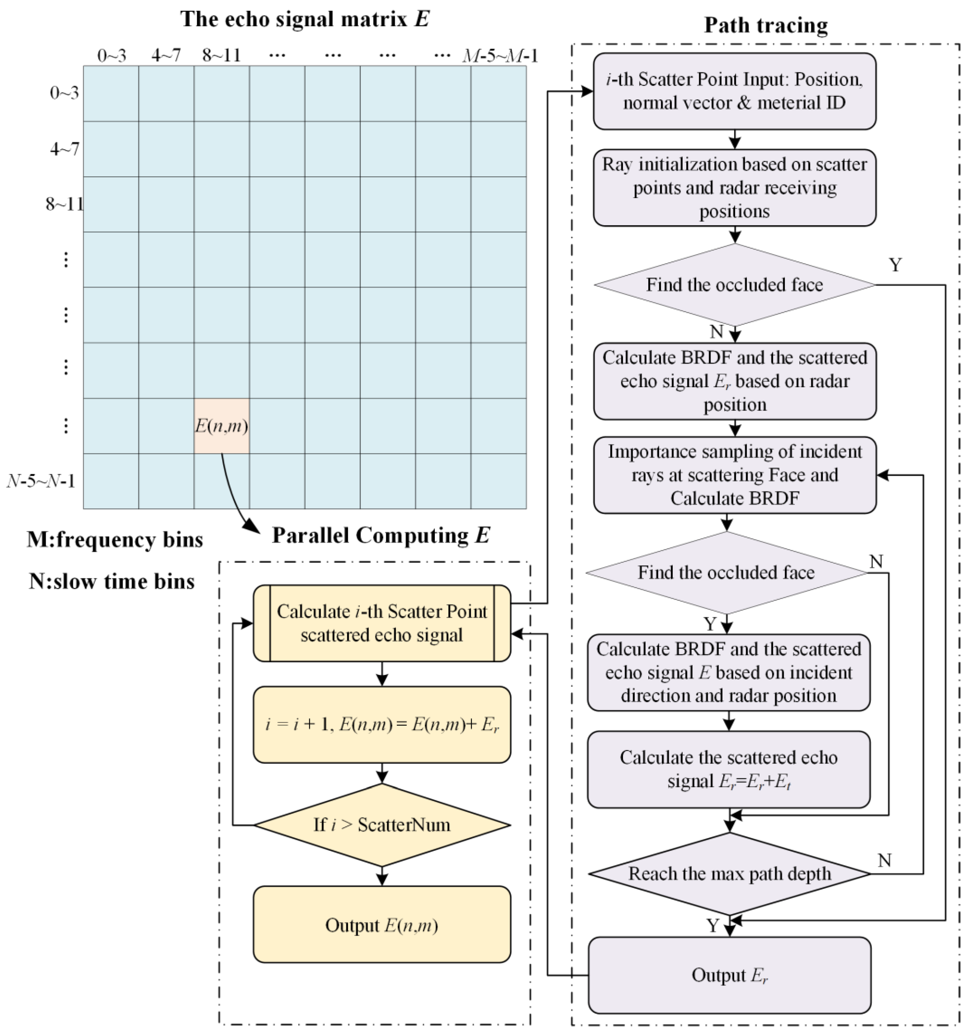
4. THz Radar Imaging Simulation Based on the Improved Path Tracing Algorithm

The path tracing algorithm is a common computational method used in physics-based image rendering. According to the working mechanism of broadband terahertz radar imaging, an improved path tracing algorithm suitable for simulating THz radar raw echo data is proposed in this paper. Based on the classical backscattering model, the improved path tracing algorithm for THz radars proposed in this paper utilizes parallel threads to rapidly calculate the attenuation and accumulation of multi-path scattering energy, leading to a more accurate simulation of the radar echo data. Moreover, compared with the general path tracing rendering method, we add a phase factor related to the path length in the process of calculating the backscattering signal. Furthermore, when calculating the scattered energy, we use the BRDF model from the previous section to determine the scattering coefficient at the incident and reflect angles.
Path tracing is the process by which rays emitted from the transmitter travel through a series of paths before reaching the receiver. The paths may include primary or multiple reflections, as illustrated in Figure 5.
The echo data matrix to be generated is a two-dimensional data matrix consisting of M frequency points and N slow time points. Based on the independence of data at each frequency point and slow time point, the data for each grid point can be calculated in parallel. Considering any grid point E(n, m) as an example, the data at this grid point are obtained by accumulating the echo signals from all of the contributing scattering points. The flow chart of the improved path tracking algorithm is shown in Figure 6. The procedure for calculating each scattering point is as follows.
Step 1: First, initialize the ray based on the position of the scattering point P n and the antenna. Use bounding boxes to determine if the ray is occluded by triangle facets. If the scattering point is visible, the scattering coefficient Ω 0 is calculated based on the incident and exit directions of the ray (both pointing towards the antenna from the scattering point). The primary scattered echo signal E r (at i = 0 in Equation (27)) is calculated.
Step 2: After completing the single backscatter calculation as described above, multiple iterations of scattering paths are performed. Importance sampling of scattering direction is carried out based on the radar incidence direction at the initial scattering point, and the scattering coefficient Ω 1 is calculated for this direction.
Step 3: Update the direction of the ray, and check if the scattered ray intersects with the triangle facets. If not, exit the loop. If there is an intersection point P n + i , the scattering coefficient Ω i ( i > 1 ) is calculated based on the incident direction of the light ray and the direction towards the antenna at the intersection point. The multiple scattered echo signal E t (the part added for the i-th iteration in Equation (27)) is calculated and added to the above signal E r = E r + E t .
Step 4: Update the scattering coefficient Ω i and the path total distance l = n n + i ( R P l 1 P l ) , iterate Step 3 until reaching the maximum path depth K , and output the total echo signal E r of the scattering point P n .
The scattering coefficient calculation process in the above steps can be summarized in a recursive form, as shown in Equations (24)–(26).
W n = σ L P n P n + 1 ( 4 π R P n P n + 1 2 ) PDF L P n P n + 1 = 4 π f L P n P n + 1 cos ( θ L P n ) cos ( θ P n P n + 1 ) d S ( 4 π R P n P n + 1 2 ) PDF L P n P n + 1
W n + k = W n + k 1 σ P n + k 1 P n + k L ( 4 π R P n + k L 2 ) PDF P n + k 1 P n + k L = ( i = n n + k σ P i 1 P i P i + 1 4 π R P i P i + 1 2 PDF P i 1 P i P i + 1 )
Ω k = W n + k A e 4 π R P n + k L 2
where W n represents an intermediate variable; W n + k means W n iterates to the k-th time; Ω k represents the total scattering coefficient factor for k paths; σ represents the scattering coefficient and f represents the corresponding BRDF; PDF represents the probability distribution function; R represents the length of the path; P n + k represents the starting scatter point of the k-th path; L represents the radar itself; P i 1 P i P i + 1 represents the path from P i 1 to P i , and then from P i to P i + 1 , particularly, P n 1 , P n + k + 1 L ; and A e represents the effective antenna aperture.
Considering the scattering coefficient factors Ω i and phase factors ϕ i related to the total length of each path, the echo signal formula is expressed as follows:
E r = 1 N i ray = 1 N ( i = 0 K ( P s G R Ω i 4 π R P n L 2 ) 1 2 exp ( j ϕ i ) ) ,   ϕ i = 2 π f m l = n n + i ( R P l 1 P l ) c
where N represents the number of rays, K represents the path depth, P s represents the radar transmit power, G R represents the antenna gain, and f m represents the m-th frequency point.
All surface element scattering centers are traversed to calculate the echo signal E(n, m) at the m-th range bin and the n-th received pulse. The final echo signal data are composed of an N × M matrix. To obtain the two-dimensional image, the echo signal data are subject to range-Doppler (R-D) processing. Firstly, the range profiles are obtained by applying the FFT to the echo data matrix. Then, the range profiles are aligned using the minimum entropy method. Next, the phase correction is applied based on phase gradient autofocus (PGA) [33]. Finally, the two-dimensional R-D image is generated applying the FFT to the data after motion compensation.

5. THz Radar Imaging Simulation Experiment and Discussion

5.1. Simulation Input Conditions

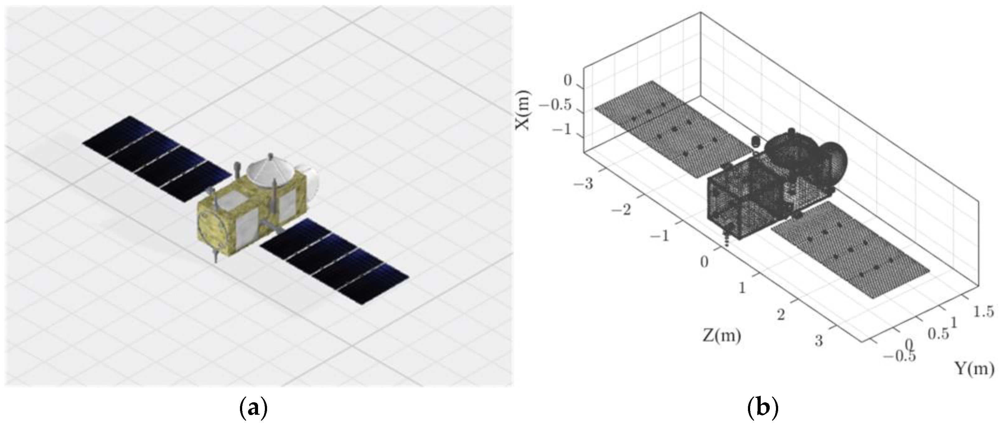
5.1.1. Geometric Processing of the Target 3D Model

The scatter point distribution matching the spatial resolution ability is obtained through the finite element partition of the target 3D model. Taking the Jason-1 satellite model as an example, 119,110 scattering points are obtained after subdivision. The schematic diagram of the 3D model is shown in Figure 7.
During the subdivision process, we differentiated all scattering points based on their corresponding components and materials, as presented in Table 3. The division of materials can provide a basis for using different BRDF models in the subsequent simulation process. Owing to the uncertain characteristics of materials such as solar cells on the satellite panel, the current simulation employs aluminum plates (without attached solar cells), which are commonly used in most indoor validations. In the future, we will conduct further research on the scattering characteristics of solar cells to achieve more precise results.

5.1.2. THz Radar Parameters

According to the THz radar design index in engineering applications, the simulation parameters of the THz radar are shown in Table 4. According to Equation (6), the range resolution is 1.5 cm.

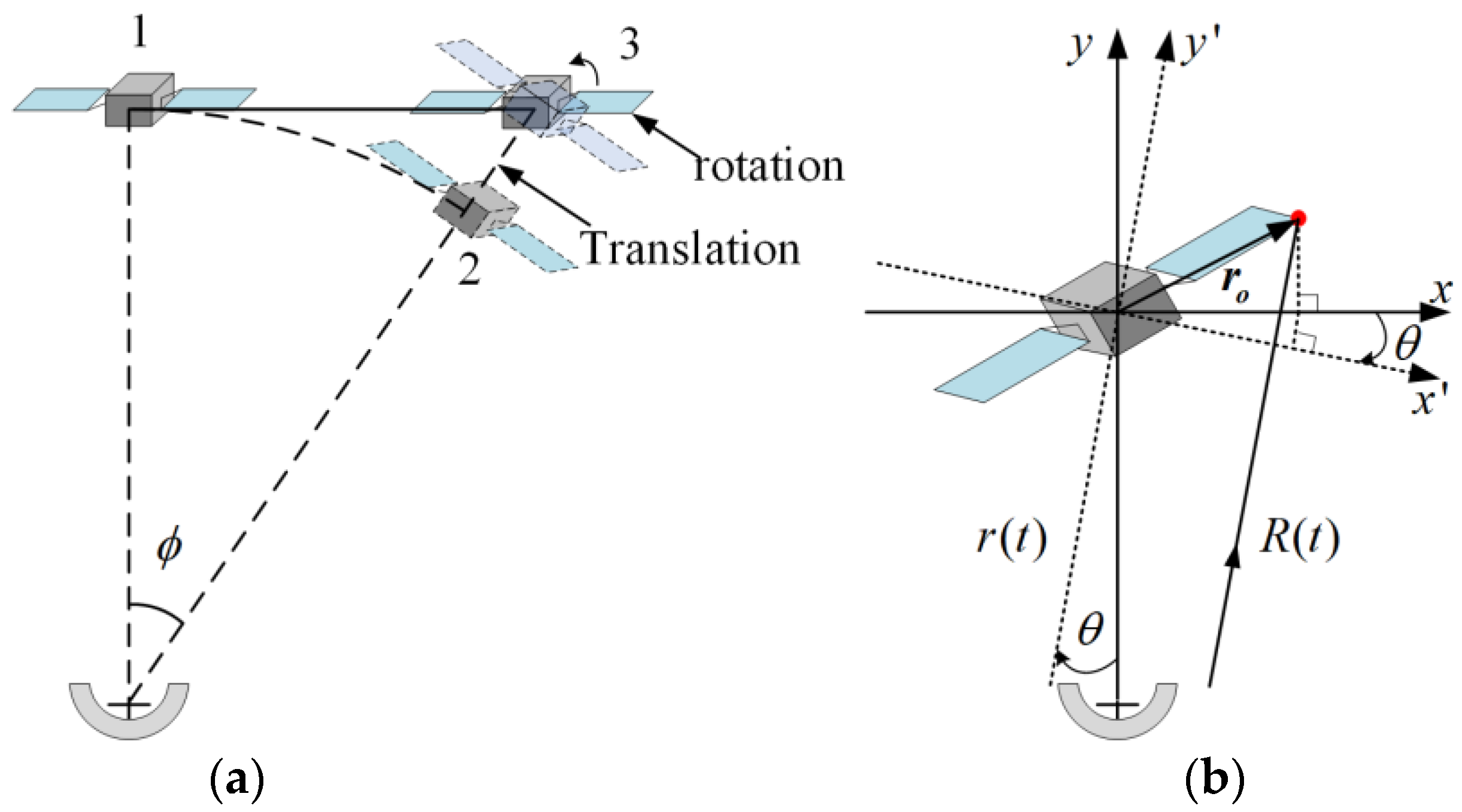
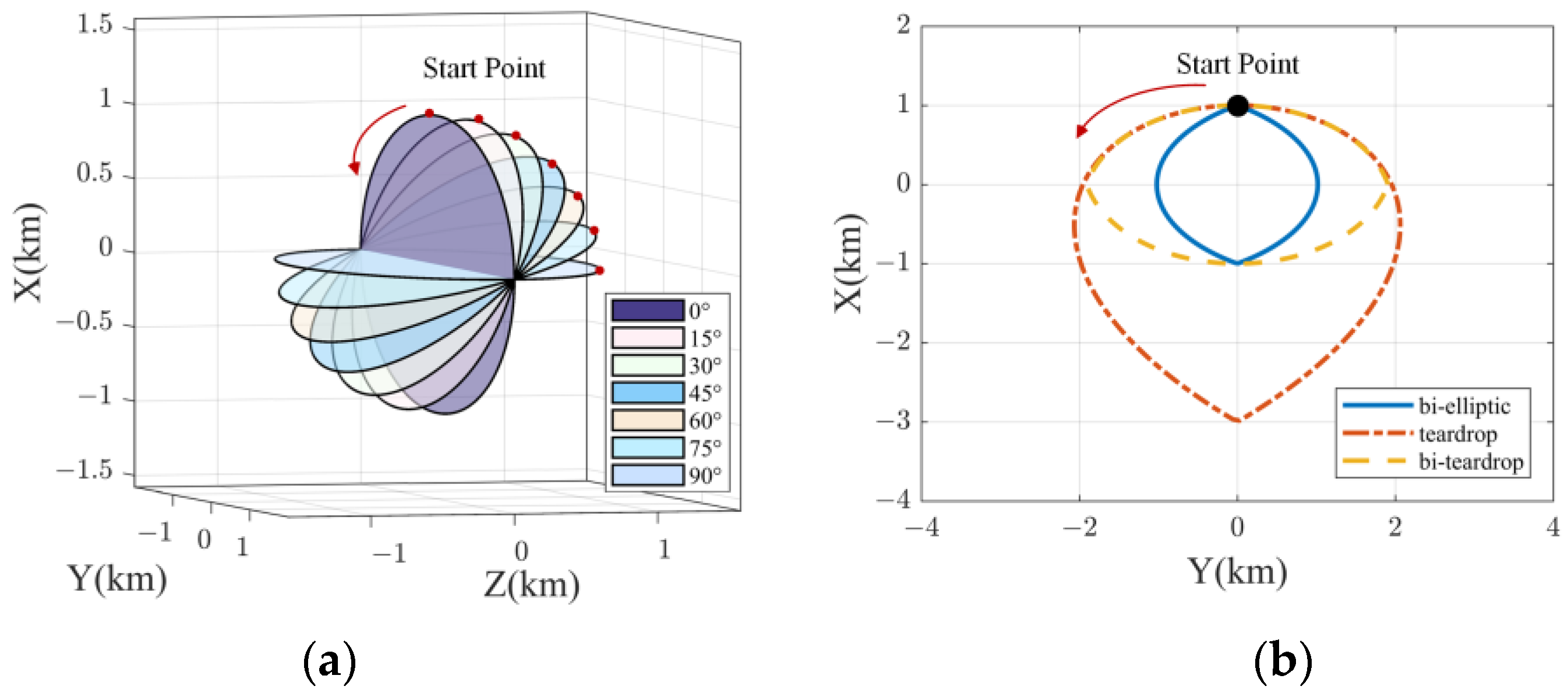
5.1.3. On-Orbit Relative Motion Model

The imaging mechanism of a space-based terahertz radar determines that its imaging process has certain requirements for the relative motion relationship between the target and the accompanying spacecraft. The presence of azimuthal angle variations is essential to obtain the azimuthal (cross-range) resolution in the radar imaging process. The in-orbit fly-around motion satisfies the above requirements well. Therefore, this paper focuses on analyzing the relative motion relationship under several typical fly-around formations.
The fly-around motion can be classified into natural and forced fly-around based on whether the process has external forces. This paper considers natural fly-around with an interval of 15° between 0° and 90° inclination to the target orbital plane and forced fly-around such as bi-ellipse, teardrop, and bi-teardrop fly-around with 0° inclination. By establishing the LVLH coordinate system O-XYZ with the target’s center of mass as the origin (Figure 8a), the relative motion model between spacecraft is constructed according to the C-W equation (Hill equation). The analytical solutions for different fly-around formations can be obtained by setting the initial state and the mid-course control pulse of the accompanying spacecraft [34]. It is assumed that the target orbit is a circular orbit with a semi-major axis of 1000 km and an orbital period T of approximately 6298 s. Natural fly-around has the same period T 0 = T as the target orbit, while the forced fly-around period is set to T 1 = 0.6 T . The trajectories of fly-around formations are shown in Figure 9. The motion is counterclockwise, and the starting point is at the maximum X-coordinate (the maximum Z-coordinate in 90° natural fly-around) where the trajectory intersects with the Y = 0 plane.

5.2. Effects on Imaging Process of Different Fly-Around Formations

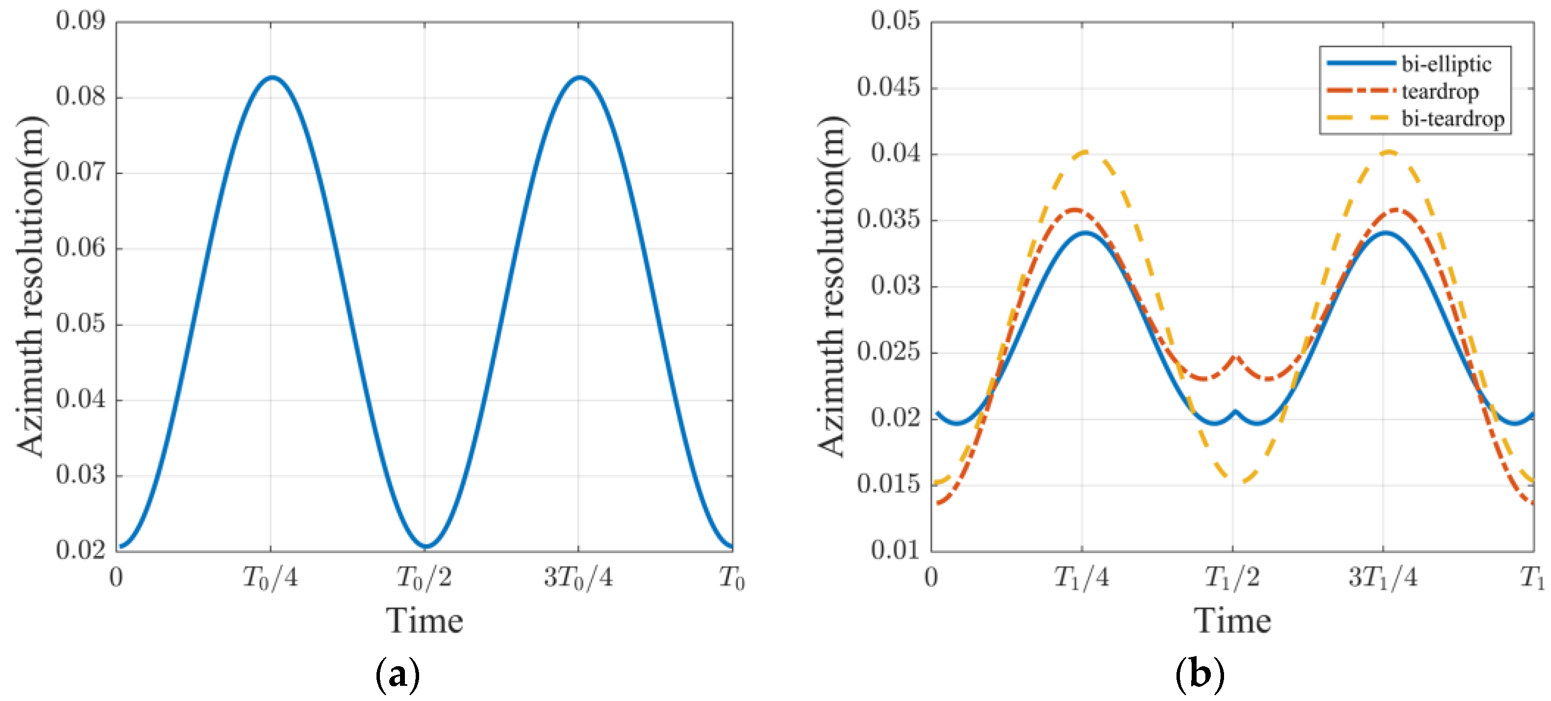
5.2.1. Azimuth Resolution

Based on the fly-around trajectory and radar parameters, the rotational angle change can be calculated for each coherent integration time, enabling the determination of azimuth resolution variations during different observation time intervals within one fly-around period. The results are shown in Figure 10. T 0 and T 1 in the figure represent the periods of natural fly-around and forced fly-around, respectively. For a fixed observation time, the azimuthal resolutions for natural fly-around with different inclinations remain below 9 cm, with an optimal scale of 2 cm. The azimuth resolutions of the forced fly-around are below 4 cm, with an optimal value of approximately 1.3 cm. Owing to its shorter period, the forced fly-around exhibits larger angular rotation within the same observation time, thus enabling higher azimuth resolution. The azimuth resolutions remain within the same order of magnitude as the 1.5 cm range resolution, facilitating two-dimensional imaging.

5.2.2. RCS

For each fly-around formation, considering the relative positions of the targets and accompanying spacecraft within one period, the RCS of the entire satellite can be obtained by summing up the RCS contributions from each visible facet using Equation (19). The results are shown in Figure 11.
From Figure 11, it can be observed that different fly-around formations exhibit a consistent overall trend, yet still display local differences. Figure 11a shows that, under the natural fly-around with inclinations ranging from 0 to 90 degrees, the RCS peak initially decreases and then increases. The peak RCS value reaches a maximum of 19.2 dBsm in a 0° natural fly-around, while the minimum RCS value reaches −17.2 dBsm in a 45° natural fly-around. Figure 11b shows that the RCS changes of the three kinds of forced fly-around formations with 0° inclination are similar to the 0° natural fly-around, yet there are some slight differences in the local positions.

5.2.3. Range Migration

Under different fly-around formations, the range profiles of the echo signal after pulse compression will produce various range migrations, which will have an impact on the selection of motion compensation methods. Owing to the similar pattern of range migration variation for natural fly-around at different inclinations, 0° natural fly-around and bi-ellipse, teardrop, and bi-teardrop forced fly-around are selected for comparison. In one fly-around period, the range migrations produced by different fly-around methods during each observation period are illustrated in Figure 12. The figure on the left side of each change curve presents the range profile of its 13th frame.
From the results in Figure 12, it can be observed that the range migrations differ significantly among the various fly-around formations. In the slow-time domain, the range migration of a single frame generally follows a first- or second-order curve. By utilizing the minimum entropy method to estimate the velocity and acceleration of the motion, effective translational compensation can be achieved, resulting in range profile alignment.

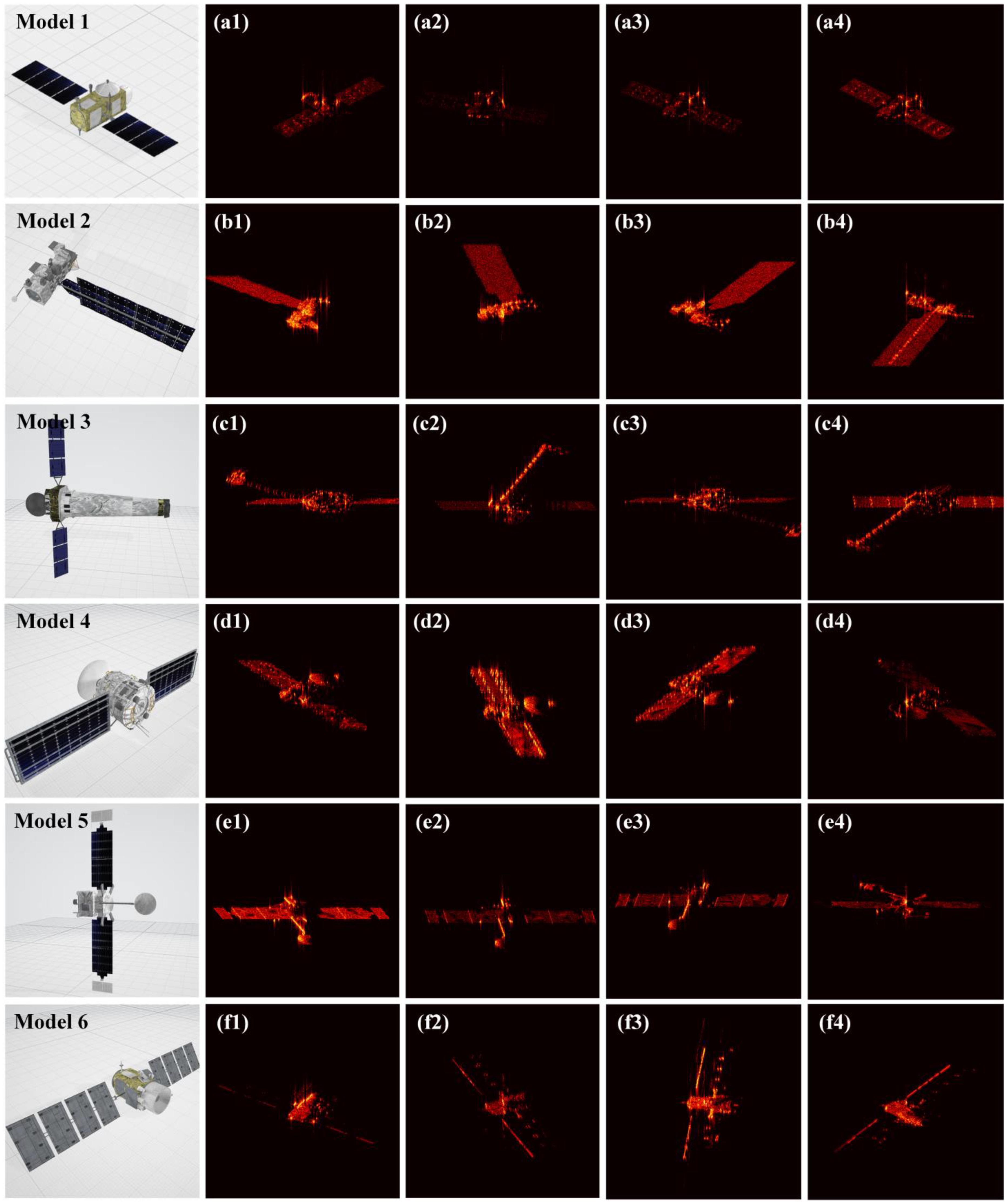
5.3. The Results of Imaging Simulation

5.3.1. Results for a Single Frame

Based on the improved path tracing THz radar imaging simulation method described in Section 4, with the path depth set to 3, the simulated echo signals are generated using the relative motion pose of a 45° natural fly-around as input. The echo signals are subjected to range compression, range profile alignment, and phase correction. Taking the observation data within the fifth frame as an example, the results of each imaging stage in the coherent integration time are shown in Figure 13.
To perform a quantitative analysis of the results, the effectiveness of range profile alignment can be compared using the entropy function H 0 defined by Equation (28), where S n represents the nth range profile. Similarly, the effectiveness of PGA can be compared using the entropy function H defined by Equation (29), where S m n represents the pixel values. The meaning of the entropy functions is that, the smaller the value, the better the quality of the result.
H 0 ( S n ) = n = 1 N p ( n ) log { p ( n ) } ,   p ( n ) = S n S n + S 1
H ( S m n ) = m = 1 M n = 1 N p ( m , n ) log { p ( m , n ) } ,   p ( m , n ) = S m n m = 1 M n = 1 N S m n
From the result shown in Figure 13a, it can be observed that there is range migration in the on-orbit THz radar imaging. Figure 13b and Figure 14a show that effective range profiles alignment can be achieved utilizing the minimum entropy method. Figure 13c and Figure 14b show that using the phase gradient autofocus (PGA) algorithm on the aligned range profiles yields well-focused two-dimensional images.

5.3.2. Comparison and Discussion

To demonstrate the advantages of the simulation method proposed in this paper, a comparison was conducted with the widely-used fast-physical optics (FPO) method [35,36,37] under identical imaging conditions (see Section 5.3.1) and the same satellite model (see Section 5.1.1). Figure 15 shows the comparison of the simulation results of the 10th, 15th, and 20th frames in fly-around imaging. The graphs in each column (such as Figure 15a1,a2) correspond to the same observation conditions. The disparities in target positions arise from variations in the extremal points selected during the image-focusing algorithm process. As this does not impact the comparative analysis, no additional alignment processing was undertaken. By comparing the results on individual frames, we observe two key aspects. On the one hand, owing to the THz-BRDF scattering model, the scattering characteristics of the antenna and connector are more pronounced in our results. On the other hand, by employing multi-path tracing, our approach effectively captures local multiple scattering phenomena, thus better aligning with real-world behaviors. These two aspects are the main differences between our method and the FPO method.
To further quantitatively compare and analyze the results of the two methods, we first convert the image data into grayscale and then utilize several indicators for the comparative assessment of the target regions, including grayscale mean, grayscale variance, and entropy. The formulas for grayscale mean and grayscale variance are commonly known and require no further elaboration. The formula for entropy is expressed as Equation (29). The quantitative comparison results between the two methods are presented in Table 5.
The results presented in Table 5 reveal two main observations. Firstly, our method exhibits lower grayscale mean under the same intensity scale. This is because the FPO method we use does not consider real scattering coefficients and assumes a constant amplitude of 1. In contrast, our method calculates the echo energy based on THz scattering characteristics, resulting in relatively lower energy in local regions, which better meets the requirements for analyzing the signal-to-noise ratio in practical systems. Moreover, our method shows larger grayscale variance, indicating that it captures richer local details. Secondly, the entropy value indicates a slightly higher value in our results compared with the other method. We attribute this to the mild defocusing caused by multiple-path scattering. Despite a slight decline in the image’s focusing quality compared with ideal conditions, it facilitates a more faithful representation of real-world scenarios and proves advantageous for validating various radar image processing algorithms.

5.3.3. Dataset Results

Compared with the limited quantity of available measurement data, simulation methods provide a fast and efficient way to obtain a wealth of results. The THz radar image dataset based on simulated data can serve as input for various deep-learning-based detection and recognition algorithms. Taking six satellite models as an example, we present a selection of images from the dataset in Figure 16, generated under different azimuth angles and a fixed elevation of 45° (definition in Figure 8b) during a fly-around. From Figure 16, it can be observed that there are inconsistencies in the image-focusing performance under different viewing angles. Therefore, it is necessary to further optimize the motion compensation process for the fly-around.

6. Conclusions

To address the issue of severe image scarcity in the ground test of space-based THz radars, we proposed a simulation method for THz radar imaging based on improved path tracing according to the imaging mechanism of broadband THz radars. Firstly, the characterization method of THz scattering properties was presented based on physical optics, which is used in cases where THz measurement data are lacking. The multi-parameter THz-BRDF models of aluminum, white-painted Al, and polyimide film at 0.215 THz were fitted based on theoretical data, with fitting errors below 4%. Then, the THz radar imaging simulation method based on improved path tracing was presented in detail. The simulation method utilizes path tracing to simulate THz radar echo signal data, considering phase factors related to path length and multi-path energy scattering based on the THz-BRDF model. The echo signals are processed using the range-Doppler technique to achieve two-dimensional imaging. Finally, we conducted THz radar imaging simulation experiments. The influences in the imaging process of different motion models, including natural fly-around, bi-ellipse forced fly-around, teardrop forced fly-around, and bi-teardrop forced fly-around, were analyzed from several aspects: azimuth resolution, RCS, and range migration. A comparison was conducted with the FPO method, and the comparative results indicate the feasibility and advancement of the proposed method. The simulation results can serve as a data source for the ground test of space-based THz radars, particularly in the evaluation of target detection and recognition algorithms based on deep learning, providing strong support for the application of space-based THz radars in the future.

Author Contributions

Conceptualization, H.W.; Formal analysis, Q.N.; Funding acquisition, H.W.; Investigation, Q.N., Z.Y. and X.L.; Methodology, Q.N.; Project administration, H.W.; Software, Q.N.; Supervision, H.W.; Validation, Q.N., Z.Y. and Y.L.; Visualization, Q.N., Z.Y. and X.L.; Writing—original draft, Q.N.; Writing—review and editing, Q.N. All authors have read and agreed to the published version of the manuscript.

Funding

This research was funded by the National Natural Science Foundation of China, grant number 61705220.

Institutional Review Board Statement

Not applicable.

Informed Consent Statement

Not applicable.

Data Availability Statement

Not applicable.

Acknowledgments

We sincerely thank the National Natural Science Foundation of China for its support.

Conflicts of Interest

The authors declare no conflict of interest.

References

  1. Scott, R.; Thorsteinson, S. Key Findings from the NEOSSat Space-Based SSA Microsatellite Mission. In Proceedings of the Advanced Maui Optical and Space Surveillance Technologies Conference, Maui, HI, USA, 11–14 September 2018; Available online: www.amostech.com (accessed on 26 May 2023).
  2. Ender, J.; Leushacke, L.; Brenner, A.; Wilden, H. Radar techniques for space situational awareness. In Proceedings of the 2011 12th International Radar Symposium (IRS), Leipzig, Germany, 7–9 September 2011; pp. 21–26. [Google Scholar]
  3. Yunpeng, H.; Kebo, L.; Yan’gang, L.; Lei, C. Review on strategies of space-based optical space situational awareness. J. Syst. Eng. Electron. 2021, 32, 1152–1166. [Google Scholar] [CrossRef]
  4. Speretta, S. Space Surveillance Network Capabilities Evaluation Mission. In Proceedings of the 2nd NEO and Debris Detection Conference, Darmstadt, Germany, 24–26 January 2023; Available online: https://conference.sdo.esoc.esa.int/proceedings/neosst2/paper/127/NEOSST2-paper127.pdf (accessed on 26 May 2023).
  5. Czerwinski, M.G.; Usoff, J.M. Development of the Haystack Ultrawideband Satellite Imaging Radar. Linc. Lab. J. 2014, 21, 28–44. [Google Scholar]
  6. Cerutti-Maori, D.; Rosebrock, J.; Carloni, C.; Budoni, M.; Maouloud, I.; Klare, J. A Novel High-Precision Observation Mode for the Tracking and Imaging Radar TIRA—Principle and Performance Evaluation. In Proceedings of the 8th European Conference on Space Debris (Virtual), ESA/ESOC, Darmstadt, Germany, 20–23 April 2021; Available online: https://conference.sdo.esoc.esa.int/proceedings/sdc8/paper/221/SDC8-paper221.pdf (accessed on 26 May 2023).
  7. Marchetti, E.; Stove, A.G.; Hoare, E. Space-Based Sub-THz ISAR for Space Situational Awareness-Laboratory Validation. IEEE Trans. Aerosp. Electron. Syst. 2022, 58, 4409–4422. [Google Scholar] [CrossRef]
  8. Božanić, M.; Sinha, S. Emerging Transistor Technologies Capable of Terahertz Amplification: A Way to Re-Engineer Terahertz Radar Sensors. Sensors 2019, 19, 2454. [Google Scholar] [CrossRef] [Green Version]
  9. Valušis, G.; Lisauskas, A.; Yuan, H.; Knap, W.; Roskos, H.G. Roadmap of Terahertz Imaging 2021. Sensors 2021, 21, 4092. [Google Scholar] [CrossRef] [PubMed]
  10. Zhang, Y.; Yang, Q.; Deng, B.; Qin, Y.; Wang, H. Estimation of Translational Motion Parameters in Terahertz Interferometric Inverse Synthetic Aperture Radar (InISAR) Imaging Based on a Strong Scattering Centers Fusion Technique. Remote Sens. 2019, 11, 1221. [Google Scholar] [CrossRef] [Green Version]
  11. Wang, M.; Zhong, K.; Liu, C.; Xu, D.; Shi, W.; Yao, J. Optical coefficients extraction from terahertz time-domain transmission spectra based on multibeam interference principle. Opt. Eng. 2017, 56, 044101. [Google Scholar] [CrossRef]
  12. Di Simone, A.; Fuscaldo, W.; Millefiori, L.M.; Riccio, D.; Ruello, G.; Braca, P.; Willett, P. Analytical Models for the Electromagnetic Scattering from Isolated Targets in Bistatic Configuration: Geometrical Optics Solution. IEEE Trans. Geosci. Remote Sens. 2020, 58, 861–880. [Google Scholar] [CrossRef]
  13. Potter, L.C.; Chiang, D.-M.; Carriere, R.; Gerry, M.J. A GTD-based parametric model for radar scattering. IEEE Trans. Antennas Propag. 1995, 43, 1058–1067. [Google Scholar] [CrossRef]
  14. Asvestas, J.S. The physical optics method in electromagnetic scattering. J. Math. Phys. 1980, 21, 290–299. [Google Scholar] [CrossRef]
  15. Tian, G.; Tong, C.; Sun, H.; Zou, G.; Liu, H. Improved Hybrid Algorithm for Composite Scattering from Multiple 3D Objects Above a 2D Random Dielectric Rough Surface. IEEE Access 2020, 9, 4435–4446. [Google Scholar] [CrossRef]
  16. Boag, A. A fast physical optics (FPO) algorithm for high frequency scattering. IEEE Trans. Antennas Propag. 2004, 52, 197–204. [Google Scholar] [CrossRef]
  17. Garcia-Fernandez, A.F.; Yeste-Ojeda, O.A.; Grajal, J. Facet model of moving targets for ISAR imaging and radar back-scattering simulation. IEEE Trans. Aerosp. Electron. Syst. 2010, 46, 1455–1467. [Google Scholar] [CrossRef]
  18. Kulpa, K.S.; Samczynski, P.; Malanowski, M.; Gromek, A.; Gromek, D.; Gwarek, W.; Salski, B.; Tanski, G. An Advanced SAR Simulator of Three-Dimensional Structures Combining Geometrical Optics and Full-Wave Electromagnetic Methods. IEEE Trans. Geosci. Remote Sens. 2014, 52, 776–784. [Google Scholar] [CrossRef]
  19. Wang, F.; Eibert, T.F.; Jin, Y.-Q. Simulation of ISAR Imaging for a Space Target and Reconstruction under Sparse Sampling via Compressed Sensing. IEEE Trans. Geosci. Remote Sens. 2015, 53, 3432–3441. [Google Scholar] [CrossRef]
  20. Chiang, C.-Y.; Chen, K.-S.; Yang, Y.; Zhang, Y.; Zhang, T. SAR Image Simulation of Complex Target including Multiple Scattering. Remote Sens. 2021, 13, 4854. [Google Scholar] [CrossRef]
  21. Wu, K.; Jin, G.; Xiong, X.; Zhang, H.; Wang, L. SAR Image Simulation Based on Effective View and Ray Tracing. Remote Sens. 2022, 14, 5754. [Google Scholar] [CrossRef]
  22. Gao, J.; Deng, B.; Qin, Y. Radar echo scattering modeling and image simulations of full-scale convex rough targets at terahertz frequencies. J. Radars 2018, 7, 97–107. [Google Scholar] [CrossRef]
  23. Mou, Y.; Sheng, X.; Gao, Y. Bidirectional reflection distribution function modeling (BRDF) for terahertz diffuse scattering analysis of dielectric rough targets. Infrared. Phys. Technol. 2019, 101, 171–179. [Google Scholar] [CrossRef]
  24. Marchetti, E.; Stove, A.G.; Hoare, E.G. Space-based Sub-THz ISAR for Space Situational Awareness Concept and Design. IEEE Trans. Aerosp. Electron. Syst. 2021, 58, 1558–1573. [Google Scholar] [CrossRef]
  25. Zhang, Y.; Yang, X.; Jiang, X. Attitude direction estimation of space target parabolic antenna loads using sequential terahertz ISAR images. J. Infrared Millim. Waves. 2021, 40, 496–507. [Google Scholar] [CrossRef]
  26. Ulaby, F.T.; Moore, R.K.; Fung, A.K. Microwave Remote Sensing, Active and Passive: Volume II, Radar Remote Sensing and Surface Scattering and Emission Theory; Artech House: London, UK, 1982; pp. 304–307. [Google Scholar]
  27. Mou, Y.; Wu, Z.S.; Zhang, G.; Gao, Y.Q.; Yang, Z.Q. Establishment of THz dispersion model of metals based on Kramers-Kronig relation. Acta Phys. Sin. 2017, 66, 120202. [Google Scholar] [CrossRef]
  28. Shi, J.H.; Dong, G.H.; Xu, W.X.; Wang, Y.; Sun, M.; Li, Y.; Zhu, Z.; Lubo. Optically controlled Fano resonance in hybrid fishscale metamaterial. J. Terahertz Sci. Electron. Inf. Technol. 2022, 20, 566. [Google Scholar] [CrossRef]
  29. Ding, Z.; Han, Y. Infrared characteristics of satellite based on bidirectional reflection distribution function. Infrared Phys. Technol. 2019, 97, 93–100. [Google Scholar] [CrossRef]
  30. Wang, H.; Chen, Y. Modeling and simulation of infrared dynamic characteristics of space-based space targets. Infrared Laser Eng. 2016, 45, 0504002. [Google Scholar] [CrossRef]
  31. Torrance, K.E.; Sparrow, E.M. Theory for off-specular reflection from roughened surfaces. J. Opt. Soc. Am. 1967, 57, 1105–1114. [Google Scholar] [CrossRef]
  32. Yang, Y.F.; Wu, Z.S.; Cao, Y.H. Practical six-parameter bidirectional reflectance distribution function model for rough surface. Acta Opt. Sin. 2012, 32, 0229001. [Google Scholar] [CrossRef]
  33. Chen, V.C. Inverse Synthetic Aperture Radar Imaging: Principles, Algorithms and Applications; Institution of Engineering and Technology: Stevenage, UK, 2014; pp. 77–94. [Google Scholar]
  34. Zhang, R.; Yin, J.; Han, C. Spacecraft forced fly-around formation design and control. J. Beijing Univ. Aeronaut. Astronaut. 2017, 43, 2030. [Google Scholar] [CrossRef]
  35. Zhou, Y.; Zhang, L.; Cao, Y. Optical-and-radar image fusion for dynamic estimation of spin satellites. IEEE Trans. Image Process. 2019, 29, 2963–2976. [Google Scholar] [CrossRef]
  36. Du, R.; Liu, L.; Bai, X. Instantaneous attitude estimation of spacecraft utilizing joint optical-and-ISAR observation. IEEE Trans. Geosci. Remote Sens. 2022, 60, 5112114. [Google Scholar] [CrossRef]
  37. Zhou, Y.; Xie, P.; Li, C. Automatic Dynamic Estimation of On-orbit Satellites through Spaceborne ISAR Imaging. IEEE Trans. Radar Syst. 2023, 1, 43. [Google Scholar] [CrossRef]
Figure 1. Schematic diagram of the working principle of a wideband radar system.
Remotesensing 15 04010 g001
Figure 2. Relative motion and turntable model. (a) Equivalent process of relative motion. (b) Turntable model (The red dot represents a case of the scattering point with a distance of r o from the center).
Remotesensing 15 04010 g002
Figure 3. Variation in the complex refractive index with frequency. (a) Aluminum (Al); (b) white-painted Al.
Remotesensing 15 04010 g003
Figure 4. The theoretical simulation results and fitted model results of the bidirectional reflectance distribution function (BRDF). (a) Al; (b) white-painted Al; (c) polyimide film.
Remotesensing 15 04010 g004
Figure 5. Multipath rays in path tracing (The dotted line indicates the omission of multiple paths).
Remotesensing 15 04010 g005
Figure 6. Flow chart of the improved path tracing algorithm in this paper (“…” with the matrix indicates the omission of continuous indexes).
Remotesensing 15 04010 g006
Figure 7. Jason-1 satellite 3D model. (a) CAD model; (b) scatter points’ distribution.
Remotesensing 15 04010 g007
Figure 8. Definition of the coordinate system. (a) LVLH coordinate system O-XYZ (The blue dotted line indicates the satellite’s orbit and the red dotted line indicates the relative trajectory); (b) the definitions of azimuth angle α and elevation angle β in the target coordinate system (The red line indicates the direction of the relative position).
Remotesensing 15 04010 g008
Figure 9. The trajectories of fly-around formations (The red arrow indicates the direction of motion, and the dots indicate the starting position). (a) 0°~90° natural fly-around; (b) bi-ellipse, teardrop, and bi-teardrop forced fly-around.
Remotesensing 15 04010 g009
Figure 10. Azimuth resolutions in one fly-around period. (a) Natural fly-around; (b) bi-ellipse, teardrop, and bi-teardrop forced fly-around.
Remotesensing 15 04010 g010
Figure 11. The RCS in one fly-around period. (a) Natural fly-around; (b) bi-ellipse, teardrop, and bi-teardrop forced fly-around.
Remotesensing 15 04010 g011
Figure 12. Range migration and the range profile of a single frame. (a) Natural fly-around; (b) bi-ellipse forced fly-around; (c) teardrop forced fly-around; (d) bi-teardrop forced fly-around.
Remotesensing 15 04010 g012
Figure 13. Results of each imaging simulation stage for a single frame. (a) Range profiles before alignment; (b) centralized range profiles after entropy alignment; (c) R-D image after PGA correction (The isolated area shows the main features of the satellite).
Remotesensing 15 04010 g013
Figure 14. Analysis of the imaging process. (a) The entropy of each range profile in the fifth frame compared with its first range profile; (b) the entropy of 2D images before and after PGA in the image sequence frame.
Remotesensing 15 04010 g014
Figure 15. A comparison of the simulation results from the FPO method and our method. (a1c1) Results of the 10th, 15th, and 20th frames in fly-around imaging from the FPO method; (a2c2) results of the 10th, 15th, and 20th frames in fly-around imaging from our method (the prominent features of the antenna, connector, and multi-scattering phenomena are marked using dashed lines).
Remotesensing 15 04010 g015
Figure 16. Part of the dataset results. (a1a4) −43°, 5°, 29°, and 37° of model 1; (b1b4) −59°, −19°, 37°, and 26° of model 2; (c1c4) −59°, 21°, −45°, and 26° of model 3; (d1d4) −43°, −19°, 37°, and −37° of model 4; (e1e4) 61°, 77°, −78°, and 34° of model 5; (f1f4) −59°, −27°, 5°, and 37° of model 6.
Remotesensing 15 04010 g016
Table 1. The complex refractive index of materials.
Material Complex   Refractive   Index   n ˜ ( n , κ )
Aluminum metal(1826.9, 1876.7)
White-painted aluminum metal(2.7, 7.4 × 10⁻⁴)
Polyimide film(3.0, 9.0 × 10⁻³)
Table 2. The fitting parameters and error results of the six-parameter BRDF model.
Materialkbkrbakdce (%)
Al 5.249519.0883−77.24941.12380.002051.14991.73
White-painted Al1.293523.7594−24.04320.802280.01322.67152.73
Polyimide film0.82600.6441−49.76400.97670.0070697.75093.67
Table 3. Correspondence between components and materials.
ComponentMaterial
Satellite panelAluminum metal
Antenna and connectorWhite-painted aluminum metal
Satellite bodyPolyimide film
Table 4. The simulation parameters of the terahertz (THz) radar.
ParametersValue
Center frequency f c 0.215 THz
Bandwidth B 10 GHz
Coherent processing interval (CPI) t s l o w 0.0165 s
Coherent integration time (CIT) T c 16.92 s
Number of range samples M1024
Number of samples in azimuth direction N1024
Peak transmission power P s 10 W
Antenna gain G R 51.96 dB
Table 5. Quantitative comparison results between the two methods.
ParametersThe 10th FrameThe 15th FrameThe 20th Frame
FPOOursFPOOursFPOOurs
Grayscale Mean117.2930.88177.2628.98172.3329.14
Grayscale Variance619.01657.96546.33582.14453.00727.31
Entropy4.194.594.164.674.074.63
Disclaimer/Publisher’s Note: The statements, opinions and data contained in all publications are solely those of the individual author(s) and contributor(s) and not of MDPI and/or the editor(s). MDPI and/or the editor(s) disclaim responsibility for any injury to people or property resulting from any ideas, methods, instructions or products referred to in the content.

