Article

Monitoring and Comparative Analysis of Hohhot Subway Subsidence Using StaMPS-PS Based on Two DEMS

1
School of Earth Science and Surveying and Mapping Engineering, China University of Mining and Technology (Beijing), Beijing 100083, China
2
Hohhot Surveying and Mapping Geographic Information Center, Hohhot Land and Spatial Planning Institute, Hohhot 010010, China
*
Author to whom correspondence should be addressed.
Remote Sens. 2023, 15(16), 4011; https://doi.org/10.3390/rs15164011
Submission received: 25 June 2023 / Revised: 4 August 2023 / Accepted: 11 August 2023 / Published: 13 August 2023
(This article belongs to the Section Remote Sensing in Geology, Geomorphology and Hydrology)

Abstract

:
The subway alleviates the traffic pressure in the city but also brings the potential risk of land subsidence. The land subsidence caused by the subway is a global problem that seriously affects the safety of subway operations and surrounding buildings. Therefore, it is very important to carry out long-term deformation monitoring on the subway system. StaMPS-PS is a time-series Interferometric Synthetic Aperture Radar (InSAR) technique that serves as an effective means for monitoring urban ground subsidence. However, the accuracy of external (Digital Elevation Models) DEM will affect the accuracy of StaMPS-PS monitoring, and previous studies have mostly used SRTM-1 arc DEM (30 m) as the external DEM. In this study, to obtain a more precise measurement of surface deformation caused by the excavation of the Hohhot subway, a total of 85 scenes of Sentinel-1A data from July 2015 to October 2021, as well as two different resolution digital elevation models (DEMs) (ALOS PALSAR DEM and SRTM-1 arc DEM), were used to calculate and analyze the subsidence along the subway line in Hohhot city. The StaMPS-PS monitoring results showed the ALOS PALSAR DEM, as an external DEM, had higher accuracy, and there was regional subsidence in both the construction processes of Line 1 and Line 2 of the Hohhot subway, with a maximum subsidence rate of −21.1 mm/year. The dynamic changes in subway subsidence were fitted using the Peck formula and the long short-term memory (LSTM) model. The Peck formula results showed the width and maximum subsidence of the settlement troughs gradually expanded during the construction of the subway. The predicted values of the Root Mean Square Error (RMSE) and Mean Absolute Percentage Error (MAPE) of the LSTM model were less than 4 mm and 10%, respectively, consistent with the measured results. Furthermore, we discussed the factors that affect settlement along the subway line and the impact of two external DEMs on StaMPS-PS. The study results provide a scientific method for DEM selection and subsidence analysis calculations in the StaMPS-PS monitoring of urban subway subsidence.

Graphical Abstract

1. Introduction

As the Hohhot urban area continues to expand and urban traffic pressure increases, the construction and development of the Hohhot rail transit system are of great significance for alleviating traffic pressure, improving urban transportation convenience, and promoting urban economic development. However, the construction and operation of subways can cause surface deformation above the subway, thereby affecting the safety of buildings and structures along the subway line [1]. Furthermore, the long-term operation of subways can also affect the safety status of ground-level buildings owing to vibrations [2,3,4]. Moreover, the overexploitation of groundwater in Hohhot has recently been severe [5], and the excavation of subway tunnels has further damaged aquifers and soil layers, exacerbating the problem of ground subsidence [6,7]. Land subsidence seriously affects the safety of subway operations and surrounding buildings. For example, collapse accidents have occurred around the subway in Beijing and Hangzhou [8]. Due to the fact that the average daily passenger flow of Hohhot Metro reaches 230,000 people, the loss will be tremendous once an accident occurs. Therefore, subsidence monitoring along the subway line is an important guarantee for the safe operation of the subway.
Traditional monitoring methods such as leveling and GNSS require high labor and time costs, and the discrete distribution of monitoring points cannot accurately reflect the subway’s overall settlement process [9,10,11]. Interferometric Synthetic Aperture Radar (InSAR) has advantages such as a wide monitoring range, long monitoring time series, and all-time, compensating for the shortcomings of traditional monitoring methods [12,13,14]. As a result, InSAR technology has been widely used in the monitoring of disasters such as landslides, volcanoes, and earthquakes [15,16,17,18,19,20,21], as well as playing an important role in the monitoring of urban subsidence [22,23,24,25]. While InSAR technology may not be able to monitor in real time due to the limitation of the satellite revisit period, it is still an important monitoring means for complex urban rail transit [26]. In recent years, with the continuous improvement of SAR image resolution and reduction of SAR satellite revisit periods, the monitoring accuracy of time-series InSAR techniques such as persistent scatterer interferometric synthetic aperture radar (PS-InSAR) and Small Baseline Subset interferometric synthetic aperture radar (SBAS-InSAR) has reached millimeter level [27]. Stamps-PS is a type of PS-InSAR. Because of its high stability in selecting PS points, it is widely used in the monitoring of urban rail transit [28,29,30,31,32,33].
In recent years, Sentinel-1 SAR images with a short revisit period and open source acquisition have been widely used, whereas the external DEMs used by sentinel-1 images are mainly SRTM-1 arc DEM, ASTER DEM, and other open source products with medium resolution. The datasets typically have lower resolutions (30 m), which is lower than the resolution of Sentinel-1. This may affect the accuracy of time-series InSAR monitoring. Because time-series InSAR needs an external DEM to remove terrain phase, the accuracy of the external DEM will affect the accuracy of the time-series InSAR solution. At present, there are many studies comparing the impact of different external Dems on InSAR, such as the impact of SRTM, alosw3d, TanDEM-X, and other Dems on the accuracy of InSAR DEM generation, the impact of SRTM and TanDEM-X on SAR data from different bands, and the impact of SRTM and ASTER on InSAR terrain correction [34,35,36]. These studies show that high-resolution DEM is usually better in InSAR. ALOS PALSAR DEM, with a resolution of 12.5 m, is higher than SRTM-1 arc DEM and ASTER DEM, whereas it is rarely used as an external DEM to compare with other DEMs. Therefore, this study aims to employ the StaMPS-PS technique to analyze the subsidence situation along the Hohhot City subway lines and compare the impact of ALOS PALSAR DEM and SRTM-1 arc DEM on the StaMPS-PS results in order to obtain more accurate monitoring results.
This study applied the StaMPS-PS technique to study subsidence along subway lines in Hohhot City using 85 scenes of Sentinel-1A images from July 2015 to October 2021. During the StaMPS-PS processing, two external digital elevation models (DEMs), the ALOS PALSAR DEM and the SRTM-1 arc DEM, with different resolutions, were used to investigate their effects on StaMPS-PS monitoring. Based on the StaMPS-PS monitoring data, the subsidence characteristics along the subway lines were analyzed, and the dynamic changes in subway subsidence were studied using the Peck formula and the long short-term memory (LSTM) model. The research results have practical value for the subsidence monitoring of Hohhot subway and the selection of external DEM during the StaMPS-PS processing.

2. Study Area, Data

2.1. Study Area

Hohhot is located in the central part of the Inner Mongolia Autonomous Region, between 40°51′N–41°8′N and 110°46′E–112°10′E, with the city center located at 40.48°N and 111.41°E. Hohhot has four districts under its jurisdiction: Huimin, Yuquan, Xincheng, and Saihan districts, with a population of 3.45 million [37]. The city of Hohhot is mainly divided into two geomorphic units, with the northern Daqing Mountain and southeastern Manhan Mountain being mountainous terrains, and the southern and southwestern areas being the Tumochuan Plain, with the terrain gradually sloping from northeast to southwest. Located in the northwestern part of the North China fault block, within a radius of 320 km centered on the city, there are two active tectonic zones, Yin Mountain and northern Shanxi, which have complex geological structures and are influenced by the northeast-southeast squeezing stress field in the North China Seismic Zone [38,39]. Hohhot is an important seismic zone in North China with frequent seismic activity. The annual precipitation in Hohhot City, which is an arid and semi-arid region, ranges from 300 to 500 mm [40,41]. Hohhot’s subway construction officially started on 20 August 2015. As of 1 October 2020, two subway lines were in operation in Hohhot, with a total operating mileage of approximately 49 km. Line 1 started construction on 20 August 2015, and began trial operation on 29 December 2019. It runs from Bayan (Airport) Station in the east to Yili Health Valley Station in the west, with a total length of 21.7 km and 20 stations. Line 2 started construction on 19 September 2016, and began trial operation on 1 October 2020. It runs from the A’ershanlu Station in the south to the Talidonglu Station in the north, with a total length of 27.3 km and 24 stations.

2.2. Data

Eighty-five ascending orbit Sentinel-1A images with a polarization mode of “VV” and a spatial resolution of 5 m × 20 m were used from July 2015 to October 2021. The black and red boxes in Figure 1 indicate the coverage of the SAR images, and the blue box represents the location of the subway lines. The data information for sentinel-1a is shown in Table 1.
To analyze the impact of DEMs with different resolutions, an SRTM-1 arc DEM with a resolution of 30 m and an ALOS PALSAR DEM with a resolution of 12.5 m were used. The ALOS 12.5 m DEM product within the study area was obtained by radiometric terrain correction (RTC) from the SRTM-1 arc product, and the data were provided by the Alaska Satellite Facility (ALOS PALSAR—Radiometric Terrain Correction|ASF (https://vertex.daac.asf.alaska.edu/ (accessed on 20 October 2022))). SRTM-1 arc products were provided by USGS (https://earthexplorer.usgs.gov/ (accessed on 22 October 2022)). The data information for the two external Dems is shown in Table 2.

3. Data Processing and Methods

3.1. Data Processing

First, Sentinel-1A data were preprocessed and registered with the 30 m resolution SRTM-1 arc DEM and the 12.5 m resolution ALOS PALSAR DEM. After considering the effects of the temporal and perpendicular baselines, the image from 18 June 2018, was selected as the master image, and all slave images were registered with the master image. After coregistration, interference processing was performed on the master and slave images to obtain interferograms. The interferograms were used as the input data for StaMPS-PS. The StaMPS-PS method combined amplitude deviation threshold and phase stability to select stable PS points [33]. Then, the unwrapped solution for each interferogram was obtained with SNAPHU software [42]. Finally, the subsidence rates along the subway lines were obtained after applying spatio-temporal filtering to eliminate atmospheric errors.
In this study, to compare the effects of ALOS PALSAR DEM and SRTM-1arc DEM on the StaMPS-PS results, we maintained consistent parameter selection during the StaMPS processing. According to the data provided by the Hohhot Land and Space Planning Institute, 40 leveling points along the Hohhot subway were obtained. The reliability of the StamPS-PS results was verified through the leveling data, and the DEM results with higher accuracy were selected for subsequent subsidence analysis along the subway. After obtaining the time-series of subsidence along the subway, the Peck formula was used to analyze the spatial changes of the typical settlement trough on the subway, and an LSTM model was constructed to predict the subsidence situation of typical PS points.

3.2. StaMPS-PS

StaMPS-PS is a Multi-temporal InSAR (MT-InSAR) technology proposed by Hooper for monitoring surface deformations [43,44,45,46]. This technique combines amplitude dispersion thresholding and phase stability analysis to obtain candidate points with low scattering intensity and high phase stability and separate terrain residuals [47], deformations, and atmospheric signals based on these stable points. The principle of the StaMPS-PS method is as follows:
φ i n t , a , b = φ d e f , a , b + φ Δ h , a , b + φ a t m , a , b + φ o r b , a , b + φ n o i , a , b
φ i n t , a , b represents the differential interferometric phase of the a-th pixel in the b-th interferogram. φ d e f , a , b , φ Δ h , a , b , φ a t m , a , b , φ o r b , a , b , φ n o i , a , b correspond to the surface deformation in the radar line-of-sight direction, residual topographic phase caused by height errors, differential atmospheric delay, residual phase due to orbit errors, and system thermal noise phase, respectively. Meanwhile, φ Δ h , a , b = ( 4 π B , i n t b ) / λ R sin θ Δ z , where B , i n t b , λ , R , θ , and Δ z are the perpendicular baseline, wavelength of the SAR data, distance between the satellite and the target, incidence angle, and residual topographic phase induced by the external DEM [48], respectively. Some phases in φ a t m , a , b , φ o r b , a , b , φ n o i , a , b are spatially related components, and their sum ( φ ¯ i n t , a , b ) , which can be estimated by filtering. After removing this phase, the remaining phase contains a residual topographic phase proportional to the spatial baseline ( φ Δ h , a , b ) and a noise phase. Removing the residual topographic phase, the temporal coherence ( γ a ) can be calculated using Equation (2).
γ a = 1 N | b = 1 N exp { 1 ( φ i n t , a , b φ ¯ i n t , a , b φ Δ h , a , b ) } |
The γ a value is computed iteratively until it stabilizes. Subsequently, PS points are selected based on their stability of γ a and the amplitude deviation threshold. After PS point selection, the ( φ Δ h , a , b ) phase is eliminated to ensure that the phase difference between neighboring PS points is below π. Finally, phase unwrapping is carried out, followed by the separation of the deformation phase from other phases through temporal and spatial filtering.
As previously mentioned, StaMPS-PS relies on external DEMs to remove the topographic phase ( φ Δ h , a , b ). Low-resolution DEMs can introduce significant elevation errors, thereby affecting the removal of residual topographic phase. Consequently, the accuracy of external DEM will affect the accuracy of time series InSAR solutions, such as the impact of terrain residuals in areas with large surface fluctuations on phase unwrapping and the confusion between deformation signals and terrain residuals [32,33]. These factors will affect the calculation of deformation by time-series InSAR. To analyze the effects of ALOS PALSAR DEM and SRTM 1-arc DEM on the StaMPS-PS results, we investigated their effects on PS point selection and deformation rate.

3.3. Peck Formula

The Peck formula was used to estimate the spatial distribution characteristics of subway subsidence troughs during subway construction. The Peck formula was proposed by the American scholar Peck in 1969 and states that the horizontal settlement trough of the ground caused by tunnel construction follows a Gaussian curve [49]. Analysis of a large amount of ground settlement observation data showed that the characteristics of the subsidence trough curve conformed to a normal distribution. Its subsidence trough calculation formula is shown in Equation (3) [50,51,52].
S ( x ) = S m a x e x p ( x 2 2 i 2 )
  S m a x = π V L D 2 2 2 I
where S ( x ) represents the surface settlement value; x represents the distance from the cross-sectional direction to the centerline of the tunnel;   S m a x is the maximum settlement value on the centerline of the tunnel; i represents the width of the settlement trough, which is the distance from the centerline of the tunnel to the inflection point of the curve; D represents the diameter of the tunnel; and V L is the ground loss rate.
The Peck formula was used to fit the settlement trough generated during subway construction. We use the subway line as the centerline to obtain StaMPS-PS data for the subway profile for fitting. Then, a nonlinear least squares method was used to estimate the optimal parameters [51]. Finally, the Root Mean Square Error (RMSE) and the coefficient of determination (R2) were used to evaluate the accuracy of curve fitting.

3.4. LSTM Model

To analyze the temporal characteristics of subway settlement, an LSTM neural network was used to predict the time-series information of the settlement points along the subway line. LSTM is a special type of neural network developed from a recurrent neural network (RNN), which solves the problem of long-term dependency in RNN and realizes the prediction of time series with long intervals and delays [53,54,55]. The neuron structure of the LSTM model is shown in Figure 2a. The LSTM model is composed of a series of LSTM cells, with each cell featuring three key gates: the input gate, the forget gate, and the output gate [56]. These gates determine the flow and retention of information based on the input data and the status of the previous time step. Through the gating mechanism, LSTM can selectively remember and forget information in learning, so that it can capture the long-term dependencies in sequence data effectively [57]. We adopted the LSTM model to predict the settlement of typical PS points on the subway. The structure of the LSTM used in the experiment is shown in Figure 2b; it consists of an input layer, two hidden layers, an output layer, and two dense layers. We trained the model with the normalized time series sample data and evaluated the generalization and fitting abilities of the model using a loss function. Finally, the predicted value was compared with the true value to test the effect of the model’s prediction.

4. Results and Validation

4.1. StaMPS-PS Results and Validation

Based on the StaMPS-PS technique, the deformation rate of the study area from 16 July 2015 to 24 October 2021 was obtained. To verify the accuracy of the monitoring results of StaMPS-PS using two kinds of DEM, 40 leveling points along the subway were selected and compared with the results of StaMPS-PS. We converted the results of StaMPS-PS corresponding to the leveling points from the Line of Sight (LOS) to the vertical direction and compared them with leveling data. To evaluate the accuracy between the two effectively, the StaMPS-PS deformation results along the subway lines were interpolated and compared with the leveling results. The results are shown in Figure 3.
Figure 3 shows that the mean difference between the ALOS and SRTM results and the leveling results is less than 0.5 mm/year, with a standard deviation of less than 3 mm/year, proving the reliability of the StaMPS results. The mean value of ALOS as DEM was −0.15 mm/year, with a standard deviation of 1.37 mm/year, and the mean value of SRTM as DEM was −0.29 mm/year, with a standard deviation of 2.6 mm/year. Therefore, the accuracy of ALOS as a DEM was better than that of SRTM. The subsequent analysis adopted the monitoring results of the ALOS PALSAR DEM. The monitoring results of ALOS are shown in Figure 4.

4.2. Monitoring Results of Line 1

To analyze the subsidence along the subway line, a buffer zone of 500 m was established around the subway line to extract the PS points within the buffer zone, and the deformation rate was interpolated to obtain the deformation profile along the subway line (Figure 5). Overall, the subsidence rate along Line 1 ranged from −7.7 to 8.3 mm/year, while the subsidence rate within the subway buffer zone ranged from −17.9 to 10 mm/year. The western area near the Yili Health Valley station of Line 1 showed evident subsidence, as did the interval from the Kongjiaying station to the Affiliated Hospital station and the interval from the Baita West station to the Bayan (Airport) station. These areas are outlined by dashed lines in Figure 6a. The subsidence rate in area A ranged from −17.9 to 3.6 mm/year, with a mean of −4.9 mm/year (Figure 7a). The PS point near the flyover in subsidence area A (the white triangle in Figure 6b) exhibits a subsidence trend, as shown in Figure 7a. According to the settlement situation at this point, the subsidence rate was relatively fast from 2015 to 2017 and slowed after 2018, with a cumulative settlement of approximately 50mm. The subsidence rate in area B was distributed between −17.8 mm and –4.97 mm/year, with an average of −6.0 mm/year (Figure 7b). The PS point near Xilongwangmiao station was selected (white triangle in Figure 6c), located around the entrance and exit 2 of the Xilongwangmiao station. The subsidence trend (Figure 8b) showed a faster subsidence rate from 2016 to 2017 and a slower rate after 2018, with a cumulative settlement of approximately 47 mm. The subsidence rate in area C ranged from −13.24 to −2.34 mm/year, with a mean of −5.37 mm/year (Figure 7c). The point with the highest subsidence rate was distributed near the airport auxiliary road and exhibited a linear trend (Figure 8c), with a cumulative settlement of approximately 67 mm.

4.3. Monitoring Results of Line 2

PS points within 500 m of subway line 2 were extracted, and interpolation was used to obtain the deformation profile of subway line 2 (Figure 9). Overall, the subsidence rate along Line 2 ranged from −5.6 to 9.7 mm/year, while the subsidence rate within the subway buffer zone ranged from −22.0 to 9.7 mm/year. There are three subsidence areas on subway line 2, as shown in Figure 9b. Subsidence area A is around the Hohhot Stadium, where the subsidence rate is distributed in the range of −21.1 to 5.6 mm/year, with an average of −5.0 mm/year (Figure 7d). The PS point near Hohhot Stadium in the Gongzhufu section (white triangle in Figure 10b) was selected. From the deformation trend at this point, the subsidence rate accelerated in 2017 and slowed after 2021. The cumulative settlement was 23 mm. Subsidence area B had a larger range from the Gongzhufu Station to the Zhongshanlu Station. The subsidence rate in this area was distributed between −13 and 9 mm/year, with an average of −0.76 mm/year (Figure 7e). The PS point near the Zhongshanlu Station was selected for analysis (white triangles in Figure 10c). The subsidence trend at this point was approximately linear from 2017 to 2020, slowed after 2021, and has now stabilized. The cumulative settlement was 73 mm. The subsidence area C is located from the Daxuexijie Station to the Nohemule Station, with a subsidence rate distribution between −6.34 and 3.8 mm/year and an average of −1.2 mm/year (Figure 7f). A typical PS point within this range was selected (the white triangle in Figure 10d), and the subsidence trend at this point was analyzed. The point subsided significantly within the construction section and gradually stabilized after the completion of the subway. The subsidence rate at this point slowed after 2019, and the cumulative settlement is 22 mm.

4.4. Spatial and Temporal Analysis of Subway Subsidence

4.4.1. Spatial Analysis of Subway Subsidence

The cross-section was selected from the section from Hugangdonglu to Xilongwangmiao on subway line 1, as shown in Figure 6c. The subsidence in this area is evident. To further analyze the spatial distribution characteristics of subway settlement, a cross-sectional line was constructed orthogonally along the subway direction, and the subsidence values of points on the cross-sectional line were extracted based on the time series, as shown in Figure 11a. The subsidence changes in the Hugangdonglu cross-section were extracted from 2 October 2016, to 14 March 2018. The figure shows that the width of the settlement trough and the settlement amount continued to increase over time. The width of the settlement trough increased from 23.8 m to 48.1 m, and the maximum settlement value increased from −4.8 mm to −13.5 mm as the section was under shield tunneling construction, which is consistent with the spatial distribution characteristics of subway excavation. To verify the accuracy of the fitting of the Peck formula, the Root Mean Square Error (RMSE) and the coefficient of determination (R2) of the fitting curve were calculated, as shown in Table 3.
Another section, from Zhongshanlu to Xinhua Square of subway line 2, also experienced a significant settlement, as shown in Figure 10c. Following the same method used for the profile construction of Line 1, the time-series settlement information for the points along the profile line near Zhongshanlu was extracted, as shown in Figure 11b. The settlement trough gradually increased in magnitude from 2 October 2016, to 8 December 2017, from −5.9 mm to −10.1 mm. The maximum width of the settlement trough was 67 m, which gradually decreased after 30 May 2017. The Peck formula fitting parameters for the settlement trough are listed in Table 4.

4.4.2. Time Series Analysis of Subway Subsidence

The data selected for the analysis were the time series of PS points located along subway line 1 between the Affiliated Hospital and Hugangdonglu stations. Owing to the different temporal variations in the PS points, each PS point is considered a feature, adopting a multi-input, single-output format, and finally predicting the time series of the selected PS points. The specific parameters of the model are shown in Table 5. Different model parameters were selected for both regions to achieve better training results after continuous experimentation. Therefore, in the affiliated hospital area, the first 71 periods of data were used as the training set, and the last 14 periods of data were used as the test set; in the Hugangdonglu area, the first 72 periods of data were used as the training set, and the last 13 periods of data were used as the test set. In addition, 20% of the data from both regions were selected as the validation set in the training set to observe the generalization ability of the model during the training process.
We evaluated the generalization and fitting abilities of the model using a loss function. Figure 12 shows the loss function of the LSTM model trained in the Affiliated Hospital area. The validation and training losses were stabilized at approximately 0.0086 and 0.0174, respectively, with a small difference between them. Figure 12b shows the loss function of the LSTM model trained in the Hugangdonglu area, where the validation and training losses were stabilized at approximately 0.0094 and 0.0181, respectively, with a small difference between them, indicating that the model had good fitting and generalization ability in these two areas. We selected two indicators to evaluate the model’s fitting effect: RMSE and mean absolute percentage error (MAPE). Figure 12c shows the prediction results of the LSTM model in the Affiliated Hospital area, with an RMSE of 3.66 mm and a MAPE of 9.46%. Figure 12d shows the prediction results of the LSTM model for Hugangdonglu, with an RMSE of 3.80 mm and a MAPE of 5.41%. These data confirm the time-series prediction ability of the LSTM.

5. Discussion

5.1. Causes of Settlement along Subway Lines

Section 4.1 verified the accuracy of monitoring Hohhot subway lines with StaMPS-PS technology. Section 4.2 and Section 4.3 showed that there were evident settlement areas on subway lines 1 and 2. The causes of settlement along the subway lines are discussed below.
The settlement near the Xi’erhuan flyover of line 1 was evident. As the subway open-cut section was located under the Xi’erhuan Overpass and the section connects to the Xi’erhuanlu Station, its construction period was from April 2018 to August 2018. According to the settlement situation at this PS point of the Xi’erhuan Overpass, the subsidence rate was relatively fast from 2015 to 2017 and slowed after 2018. Therefore, the open-cut section of the subway did not significantly impact the Xi’erhuan Overpass, and there were other reasons for the subsidence before the overpass. The related information shows that the Xi’erhuan Overpass was completed at the end of 2015, and its settlement might be related to previous construction. The PS point at Xilongwangmiao Station along Line 1 exhibited a rapid subsidence rate from 2016 to 2017 and a slower rate after 2018, which is consistent with the construction period of the Xilongwangmiao station. The PS point near the Airport along Line 1 showed a linear trend with a relatively stable subsidence rate from 2015 to 2021. However, since the construction of Yanba (Airport) Station began after October 2018, it is hypothesized that the settlement was associated with airport activities.
The PS point near the Hohhot City Stadium along Line 2 accelerated in 2017 and slowed after 2021. The shield tunneling section from Hohhot Stadium to Gongzhufu started in 2017 and was completed in 2019, which is consistent with the subsidence trend during subway construction. The settlement near Zhongshanlu Station of line 2 reached 70 mm. The settlement rate of PS points in this area was linear from 2017 to 2019 and slowed after 2020. The construction time of Zhongshanlu Station was from July 2017 to June 2019. Therefore, it is speculated that the settlement in this area was related to subway construction. There is evident subsidence along the section from Daxuexijie to Nuohemule on Line 2. The PS point in this area showed noticeable settlement within the construction zone, which gradually stabilized after the construction of the subway.
The soil texture in the study area was mainly sandy, with a sand content of 26–70%, silt content of 27–45%, and a clay content of 14–25%. In the subsidence areas of subway lines 1 and 2, the sand content was 47–58%, silt content was 27–31%, and a clay content was 15–22%. Loose sand soil has poor water retention capacity, low soil viscosity, low bearing capacity for buildings, and is prone to subsidence. Using ESRI’s 10 m land cover data analysis, from 2017 to 2021, the building area in the settlement area of Metro Lines 1 and 2 was reduced from 19.09 km2 to 18.98 km2. In addition, some buildings in the subsidence area were converted into grasslands and shrubs during urban construction, reducing the pressure on the ground and alleviating ground subsidence. Controlling groundwater exploitation and ensuring urban water supply security are important to protect underground water resources. Hohhot City has designated forbidden and restricted exploitation areas. The forbidden exploitation area includes Yong’an Gully and Zhaojun Park in the Huimin District, Hohhot Second Machine Tool Plant, Haidong Road, and Genghis Khan Avenue in the Xincheng District, as well as Nanliang and Datudi in Helin County. The section between Genghis Khan Square and Genghis Khan Park stations of subway line 2 is located in the forbidden exploitation area, where the groundwater level gradually rises, causing ground surface uplift. Hohhot is influenced by the northeastward compressional stress field of the North China seismic zone and experiences frequent seismic activity, making it an important seismic activity zone in the region. According to data from the China Earthquake Network, there were five earthquakes with a magnitude below 4.0 in Hohhot from 2015 to 2021, and the settlement along the subway line may be related to seismic activities. Overall, most of the surface subsidence caused by subways is related to anthropogenic activities. Surface subsidence caused by anthropogenic activities also exhibits differences, with subway construction causing localized and slow subsidence, whereas mining activities result in a broader range of surface subsidence, posing greater risks and potentially triggering disasters such as landslides [58,59].

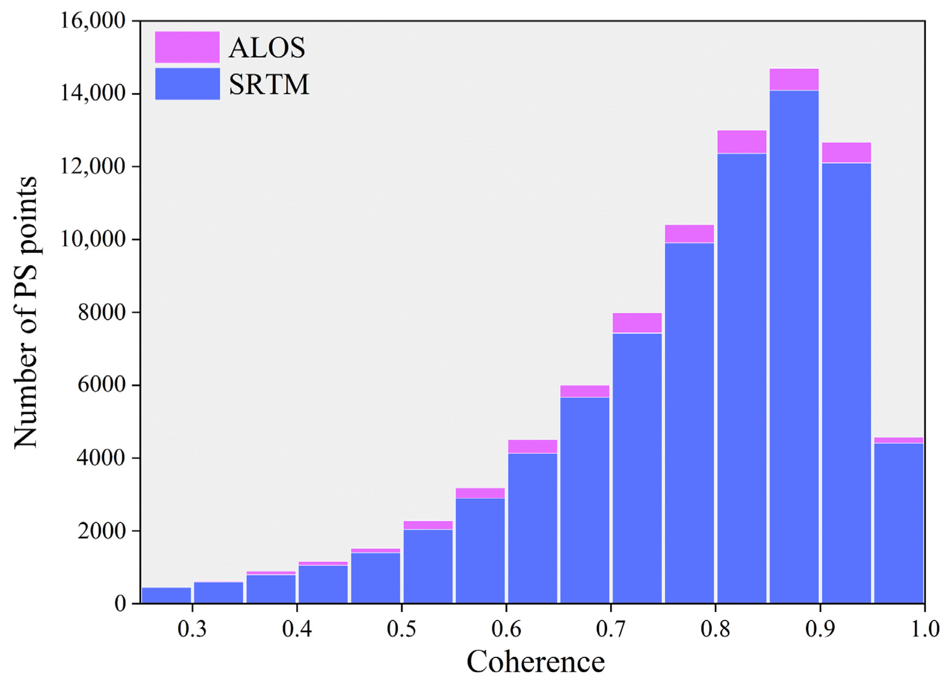
5.2. Effect of Two External DEMs on StaMPS-PS

After co-registration, SAR images were used to remove the terrain phase using an external DEM. Differences in different external DEMs can lead to different terrain residuals in the differential interferogram [47], consequently affecting the initial phase accuracy of StaMPS-PS. Research showed that high-resolution external DEM can improve the density of PS points and enhance the accuracy of estimating the average deformation rate [35]. Therefore, the ALOS PALSAR DEM and SRTM-1 arc DEM were used as external DEMs to study the effects of two DEMs on the monitoring results of StaMPS-PS deformation based on Sentinel-1A images. Because of the difference in resolution between the ALOS PALSAR DEM and the SRTM-1 arc DEM, the latitude and longitude of the selected PS points can also differ, resulting in differences in PS point selection. Overall, there is no significant difference in the spatial distribution of PS points between them. When the ALOS PALSAR DEM was used as the external DEM, 83,819 PS points were selected, whereas when the SRTM-1 arc DEM was used, 83,327 PS points were selected. The number of PS points selected by ALOS was 492, more than that selected by SRTM. Figure 13 shows the number of PS points for the two external DEMs in each coherence interval. When coherence γ > 0.35, the number of PS points with the ALOS PALSAR DEM as the external DEM was greater than that of the SRTM-1 arc DEM, and in the high-coherence region (γ > 0.7), the number of PS points with ALOS was much higher than that of SRTM. The results show that the improvement in the external DEM resolution improves the coherence of the PS points of the StaMPS-PS technology based on the Sentinel-1 image.
Section 4.1 showed deformation monitoring accuracy was higher when ALOS PALSAR DEM was used. To further investigate the relationship between the external DEM and deformation rate, the intersection of the PS points of the two types of DEM was statistically analyzed, and the differences in deformation rate between these common PS points were calculated. The mean differences in deformation rate for these common points were 0.07 mm/year, with a standard deviation of 1.33 mm/year. To analyze the influence of DEM differences on the deformation rate calculation results, the DEM differences were equally divided into eight intervals, and the mean deformation rate values of each interval were calculated and plotted in a histogram. As shown in Figure 14, as the DEM differences increased, the mean deformation rate differences also increased, indicating that the larger the DEM residuals, the greater the impact on the mean deformation rate.

6. Conclusions

Based on the StaMPS-PS method, the monitoring results of Sentinel-1 in Hohhot subway for six years showed that there are three settlement areas in Subway Line 1. The highest subsidence rate reached −17 mm/year. Especially the subsidence trend of the section between Kongjiaying Station and Affiliated Hospital Station conformed to the impacts of subway construction, which is speculated to be related to subway construction. There are three evident subsidence areas in subway line 2, with a settlement rate of −21 mm/year. The subsidence trends in these three areas are consistent with the impact of subway construction. The spatio-temporal analysis of the evident settlement area showed that there are settlement troughs generated by the construction of subway tunnels in the Hugangdonglu section of Line 1 and the Zhongshanlu section of Line 2. The width and maximum subsidence of the settlement troughs gradually expanded during the construction of the subway. The predicted trend using the LSTM model was in good agreement with the real trend, with an RMSE and MAPE of less than 4 mm and 10%, respectively, for typical points, indicating that the LSTM model is feasible for the time-series prediction of the Hohhot subway.
The comparative results of StaMPS-PS using two DEMs showed that the ALOS PALSAR DEM had higher accuracy in this area. Different DEM resolutions impact the number and coherence of the selected PS points. For example, a higher-resolution ALOS PALSAR DEM results in more PS points with higher coherence. Furthermore, an analysis of the difference between the DEMs and deformation rate showed that the difference in the deformation monitoring results increased with an increase in DEM differences. For the Hohhot area, the adoption of high-resolution external DEM can improve the accuracy of StaMPS-PS results and the stability of PS points.

Author Contributions

S.Z. and P.L. performed the experiments and produced the results. H.L. and B.W. performed in data management. T.Z. provided experimental ideas. All authors have read and agreed to the published version of the manuscript.

Funding

This research was funded by the Natural Science Foundation of China (Grant No. 52174160), Fundamental Research Funds for the Central Universities (Grant Nos. 2023YQDC01 and 2023YJSDC08), and the Ecological-Smart Mines Joint Research Fund of the Natural Science Foundation of Hebei Province (Grant No. E2020402086) and open funds from the State Key Laboratory of Coal Mining and Clean Utilization (Granted No. 2021-CMCU-KF014).

Data Availability Statement

Not applicable.

Acknowledgments

The authors would like to acknowledge the open datasets of Sentinel-1 and ALOS PALSAR DEM, and the data processing soft SNAP provided by the European Space Agency (ESA).

Conflicts of Interest

The authors declare no conflict of interest.

References

  1. Chen, F.; Lin, H.; Zhang, Y.; Lu, Z. Ground Subsidence Geo-Hazards Induced by Rapid Urbanization: Implications from InSAR Observation and Geological Analysis. Nat. Hazards Earth Syst. Sci. 2012, 12, 935–942. [Google Scholar] [CrossRef] [Green Version]
  2. Qiu, J.; Qin, Y.; Feng, Z.; Wang, L.; Wang, K. Safety Risks and Protection Measures for City Wall during Construction and Operation of Xi’an Metro. J. Perform. Constr. Facil. 2020, 34, 04020003. [Google Scholar] [CrossRef]
  3. Gupta, S.; Stanus, Y.; Lombaert, G.; Degrande, G. Influence of Tunnel and Soil Parameters on Vibrations from Underground Railways. J. Sound Vib. 2009, 327, 70–91. [Google Scholar] [CrossRef]
  4. Qin, D.; He, P.; Zhang, H.; Ma, C. Analysis on the Safety of a Concrete-Masonry Structure near to Shield Tunnel Excavation. In Proceedings of the 2011 International Conference on Business Management and Electronic Information, Guangzhou, China, 13–15 May 2011; Volume 4, pp. 889–892. [Google Scholar]
  5. Li, X.; Zhang, Y.; Li, Z.; Wang, R. Response of the Groundwater Environment to Rapid Urbanization in Hohhot, the Provincial Capital of Western China. J. Hydrol. 2021, 603, 127033. [Google Scholar] [CrossRef]
  6. Wang, B.; Zhao, C.; Zhang, Q.; Peng, M. Sequential InSAR Time Series Deformation Monitoring of Land Subsidence and Rebound in Xi’an, China. Remote Sens. 2019, 11, 2854. [Google Scholar] [CrossRef] [Green Version]
  7. Mahmutoğlu, Y. Surface Subsidence Induced by Twin Subway Tunnelling in Soft Ground Conditions in Istanbul. Bull. Eng. Geol. Environ. 2011, 70, 115–131. [Google Scholar] [CrossRef]
  8. Qie, Z.; Yan, H. A Causation Analysis of Chinese Subway Construction Accidents Based on Fault Tree Analysis-Bayesian Network. Front. Psychol. 2022, 13, 887073. [Google Scholar] [CrossRef]
  9. Kavvadas, M.J. Monitoring Ground Deformation in Tunnelling: Current Practice in Transportation Tunnels. Eng. Geol. 2005, 79, 93–113. [Google Scholar] [CrossRef]
  10. Wu, J.; Hu, F. Monitoring Ground Subsidence along the Shanghai Maglev Zone Using TerraSAR-X Images. IEEE Geosci. Remote Sens. Lett. 2017, 14, 117–121. [Google Scholar] [CrossRef]
  11. Yan, Y.; Doin, M.-P.; Lopez-Quiroz, P.; Tupin, F.; Fruneau, B.; Pinel, V.; Trouve, E. Mexico City Subsidence Measured by InSAR Time Series: Joint Analysis Using PS and SBAS Approaches. IEEE J. Sel. Top. Appl. Earth Obs. Remote Sens. 2012, 5, 1312–1326. [Google Scholar] [CrossRef] [Green Version]
  12. Liu, J.; Wang, Y.; Li, Y.; Dang, L.; Liu, X.; Zhao, H.; Yan, S. Underground Coal Fires Identification and Monitoring Using Time-Series InSAR with Persistent and Distributed Scatterers: A Case Study of Miquan Coal Fire Zone in Xinjiang, China. IEEE Access 2019, 7, 164492–164506. [Google Scholar] [CrossRef]
  13. Zhao, R.; Li, Z.; Feng, G.; Wang, Q.; Hu, J. Monitoring Surface Deformation over Permafrost with an Improved SBAS-InSAR Algorithm: With Emphasis on Climatic Factors Modeling. Remote Sens. Environ. 2016, 184, 276–287. [Google Scholar] [CrossRef]
  14. Du, Y.; Zhang, L.; Feng, G.; Lu, Z.; Sun, Q. On the Accuracy of Topographic Residuals Retrieved by MTInSAR. IEEE Trans. Geosci. Remote Sens. 2017, 55, 1053–1065. [Google Scholar] [CrossRef]
  15. Talib, O.-C.; Shimon, W.; Sarah, K.; Tonian, R. Detection of Sinkhole Activity in West-Central Florida Using InSAR Time Series Observations. Remote Sens. Environ. 2022, 269, 112793. [Google Scholar] [CrossRef]
  16. Tsironi, V.; Ganas, A.; Karamitros, I.; Efstathiou, E.; Koukouvelas, I.; Sokos, E. Kinematics of Active Landslides in Achaia (Peloponnese, Greece) through InSAR Time Series Analysis and Relation to Rainfall Patterns. Remote Sens. 2022, 14, 844. [Google Scholar] [CrossRef]
  17. Schlögl, M.; Gutjahr, K.; Fuchs, S. The Challenge to Use Multi-Temporal InSAR for Landslide Early Warning. Nat. Hazards 2022, 112, 2913–2919. [Google Scholar] [CrossRef]
  18. Serkhane, A.; Benfedda, A.; Guettouche, M.S.; Bouhadad, Y. InSAR Derived Co-Seismic Deformation Triggered by the Mihoub (Tell Atlas of Algeria) 28 May 2016 (Mw = 5.4) Earthquake Combined to Geomorphic Features Analysis to Identify the Causative Active Fault. J. Afr. Earth Sci. 2022, 188, 104476. [Google Scholar] [CrossRef]
  19. Tong, X.; Xu, X.; Chen, S. Coseismic Slip Model of the 2021 Maduo Earthquake, China from Sentinel-1 InSAR Observation. Remote Sens. 2022, 14, 436. [Google Scholar] [CrossRef]
  20. Li, Y.; Li, Y.; Liang, K.; Li, H.; Jiang, W. Coseismic Displacement and Slip Distribution of the 21 May 2021 Mw 6.1 Earthquake in Yangbi, China Derived from InSAR Observations. Front. Environ. Sci. 2022, 10, 857739. [Google Scholar] [CrossRef]
  21. Liu, Z.; Qiu, H.; Zhu, Y.; Liu, Y.; Yang, D.; Ma, S.; Zhang, J.; Wang, Y.; Wang, L.; Tang, B. Efficient Identification and Monitoring of Landslides by Time-Series InSAR Combining Single- and Multi-Look Phases. Remote Sens. 2022, 14, 1026. [Google Scholar] [CrossRef]
  22. Fernández-Torres, E.A.; Cabral-Cano, E.; Novelo-Casanova, D.A.; Solano-Rojas, D.; Havazli, E.; Salazar-Tlaczani, L. Risk Assessment of Land Subsidence and Associated Faulting in Mexico City Using InSAR. Nat. Hazards 2022, 112, 37–55. [Google Scholar] [CrossRef]
  23. Cigna, F.; Tapete, D. Urban Growth and Land Subsidence: Multi-Decadal Investigation Using Human Settlement Data and Satellite InSAR in Morelia, Mexico. Sci. Total Environ. 2022, 811, 152211. [Google Scholar] [CrossRef] [PubMed]
  24. Luo, Q.; Perissin, D.; Zhang, Y.; Jia, Y. L- and X-Band Multi-Temporal InSAR Analysis of Tianjin Subsidence. Remote Sens. 2014, 6, 7933–7951. [Google Scholar] [CrossRef] [Green Version]
  25. Liu, L.; Gong, H.; Yu, J.; Li, X.; Ke, Y. Stable Pointwise Target Detection Method and Small Baseline Subset INSAR Used in Beijing Subsidence Monitoring. Natl. Remote Sens. Bull. 2016, 20, 643–652. [Google Scholar] [CrossRef]
  26. Luo, X.G.; Wang, J.; Xu, Z.; Zhu, S.; Meng, L.; Liu, J.; Cui, Y. Dynamic Analysis of Urban Ground Subsidence in Beijing Based on the Permanent Scattering InSAR Technology. JARS 2018, 12, 026001. [Google Scholar] [CrossRef]
  27. Ding, C.; Feng, G.; Li, Z.; Shan, X.; Du, Y.; Wang, H. Spatio-Temporal Error Sources Analysis and Accuracy Improvement in Landsat 8 Image Ground Displacement Measurements. Remote Sens. 2016, 8, 937. [Google Scholar] [CrossRef] [Green Version]
  28. Wang, H.; Feng, G.; Xu, B.; Yu, Y.; Li, Z.; Du, Y.; Zhu, J. Deriving Spatio-Temporal Development of Ground Subsidence Due to Subway Construction and Operation in Delta Regions with PS-InSAR Data: A Case Study in Guangzhou, China. Remote Sens. 2017, 9, 1004. [Google Scholar] [CrossRef] [Green Version]
  29. Wang, R.; Yang, M.; Dong, J.; Liao, M. Investigating Deformation along Metro Lines in Coastal Cities Considering Different Structures with InSAR and SBM Analyses. Int. J. Appl. Earth Obs. Geoinf. 2022, 115, 103099. [Google Scholar] [CrossRef]
  30. Yang, M.; Wang, R.; Li, M.; Liao, M. A PSI Targets Characterization Approach to Interpreting Surface Displacement Signals: A Case Study of the Shanghai Metro Tunnels. Remote Sens. Environ. 2022, 280, 113150. [Google Scholar] [CrossRef]
  31. Espiritu, K.W.; Reyes, C.J.; Benitez, T.M.; Tokita, R.C.; Galvez, L.J.; Ramirez, R. Sentinel-1 Interferometric Synthetic Aperture Radar (InSAR) Reveals Continued Ground Deformation in and around Metro Manila, Philippines, Associated with Groundwater Exploitation. Nat. Hazards 2022, 114, 3139–3161. [Google Scholar] [CrossRef]
  32. Bayer, B.; Schmidt, D.; Simoni, A. The Influence of External Digital Elevation Models on PS-InSAR and SBAS Results: Implications for the Analysis of Deformation Signals Caused by Slow Moving Landslides in the Northern Apennines (Italy). IEEE Trans. Geosci. Remote Sens. 2017, 55, 2618–2631. [Google Scholar] [CrossRef]
  33. Ducret, G.; Doin, M.-P.; Grandin, R.; Lasserre, C.; Guillaso, S. DEM Corrections Before Unwrapping in a Small Baseline Strategy for InSAR Time Series Analysis. IEEE Geosci. Remote Sens. Lett. 2014, 11, 696–700. [Google Scholar] [CrossRef]
  34. Torun, A.T.; Ekercin, S.; Algancı, U.; Yılmaztürk, F. Evaluating the Effect of External DEMs on the Accuracy of InSAR DEM Generation. J. Indian Soc. Remote Sens. 2023, 51, 213–225. [Google Scholar] [CrossRef]
  35. Du, Y.; Feng, G.; Li, Z.; Peng, X.; Zhu, J.; Ren, Z. Effects of External Digital Elevation Model Inaccuracy on StaMPS-PS Processing: A Case Study in Shenzhen, China. Remote Sens. 2017, 9, 1115. [Google Scholar] [CrossRef] [Green Version]
  36. Das, A.; Agrawal, R.; Mohan, S. Topographic Correction of ALOS-PALSAR Images Using InSAR-Derived DEM. Geocarto Int. 2015, 30, 145–153. [Google Scholar] [CrossRef]
  37. Liu, M.; Tan, Z.; Fan, X.; Chang, Y.; Wang, L.; Yin, X. Application of Life Cycle Assessment for Municipal Solid Waste Management Options in Hohhot, People’s Republic of China. Waste Manag. Res. 2021, 39, 63–72. [Google Scholar] [CrossRef]
  38. Wang, J.; He, Z. Responses of Stream Geomorphic Indices to Piedmont Fault Activity in the Daqingshan Area of China. J. Earth Sci. 2020, 31, 978–987. [Google Scholar] [CrossRef]
  39. Xu, D.; He, Z.; Ma, B.; Long, J.; Zhang, H.; Liang, K. Vertical Slip Rates of Normal Faults Constrained by Both Fault Walls: A Case Study of the Hetao Fault System in Northern China. Front. Earth Sci. 2022, 10, 816922. [Google Scholar] [CrossRef]
  40. Dong, S.; Liu, B.; Shi, X.; Zhang, W.; Li, Z. The Spatial Distribution and Hydrogeological Controls of Fluoride in the Confined and Unconfined Groundwater of Tuoketuo County, Hohhot, Inner Mongolia, China. Environ. Earth Sci. 2015, 74, 325–335. [Google Scholar] [CrossRef]
  41. Chen, J.; Zhang, Y.; Chen, Z.; Nie, Z. Improving Assessment of Groundwater Sustainability with Analytic Hierarchy Process and Information Entropy Method: A Case Study of the Hohhot Plain, China. Environ. Earth Sci. 2015, 73, 2353–2363. [Google Scholar] [CrossRef]
  42. Chen, C.; Zebker, H. Two-Dimensional Phase Unwrapping with Use of Statistical Models for Cost Functions in Nonlinear Optimization. J. Opt. Soc. Am. A Opt. Image Sci. Vis. 2001, 18, 338–351. [Google Scholar] [CrossRef] [Green Version]
  43. Hooper, A.; Segall, P.; Zebker, H. Persistent Scatterer Interferometric Synthetic Aperture Radar for Crustal Deformation Analysis, with Application to Volcán Alcedo, Galápagos. J. Geophys. Res. Solid Earth 2007, 112, B07407. [Google Scholar] [CrossRef] [Green Version]
  44. Hooper, A.; Zebker, H.; Segall, P.; Kampes, B. A New Method for Measuring Deformation on Volcanoes and Other Natural Terrains Using InSAR Persistent Scatterers. Geophys. Res. Lett. 2004, 31, L23611. [Google Scholar] [CrossRef]
  45. Hooper, A. A Multi-Temporal InSAR Method Incorporating Both Persistent Scatterer and Small Baseline Approaches. Geophys. Res. Lett. 2008, 35, L16302. [Google Scholar] [CrossRef] [Green Version]
  46. Hooper, A.; Zebker, H.A. Phase Unwrapping in Three Dimensions with Application to InSAR Time Series. J. Opt. Soc. Am. A Opt. Image Sci. Vis. 2007, 24, 2737–2747. [Google Scholar] [CrossRef] [Green Version]
  47. Esmaeili, M.; Motagh, M. Psinsar Improvement Using Amplitude Dispersion Index Optimization of Dual Polarimetry Data. ISPRS Int. Arch. Photogramm. Remote Sens. Spat. Inf. Sci. 2015, XL-1-W5, 175–177. [Google Scholar] [CrossRef] [Green Version]
  48. Zebker, H.A.; Villasenor, J. Decorrelation in Interferometric Radar Echoes. IEEE Trans. Geosci. Remote Sens. 1992, 30, 950–959. [Google Scholar] [CrossRef] [Green Version]
  49. Sun, H.X.; Zhao, W.; Yu, J.J. Predication and Analysis on Ground Settlement Induced by Shielding Tunneling Construction. AMR 2011, 261–263, 1156–1160. [Google Scholar] [CrossRef]
  50. Peng, M.; Zhao, C.; Zhang, Q.; Lu, Z.; Bai, L.; Bai, W. Multi-Scale and Multi-Dimensional Time Series InSAR Characterizing of Surface Deformation over Shandong Peninsula, China. Appl. Sci. 2020, 10, 2294. [Google Scholar] [CrossRef] [Green Version]
  51. Ma, L.; Ding, L.; Luo, H. Non-Linear Description of Ground Settlement over Twin Tunnels in Soil. Tunn. Undergr. Space Technol. 2014, 42, 144–151. [Google Scholar] [CrossRef]
  52. Xu, B.; Feng, G.; Li, Z.; Wang, Q.; Wang, C.; Xie, R. Coastal Subsidence Monitoring Associated with Land Reclamation Using the Point Target Based SBAS-InSAR Method: A Case Study of Shenzhen, China. Remote Sens. 2016, 8, 652. [Google Scholar] [CrossRef] [Green Version]
  53. Zhang, Q.; Wang, H.; Dong, J.; Zhong, G.; Sun, X. Prediction of Sea Surface Temperature Using Long Short-Term Memory. IEEE Geosci. Remote Sens. Lett. 2017, 14, 1745–1749. [Google Scholar] [CrossRef] [Green Version]
  54. Wu, L.; Wang, L.; Zhang, P.; Li, T.; Yan, Y. Space-Time Residual LSTM Architechture for Distant Speech Recognition. In Proceedings of the 2018 11th International Symposium on Chinese Spoken Language Processing (ISCSLP), Taipei, Taiwan, 26–29 November 2018; pp. 379–383. [Google Scholar]
  55. Xiang, Z.; Yan, J.; Demir, I. A Rainfall-Runoff Model with LSTM-Based Sequence-to-Sequence Learning. Water Resour. Res. 2020, 56, e2019WR025326. [Google Scholar] [CrossRef]
  56. Guo, H.; Yuan, Y.; Wang, J.; Cui, J.; Zhang, D.; Zhang, R.; Cao, Q.; Li, J.; Dai, W.; Bao, H.; et al. Large-Scale Land Subsidence Monitoring and Prediction Based on SBAS-InSAR Technology with Time-Series Sentinel-1A Satellite Data. Remote Sens. 2023, 15, 2843. [Google Scholar] [CrossRef]
  57. Yu, Y.; Si, X.; Hu, C.; Zhang, J. A Review of Recurrent Neural Networks: LSTM Cells and Network Architectures. Neural Comput. 2019, 31, 1235–1270. [Google Scholar] [CrossRef]
  58. Ma, S.; Qiu, H.; Yang, D.; Wang, J.; Zhu, Y.; Tang, B.; Sun, K.; Cao, M. Surface Multi-Hazard Effect of Underground Coal Mining. Landslides 2023, 20, 39–52. [Google Scholar] [CrossRef]
  59. Wang, L.; Qiu, H.; Zhou, W.; Zhu, Y.; Liu, Z.; Ma, S.; Yang, D.; Tang, B. The Post-Failure Spatiotemporal Deformation of Certain Translational Landslides May Follow the Pre-Failure Pattern. Remote Sens. 2022, 14, 2333. [Google Scholar] [CrossRef]
Figure 1. SAR image coverage and study area range: (a) Study area and SAR image coverage; (b) Enlarged study area and metro line distribution map.
Remotesensing 15 04011 g001
Figure 2. Long short-term memory model (LSTM) structure diagram: (a) LSTM neuronal structure; (b) structure of the subsidence prediction model.
Remotesensing 15 04011 g002
Figure 3. Comparison of level results with StaMPS-PS results.
Remotesensing 15 04011 g003
Figure 4. StaMPS-PS results using DEM with 12.5 m ALOS PALSAR DEM.
Remotesensing 15 04011 g004
Figure 5. Deformation profile of subway line 1.
Remotesensing 15 04011 g005
Figure 6. Subway line 1 subsidence area map and statistical histogram of deformation rate distribution: (a) Subsidence area of subway line 1; (b) subsidence area A; (c) subsidence area B; (d) subsidence area C; (e) profile line of Hugangdonglu.
Remotesensing 15 04011 g006
Figure 7. Statistical histogram of deformation rate distribution: (a) Statistical histogram of deformation rate distribution in subsidence area A of subway line 1; (b) statistical histogram of deformation rate distribution in subsidence area B of subway line 1; (c) statistical histogram of deformation rate distribution in subsidence area C of subway line 1. (d) Statistical histogram of deformation rate distribution in subsidence area A of subway line 2; (e) statistical histogram of deformation rate distribution in subsidence area B of subway line 2; (f) statistical histogram of deformation rate distribution in subsidence area C of subway line 2.
Remotesensing 15 04011 g007
Figure 8. Typical PS points of subsidence trend in the subsidence area: (a) Typical PS point subsidence trend in subsidence area A of subway line 1; (b) Typical PS point subsidence trend in subsidence area B of subway line 1; (c) Typical PS point subsidence trend in subsidence area C of subway line 1; (d) Typical PS point subsidence trend in subsidence area A of subway line 2; (e) Typical PS point subsidence trend in subsidence area B of subway line 2; (f) Typical PS point subsidence trend in subsidence area C of subway line 2.
Remotesensing 15 04011 g008
Figure 9. Deformation profile of subway line 2.
Remotesensing 15 04011 g009
Figure 10. Subway line 2 subsidence area map and statistical histogram of deformation rate distribution: (a) Subsidence area of subway line 1; (b) subsidence area A; (c) subsidence area B; (d) subsidence area C; (e) profile line of Zhongshanlu.
Remotesensing 15 04011 g010
Figure 11. Peck formula: (a) Fitting results of the Peck formula for the settlement trough near Hugangdonglu; (b) fitting results of the Peck formula for the settlement trough near Zhongshanlu.
Remotesensing 15 04011 g011
Figure 12. Loss function and prediction chart: (a) Loss function chart of affiliated hospitals; (b) loss function chart of Hugangdonglu; (c) prediction chart of affiliated hospitals; (d) prediction chart of Hugangdonglu.
Remotesensing 15 04011 g012
Figure 13. Statistical chart of coherence under two external DEMs.
Remotesensing 15 04011 g013
Figure 14. Relationship between DEM differences and average deformation rate differences.
Remotesensing 15 04011 g014
Table 1. Sentinel-1 data information. Perp_B (m) denotes the Perpendicular Baseline (m), and Temp_B (day) represents the Temporal Baseline (days).
NoReference ImageSecondary ImagePerp_B
(m)
Temp_B
(Days)
NoReference ImageSecondary ImagePerp_B
(m)
Temp_B
(Days)
12018.06.182015.07.1675.22−1068432018.06.182018.08.29−40.2772
22018.06.182015.08.09−73.44−1044442018.06.182018.09.2218.9996
32018.06.182015.09.02−5.11−1020452018.06.182018.10.16−103.51120
42018.06.182015.09.2624.28−996462018.06.182018.11.0992.64144
52018.06.182015.10.20−55.77−972472018.06.182018.12.0346.35168
62018.06.182015.11.1361.74−948482018.06.182018.12.27−42.91192
72018.06.182015.12.0711.16−924492018.06.182019.01.2051.08216
82018.06.182015.12.31−37.09−900502018.06.182019.02.13−14.76240
92018.06.182016.02.17−14.09−852512018.06.182019.03.09−37.40264
102018.06.182016.03.12−16.58−828522018.06.182019.04.02−23.01288
112018.06.182016.04.05−10.00−804532018.06.182019.04.26−135.11312
122018.06.182016.04.29−36.87−780542018.06.182019.05.2032.02336
132018.06.182016.05.2347.17−756552018.06.182019.06.1351.09360
142018.06.182016.10.0246.62−624562018.06.182019.07.071.10384
152018.06.182016.10.26−23.25−600572018.06.182019.07.3148.62408
162018.06.182016.11.19−57.42−576582018.06.182019.08.24−115.89432
172018.06.182016.12.1394.01−552592018.06.182019.09.176.33456
182018.06.182017.01.0623.64−528602018.06.182019.10.1151.58480
192018.06.182017.01.30−5.35−504612018.06.182019.11.04−64.72504
202018.06.182017.02.2337.50−480622018.06.182019.11.2859.01528
212018.06.182017.03.19−36,91−456632018.06.182019.12.2251.29552
222018.06.182017.04.12−31.74−432642018.06.182020.01.15−12.63576
232018.06.182017.05.06−108.20−408652018.06.182020.02.0860.78600
242018.06.182017.05.30−25.93−384662018.06.182020.03.15−76.36636
252018.06.182017.06.2331.09−360672018.06.182020.04.0859.22660
262018.06.182017.07.17−45.08−336682018.06.182020.05.02−45.93684
272018.06.182017.08.1017.95−312692018.06.182020.07.25−38.84768
282018.06.182017.09.0312.96−288702018.06.182020.08.1827.81792
292018.06.182017.09.27−81.84−264712018.06.182020.09.11−112.47816
302018.06.182017.10.2141.75−240722018.06.182020.10.05−34.57840
312018.06.182017.11.1458.51−216732018.06.182020.10.2947.23864
322018.06.182017.12.0844.06−192742018.06.182020.11.22−42.23888
332018.06.182018.01.01159.21−168752018.06.182020.12.1631.85912
342018.06.182018.01.25−19.82−144762018.06.182021.01.0982.91936
352018.06.182018.02.182.79−120772018.06.182021.02.02−29.08960
362018.06.182018.03.1437.47−96782018.06.182021.02.2641.30984
372018.06.182018.04.071.15−72792018.06.182021.03.22−12.941008
382018.06.182018.05.0163.16−48802018.06.182021.04.15−18.371032
392018.06.182018.05.25−81.31−24812018.06.182021.05.21−44.711068
402018.06.182018.06.1800822018.06.182021.08.1345.031152
412018.06.182018.07.1273.0124832018.06.182021.09.068.841176
422018.06.182018.08.05−18.3048842018.06.182021.09.30−87.071200
852018.06.182021.10.24−21.891224
Table 2. DEM data information.
DEMSpatial Resolution (m)SourceDate of AcquisitionDistribution Range
ALOS PALSAR DEM12.5https://vertex.daac.asf.alaska.edu, accessed on accessed on 20 October 20222000.02.11–2000.02.2160°S–60°N
SRTM-1 arc DEM30http://earthexplorer.usgs.gov/, accessed on accessed on 22 October 20222008.12.22–2009.01.2057°S–60°N
Table 3. Peck formula fitting parameters for settlement trough of Hogangdonglu.
DateR2RMSESmax (mm)i (m)
2016.10.020.93380.3039−4.823.8
2017.04.120.99140.1428−6.030.7
2018.01.010.98130.4643−11.039.4
2018.03.140.91910.9634−13.548.7
Table 4. Peck formula fitting parameters for the settlement trough of Zhongshanlu.
DateR2RMSESmax (mm)i (m)
2016.10.020.91020.4761−5.958
2016.10.260.84970.6767−6.367
2016.12.130.94990.4887−7.852
2017.05.300.95270.4794−7.951
2017.12.080.98160.3826−10.149
Table 5. LSTM model parameters of monitoring points.
RegionModel ParametersParameter Settings
affiliated hospitalInput_size13
Output_size1
Hidden layers2
Hidden layer neurons50
Epoches200
LossMSE
OptimizerAdam
Batch_size16
Dropout0.2
Learning_rate0.01
HugangdongluInput_size12
Output_size1
Hidden layers2
hidden layer neurons50
Epoches200
LossMSE
OptimizerAdam
Batch_size32
Dropout0.2
Learning_rate0.01
Disclaimer/Publisher’s Note: The statements, opinions and data contained in all publications are solely those of the individual author(s) and contributor(s) and not of MDPI and/or the editor(s). MDPI and/or the editor(s) disclaim responsibility for any injury to people or property resulting from any ideas, methods, instructions or products referred to in the content.

