Self-Adaptive Filtering for Ultra-Large-Scale Airborne LiDAR Data in Urban Environments Based on Object Primitive Global Energy Minimization

Abstract

Filtering from airborne LiDAR datasets in urban area is one important process during the building of digital and smart cities. However, the existing filters encounter poor filtering performance and heavy computational burden when processing large-scale and complicated urban environments. To tackle this issue, a self-adaptive filtering method based on object primitive global energy minimization is proposed in this paper. In this paper, mode points were first acquired for generating the mode graph. The mode points were the cluster centers of the LiDAR data obtained in a mean shift algorithm. The graph constructed with mode points was named “mode graph” in this paper. By defining the energy function based on the mode graph, the filtering process is transformed to iterative global energy minimization. In each iteration, the graph cuts technique was adopted to achieve global energy minimization. Meanwhile, the probability of each point belonging to the ground was updated, which would lead to a new refined ground surface using the points whose probabilities were greater than 0.5. This process was iterated until two successive fitted ground surfaces were determined to be close enough. Four urban samples with different urban environments were adopted for verifying the effectiveness of the filter developed in this paper. Experimental results indicate that the developed filter obtained the best filtering performance. Both the total error and the Kappa coefficient are superior to those of the other three classical filtering methods.

1. Introduction

LiDAR technology has been developing rapidly during the previous decades, and it presently can achieve high efficiency and measuring accuracy in obtaining three-dimensional (3D) information. Nowadays, LiDAR technique is employed in many urban applications, including road detection [1], building extraction [2], digital city construction [3,4], etc. For all these applications, point cloud filtering is one key step, since it is of great significance for the subsequent classification or extraction of the ground object elements [3,5].

Filtering methods can be classified into three groups according to the different theories, including slope-based, morphology-based and surface-based approaches [6]. Vosselman [7] first presented the slope-based filter. This method realized filtering based on elevation differences among points. The ground points were distinguished from non-ground points based on the calculated slope of successive points. Meng et al. [8] proposed a multi-direction filter using the similar slope-based strategy. A two-dimensional neighborhood was incorporated to decrease the errors caused by directions. The experimental results showed that this method possesses robustness towards the slope threshold. Susaki [9] improved the slope-based filter by updating the slope parameter self-adaptively. In this method, the slope parameter can be updated after the estimation of the initial DTM, so as to obtain more local terrain information. Rashidi and Rastiveis [10] proposed a slope and progressive window thresholding method. They adopted elevation difference and directional scanning information to avoid the errors caused by the sensitivity to direction. In this method, the threshold values were calculated automatically according to the topographic features and the dimensions of objects. Although various automatic threshold calculation methods have been developed for the slope-based filtering methods, this kind of method cannot achieve satisfactory filtering performance when encountering abrupt terrains [11].

The morphology-based filter removes non-ground points by morphological operations. Zhang et al. [12] developed a famous progressive morphological filter in which filtering windows were changing size gradually. However, the assumption of constant terrain slope in this method might lead to larger filtering errors [13]. To solve this problem, Pingel et al. [14] improved the morphological filter by combining it with the strength of image inpainting method. Experimental results showed that this improved filter can preserve terrain well and maintain a lower type I error. Hui et al. [15] further improved the morphological filter by combining it with the advantages of surface-based filter. In so doing, the robustness of this filter towards steep terrains was enhanced. Although the calculation process and theory of the morphology-based filter is simple and straightforward, this kind of method needs to determine the maximum filtering window size, which affects the filtering accuracy greatly.

One famous surface-based filtering method is the progressive TIN densification (PTD) filtering method, which was first proposed by Axelsson [16]. In this method, a sparse TIN was created and densified iteratively. Zhang and Lin [17] improved the PTD using a smoothness constraint segmentation. After the initial ground seed points are obtained, the smooth constraint segmentation strategy is adopted to expand the ground seed set, so that more ground seeds can be used to generate a fine terrain model. Liu et al. [18] improved the PTD by combining it with the strength of the morphological filter. Different from other PTD methods, this method first applied the morphological filter to obtain ground seeds. In addition to the PTD methods, some researchers applied interpolated surfaces for filtering. Mongus & Žalik [19] proposed a thin-plate-spline interpolated filter with no parameter setting. In each iteration, a coarse surface was interpolated to calculate the residual of each point. The final DTM was obtained by automatic thresholding. Chen et al. [20] extracted ground points with a multiresolution hierarchical classification algorithm. They used the thin-plate-spline method to fit the terrain surface and detected the ground points based on the point residuals from the surface. Cheng et al. [21] adopted a similar strategy to obtain the distance residuals of points from the interpolated surface. Different from other methods, this method applied the skewness balancing principle for filtering non-ground points. In general, the surface-based filters usually perform better than other kinds of methods due to their progressive filtering strategy. However, this kind of method often fails to detect the discontinuities of terrains. Moreover, when encountering huge amounts of points, the surface-based methods will be under enormous computational burdens.

To solve the above difficulties and challenges, this paper developed a filter based on object primitive global energy minimization. The main contributions of this paper can be summarized as follows:

i)

Point clouds filtering is transformed as global energy minimization, which can be solved using graph cuts automatically.

ii)

A mode graph is constructed using the mode points instead of raw LiDAR points, which will reduce the computation load and speed up the implementation efficiency of the method.

iii)

Filtering thresholds can be calculated self-adaptively according to the constantly updated coarse ground surface, so as to protect terrain details and obtain higher filtering accuracy.

The remainder of this paper is organized as follows. In Section 2, the principle of the proposed filter is demonstrated. Section 3 describes experiments conducted and analysis performed using the samples with different terrain features for accessing the applicability and accuracy of the proposed theory. Section 4 contains a discussion on the parameters involved in this method. Section 5 draws conclusions relevant to the proposed filtering method based on the global energy minimization.

2. Methodology

Figure 1 depicts the main steps of the filter developed in this paper. The raw point clouds were first segmented into object primitives using the mean shift segmentation algorithm [22]. In this algorithm, the cluster center was updated by moving it along the mean shift vector until the cluster center was converged to a local maximum of the density function. Subsequently, the final obtained cluster center was named as the mode point. To alleviate computational burden and improve efficiency, these mode points were used for generating the graph, instead of using raw points. By setting a maximum filtering window, ground seeds can be obtained to build a coarse-fitted surface. Subsequently, the initial probability of each point belonging to the ground and the energy function can be calculated. By using the graph cuts technique [23], the energy minimization can be achieved, which will lead to a labeling result. This algorithm works by modeling the problem as a graph in which the data is represented as a weighted graph, and the task is to partition the graph into two disjoint sets (also called cuts) in a way that minimizes the total weight of the cut edges. Then, the probability of each point belonging to ground will be updated, which will lead to a new, refined ground surface using the points whose probabilities are greater than 0.5. Following this, the probability and energy functions of the new iteration can be calculated. This process is iterated until two successive fitted ground surfaces are close enough. To sum up, three main steps are included, namely: Section 2.1, Mode Graph Construction; Section 2.2, Global Energy Minimization; and Section 2.3, Self-adaptive Progressive Filtering.

2.1. Mode Graph Construction

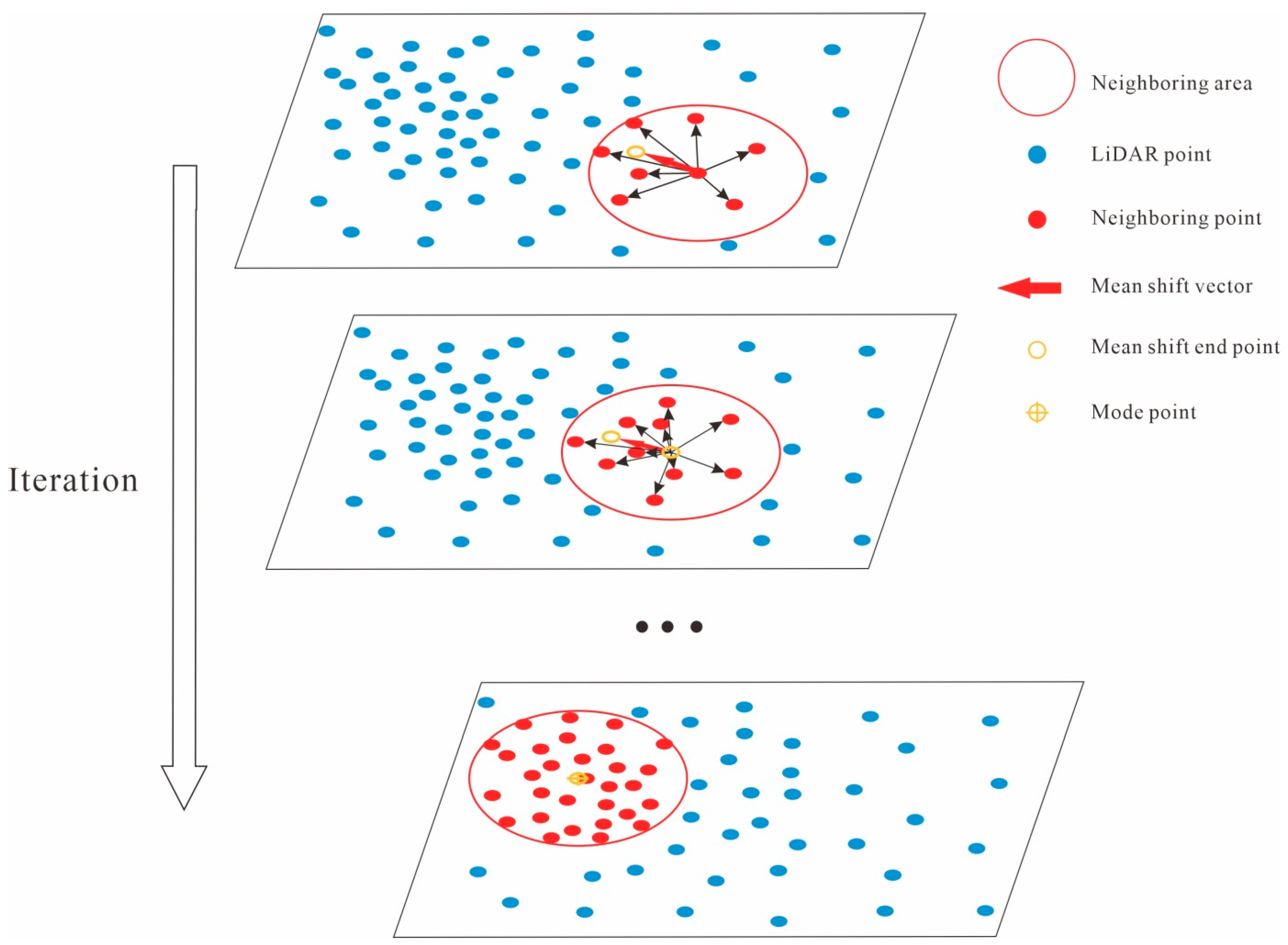
To alleviate the computational burden and create the filtering method applied in large LiDAR datasets, this paper first segmented the point clouds into object primitives. In this paper, a mean shift algorithm was adopted, due to its non-parameter clustering characteristic. Figure 2 shows the segmented process by mean shift method. In each iteration, a mean shift vector defined as the following equation should be calculated.

$$MS\left(C{r}_p\right)={\displaystyle \sum _{i=1}^{n}C{r}_i·Gaussian\left({\Vert \frac{C{r}_p-C{r}_i}{h}\Vert }^2\right)}/{\displaystyle \sum _{i=1}^{n}Gaussian\left({\Vert \frac{C{r}_p-C{r}_i}{h}\Vert }^2\right)}-C{r}_p$$

(1)

where $C{r}_p$ is the coordinate of the central point, $C{r}_i$ is the coordinate of the i-th point in the searching range, and $h$ is the bandwidth. Figure 2 indicates that the mean shift vector points to the direction in which the probability density increases. The mean shift vector will be kept moving until a local maximum is achieved. The local maximum is defined as the mode point.

In this paper, each object primitive is represented by its corresponding mode point. In so doing, huge amounts of LiDAR points can be limited as a series of mode points. Obviously, the computational burden will be relived greatly, especially during the following graph construction.

As mentioned above, instead of raw point clouds, mode points are used for the graph structure building. This paper defines this graph as a mode graph. Likewise, the mode graph contains two components, namely, nodes ($V$) and edges ($E$). The mode graph is defined as $G=\left(V,E\right)$. $V$ is composed by the mode points, while $E$ is the edge between two mode points, which should be met the following conditions.

$$\{\begin{array}{l}V=\left\{p_i|\Vert p_i-Mod{e}^k\Vert =\min ,p_i\in \left\{ob{j}^k\right\}\right\}\hfill \\ E=\left\{E\left(V_i,V_j\right)|V_j\in \mathbb{N}\left(V_i\right)\&\Vert V_i,V_j\Vert \le \delta \right\}\hfill \end{array}$$

(2)

where $p_i$ is the point within the object primitive $ob{j}^k$; $Mod{e}^k$ is the mode point towards $ob{j}^k$; $\Vert ·\Vert$ is the Euclidian distance; and $\mathbb{N}\left(V_i\right)$ means the neighboring points of $V_i$. In this paper, the neighboring points can be achieved based on the three-dimensional Voronoi neighboring system. To remove the influence of the long edge, this paper constrains that the Euclidian distance between two nodes should be smaller than $\delta$, which is defined as the mean distance value plus one standard deviation of the distances between the two neighboring nodes. The mode graph building process is described in Figure 3. It can be seen that the structure of the mode graph is much simpler than that of the graph composed of the raw LiDAR points, while keeping the topology relationship among different object primitives.

2.2. Global Energy Minimization

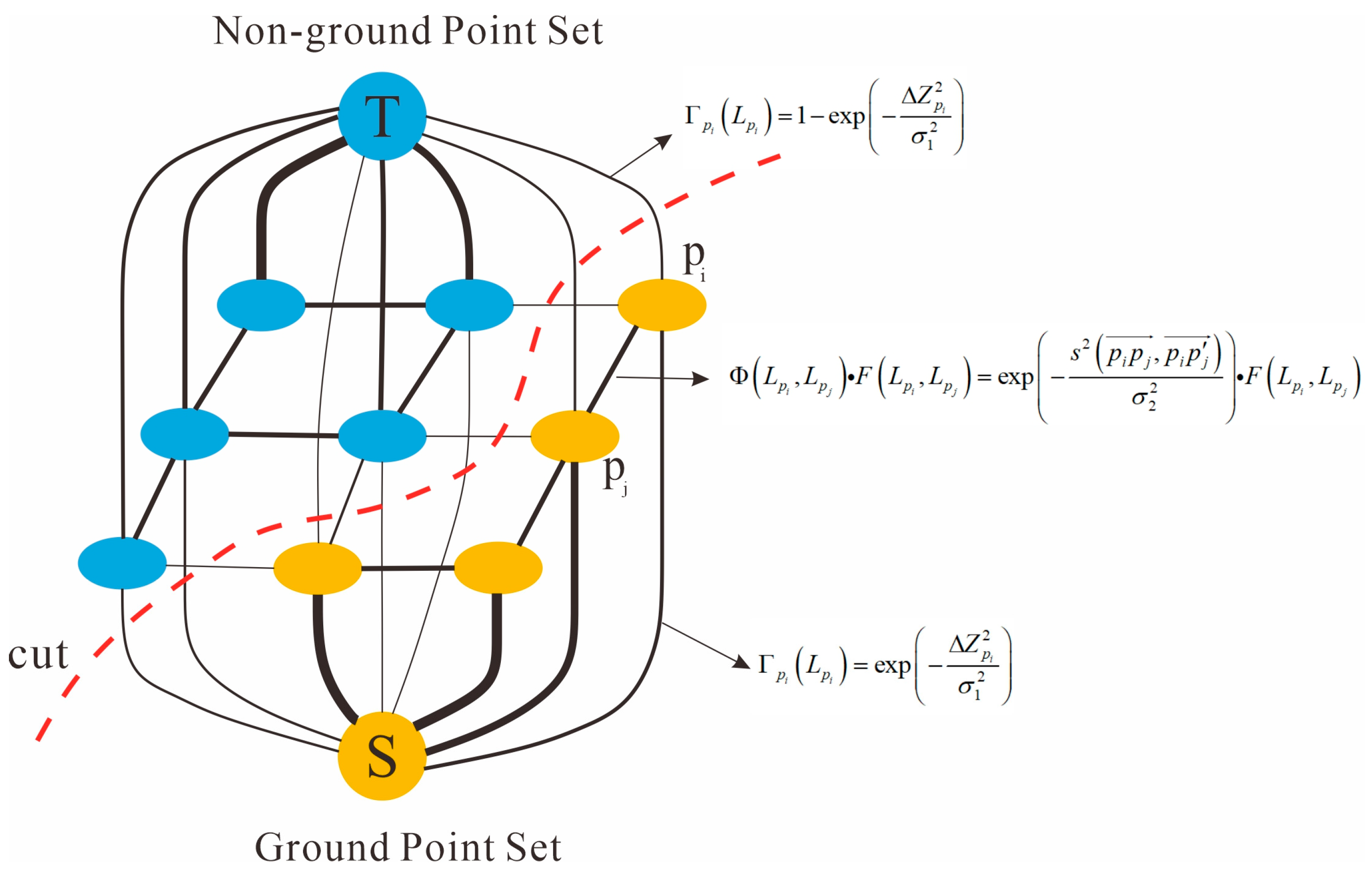
In the mode graph, each node is connected with its neighboring nodes. To realize filtering, these nodes should be separated as two categories, namely, ground point set and non-ground point set. The mode graph is constructed under the assumption that it is connected with two terminal nodes, specifically, source ($S$) and ($T$) sink. In this paper, the highest point in the data is set as T, and the lowest point in the data is set as S. Thus, each node in the graph will be connected to $S$ and $T$, and form link edges. To separate the nodes into ground and non-ground categories, these link edges should be cut to make the nodes connect to only one terminal node. Here, the graph cuts technique [23] was adopted to achieve the separation as illustrated in Figure 4. In this paper, the LiDAR point data was represented as a weighted graph. S and T represented the ground point set and the non-ground point set, respectively. By using the graph cuts algorithm, the point cloud data was divided into two categories.

The minimum graph cuts generally involved energy minimization. The energy function is defined as Equation (3).

$$E\left(L\right)=E_{data}\left(L\right)+\lambda ·E_{smooth}\left(L\right)$$

(3)

where $L$ is a labeling, which will assign the mode point as ground or non-ground label; $\lambda$ is a constant, which balances the contributions of $E_{data}\left(L\right)$ and $E_{smooth}\left(L\right)$ towards $E\left(L\right)$, respectively; and $E_{data}\left(L\right)$ is the data cost, which measures the energy cost when the labeling result is different from the observed data. In this paper, $E_{data}\left(L\right)$ is defined as Equation (4).

$$\{\begin{array}{l}{E}_{data}\left(L\right)={\displaystyle \sum _{i=1}^N{\mathrm{\Gamma }}_{p_i}\left(L_{p_i}\right)}\hfill \\ {\mathrm{\Gamma }}_{p_i}\left(L_{p_i}\right)=\{\begin{array}{c}\exp \left(-\frac{\Delta Z_{p_i}^2}{{\sigma }_1^2}\right),if{C}_{p_i}\ge 0.5\\ 1-\exp \left(-\frac{\Delta Z_{p_i}^2}{{\sigma }_1^2}\right),otherwise\end{array}\hfill \end{array}$$

(4)

where ${\mathrm{\Gamma }}_{p_i}\left(L_{p_i}\right)$ measures the degree of the point $L_{p_i}$ linked to ground and non-ground point sets; ${\sigma }_1$ is a self-adjusted parameter calculated as the mean value of distance residuals of each point to the updated interpolated surface; and $C_{p_i}$ is the probability of a point belonging to ground. In this paper, $C_{p_i}$ is defined as Equation (5).

$$C_{p_i}=\exp \left(-\frac{abs\left(\Delta Z_{p_i}\right)}{{\delta }_1}\right)$$

(5)

where $\Delta Z_{p_i}$ is the distance from $p_i$ to the surface generated by ground seeds based on a radial basis interpolation function and ${\delta }_1$ is a constant parameter, which is set to calculate the probability of each point; the value of ${\delta }_1$ is determined by the experiments described in this paper. From Equation (5), it is easy to find that a larger $\Delta Z_{p_i}$ will lead to a smaller $C_{p_i}$. In other words, it proves that a larger $\Delta Z_{p_i}$ means a smaller probability of the point belonging to the ground. Combined with Equation (4), it establishes that when $C_{p_i}$ is larger than 0.5, a larger $\Delta Z_{p_i}$ will lead to a smaller ${\mathrm{\Gamma }}_{p_i}\left(L_{p_i}\right)$. This indicates that the edge between them is more likely to be cut when minimizing the energy function. Figure 5 shows the data costs for each point at the initial iteration. It can be seen that the ground points tend to be associated with larger ${\mathrm{\Gamma }}_{p_i}\left(L_{p_i}\right)$.

$E_{smooth}\left(L\right)$ is the smooth cost, which evaluates the degree of labeling result that is not piecewise smooth. In this paper, $E_{smooth}\left(L\right)$ is defined as Equation (6).

$$\{\begin{array}{l}{E}_{smooth}\left(L\right)={\displaystyle \sum _{p_j\in \mathbb{N}\left(p_i\right)}\mathrm{\Phi }\left(L_{p_i},L_{p_j}\right)·F\left(L_{p_i},L_{p_j}\right)}\hfill \\ \begin{array}{l}\mathrm{\Phi }\left(L_{p_i},L_{p_j}\right)=\exp \left(-\frac{s^2\left(\overrightarrow{p_i{p}_j},\overrightarrow{p_i{p^{\prime }}_j}\right)}{{\sigma }_2^2}\right)\hfill \\ F\left(L_{p_i},L_{p_j}\right)=\{\begin{array}{l}1,if{C}_{p_i}\ge 0.5\&C_{p_j}<0.5\left|\right|C_{p_i}<0.5\&C_{p_j}\ge 0.5\hfill \\ 0,otherwise\hfill \end{array}\hfill \end{array}\hfill \end{array}$$

(6)

where $\mathrm{\Phi }\left(L_{p_i},L_{p_j}\right)$ measures the disagreement of two neighboring points; ${\sigma }_2$ is a constant parameter, which is set to determine the smooth cost function; $s\left(\overrightarrow{p_i{p}_j},\overrightarrow{p_i{p^{\prime }}_j}\right)$ is the angle between two vectors; $p_j$ is one of the neighboring points of $p_i$; ${p^{\prime }}_j$ is the fitted point of $p_j$ based on the fitted coarse surface; and $F\left(L_{p_i},L_{p_j}\right)$ is an indication function. When $p_i$ and $p_j$ are assigned as different labels, $F\left(L_{p_i},L_{p_j}\right)$ is equal to 1. Otherwise, its value is 0. If the neighboring points are assigned as different labels, that is, $F\left(L_{p_i},L_{p_j}\right)$ is equal to 1, the effective value of $E_{smooth}\left(L\right)$ can be obtained. When $s\left(\overrightarrow{p_i{p}_j},\overrightarrow{p_i{p^{\prime }}_j}\right)$ becomes smaller, the value of $E_{smooth}\left(L\right)$ will become larger. This indicates that the obtained coarse ground surface is closer to the real terrain, and that the surface at this point is smoother. On the contrary, if the obtained coarse ground surface is very different from the real terrain, $s\left(\overrightarrow{p_i{p}_j},\overrightarrow{p_i{p^{\prime }}_j}\right)$ will become larger, and $E_{smooth}\left(L\right)$ will become smaller. Therefore, the $p_i$ in the coarse ground surface can easily be eliminated as a non-ground point during iterations.

2.3. Self-Adaptive Progressive Filtering

As shown in Figure 1, the proposed method is an iterated progressive filtering method. At each iteration, the probability of each point belonging to the ground point set is calculated. Meanwhile, the energy function that includes data costs and smoothness costs is also constructed. After energy minimization using the graph cuts technique, the labeling result of this iteration can be achieved. The detailed steps of the developed filter are tabulated in

Table 1. Steps of progressive filtering.

Input: Mode Points and Mode Graph

Step 1: Achieve initial coarse ground surface $f$.

Step 2: Calculate the distance from each point to the surface ($\Delta Z_{p_i}$).

Step 3: Calculate probability according to Equation (5).

Step 4: Construct energy function using Equations (4) and (6).

Step 5: Energy minimization based on graph cuts as shown in Figure 4.

Step 6: Obtain the labeling results and update the coarse ground surface $f^{’}$.

Step 7: if $ave\left({\displaystyle \sum _{i=1}^{n}abs\left[f\left(x_{p_i},y_{p_i}\right)-f^{’}\left(x_{p_i},y_{p_i}\right)\right]}\right)\le \eta$

obtain the final ground surface as $f^{’}$

break

else

$f=f^{’}$ and go to S2

end

Step 8: Calculate the self-adaptive filtering threshold based on the ground surface.

Output: Filtering Results: $\left\{p_i\in G|\left|Z_{p_i}-Z_{p_i}^{’}\right|\le {\kappa }^2\left(f^{’}\right)+t\right\}$

.

From Table 1, it is easy to see that after each iteration, a coarse ground surface can be acquired. As the iterations proceed, the coarse ground surface progressively changes for the better. The iteration continues until two successive coarse surfaces demonstrate a change smaller than a threshold as defined in Equation (7).

$$\left({\displaystyle \sum _{i=1}^{n}abs\left[f\left(x_{p_i},y_{p_i}\right)-f^{\prime }\left(x_{p_i},y_{p_i}\right)\right]}\right)/n\le \eta$$

(7)

where $f\left(x_{p_1},y_{p_1}\right)$ and $f^{\prime }\left(x_{p_1},y_{p_1}\right)$ represent the fitted elevation values of two successive coarse surfaces; $\eta$ is set to 0.03 m in this paper. This value is achieved through the experiments. A small threshold increases the iterations, which seriously increases the computation cost of the algorithm. On the contrary, a large value for the threshold reduces the authenticity of the final coarse ground surface, which increases the error of the filtering results.

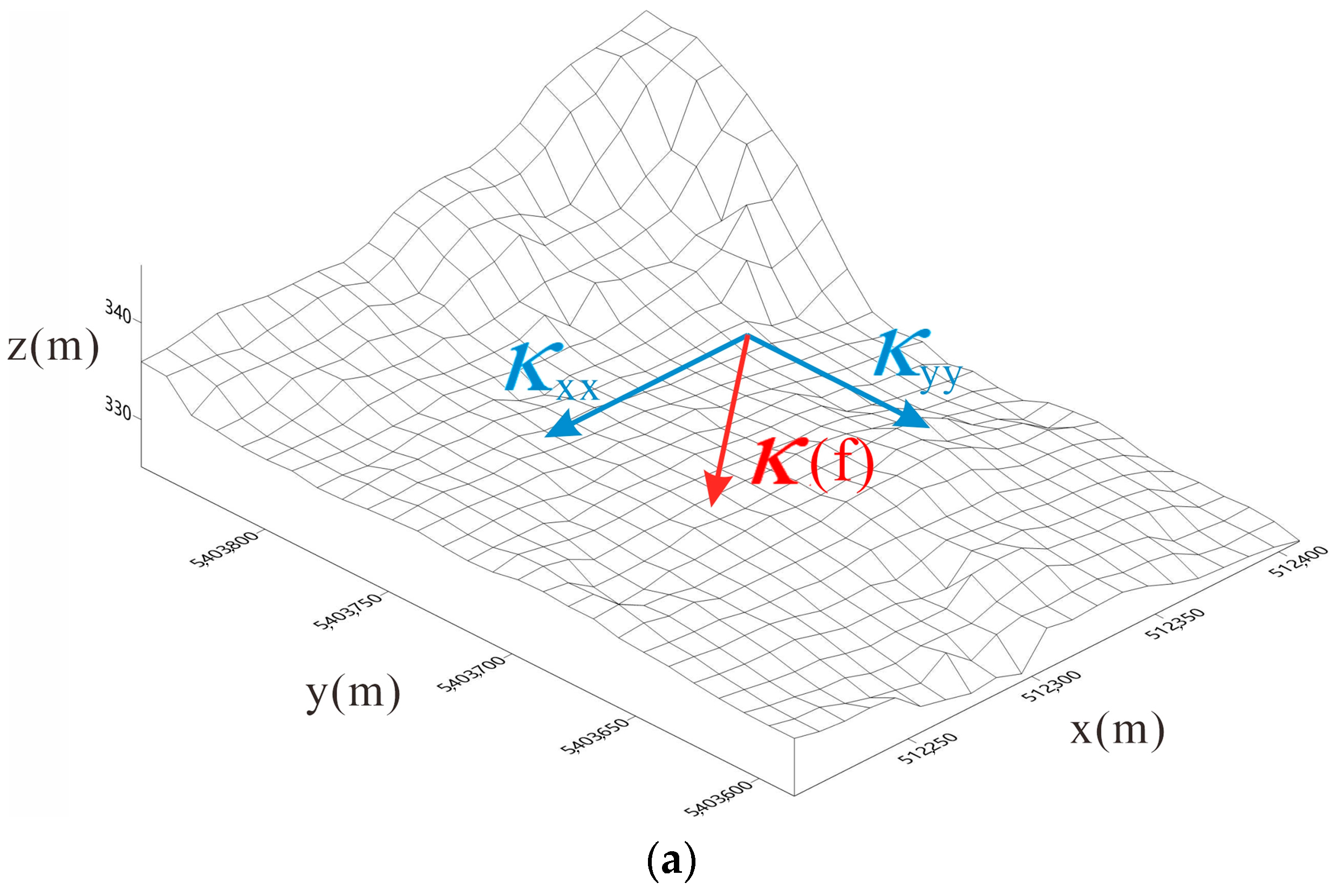
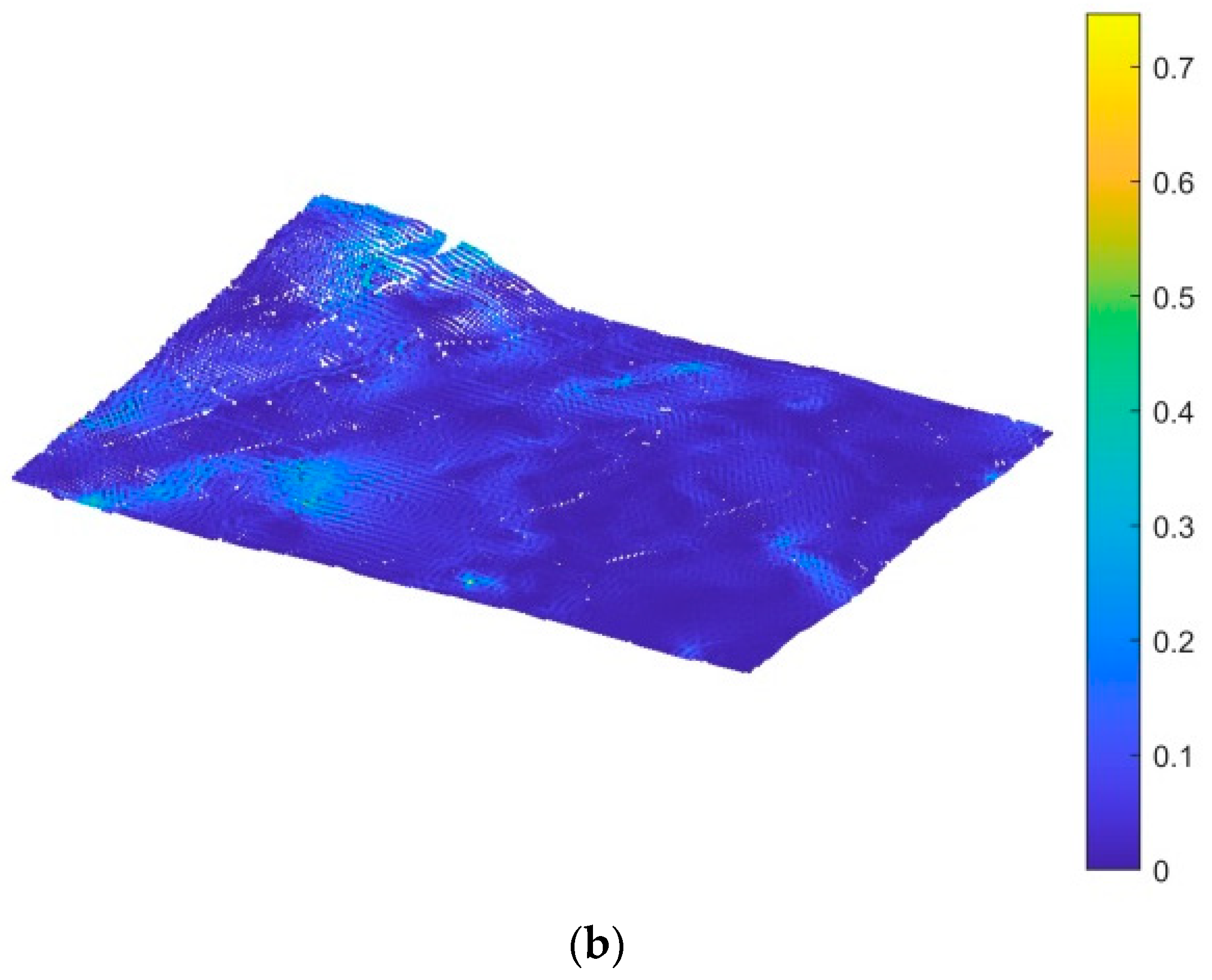
When the final coarse ground surface is achieved, the self-adaptive filtering thresholds can be calculated to realize its values, changing with the relief of the terrain, as shown in Figure 6. The self-adaptive filtering threshold is set according to the slope gradient of the final coarse ground surface, as defined in Equation (8).

$$thr={\kappa }^2\left(f\right)+t$$

(8)

where $\kappa \left(f\right)$ represents the slope gradient and $t$ is a constant. In this paper, $t$ is 0.3 m. This indicates that, when encountering a flat terrain ($\kappa \left(f\right)$ is equal to 0), the points higher than 0.3 m are classified as objects. If the elevation difference between the measured point and the final coarse ground surface is less than the threshold, the point is classified as a terrain point. Otherwise, the point is an object point. This is defined in Equation (9).

$$point=\{\begin{array}{ll}object& \Delta h\ge th{r}_p\\ terrain\_point& \Delta h<th{r}_p\end{array}$$

(9)

where ∆h is the elevation difference between the measured point and the final coarse ground surface and thr_p is the filtering threshold of the point.

3. Experimental Results and Analysis

3.1. Data Description

To evaluate the performance of the proposed method, the public datasets provided by Qin et al. [24] were selected for testing. The datasets contain nine different terrain scenarios and cover a total area of more than 47 km². Among them, S1–S4 are located in urban areas, which is the type used to test the proposed method. As shown in Figure 7, S1 and S2 are relatively flat and contain large buildings and trees. The main objects in S3 and S4 are middle-sized buildings and dense vegetation. The characteristics of the four samples are tabulated in

Table 2. The characteristics of the four tested samples.

Area	Ground Points	Non-Ground Points	Size (m2)	Density (Points/m2)	Objects
S1	1,306,153	1,498,883	500 × 500	11	Large buildings, cars, overpass, low vegetation, trees.
S2	1,783,541	3,690,842	500 × 500	21	Dense buildings, cars, bridges, low vegetation, trees.
S3	137,033	119,707	500 × 500	1	Middle-size buildings, cars, low vegetation, trees.
S4	388,303	375,554	500 × 500	3	Dense middle-size buildings, low vegetation, trees.

. From Table 2, it can be determined that the four samples can test the performance of the proposed method in different urban environments and point densities, so as to verify the effectiveness and robustness of the method. Thus, it can be concluded that the four samples are sufficiently representative for testing filtering methods in ultra-large-scale complex urban areas.

For quantitative evaluation, four indicators were adopted to evaluate the filtering results of the proposed method. They are type I error ($TypeI$), type II error ($Type$ II), total error ($Total$) and kappa coefficient ($Kappa$). Type I error represents the omission error, that is, the percentage of ground points in the reference that were not successfully detected. Type II error is called the commission error, which represents the percentage of the wrongly detected non-ground points compared to the reference. The total error represents the percentage of all misclassified points. The kappa coefficient is another comprehensive indicator used to evaluate the filtering results. The definitions of the above four indicators are defined in Equations (10)–(15):

$$TypeI=\frac{FN}{TP+FN}$$

(10)

$$TypeII=\frac{FP}{FP+TN}$$

(11)

$$Total=\frac{FN+FP}{TP+TN+FN+FP}$$

(12)

$$p_0=\frac{TP+TN}{TP+TN+FP+FN}$$

(13)

$$p_e=\frac{(TP+FP)\ast (TP+FN)+(FP+TN)\ast (FN+TN)}{{(TP+TN+FP+FN)}^2}$$

(14)

$$Kappa=\frac{p_0-p_e}{1-p_e}$$

(15)

where $FN$ is the number of omitted ground points; $FP$ is the number of wrong detected ground points; $TP$ represents the number of correctly detected ground points; and $TN$ is the number of correctly identified non-ground points.

3.2. Experimental Results and Analysis

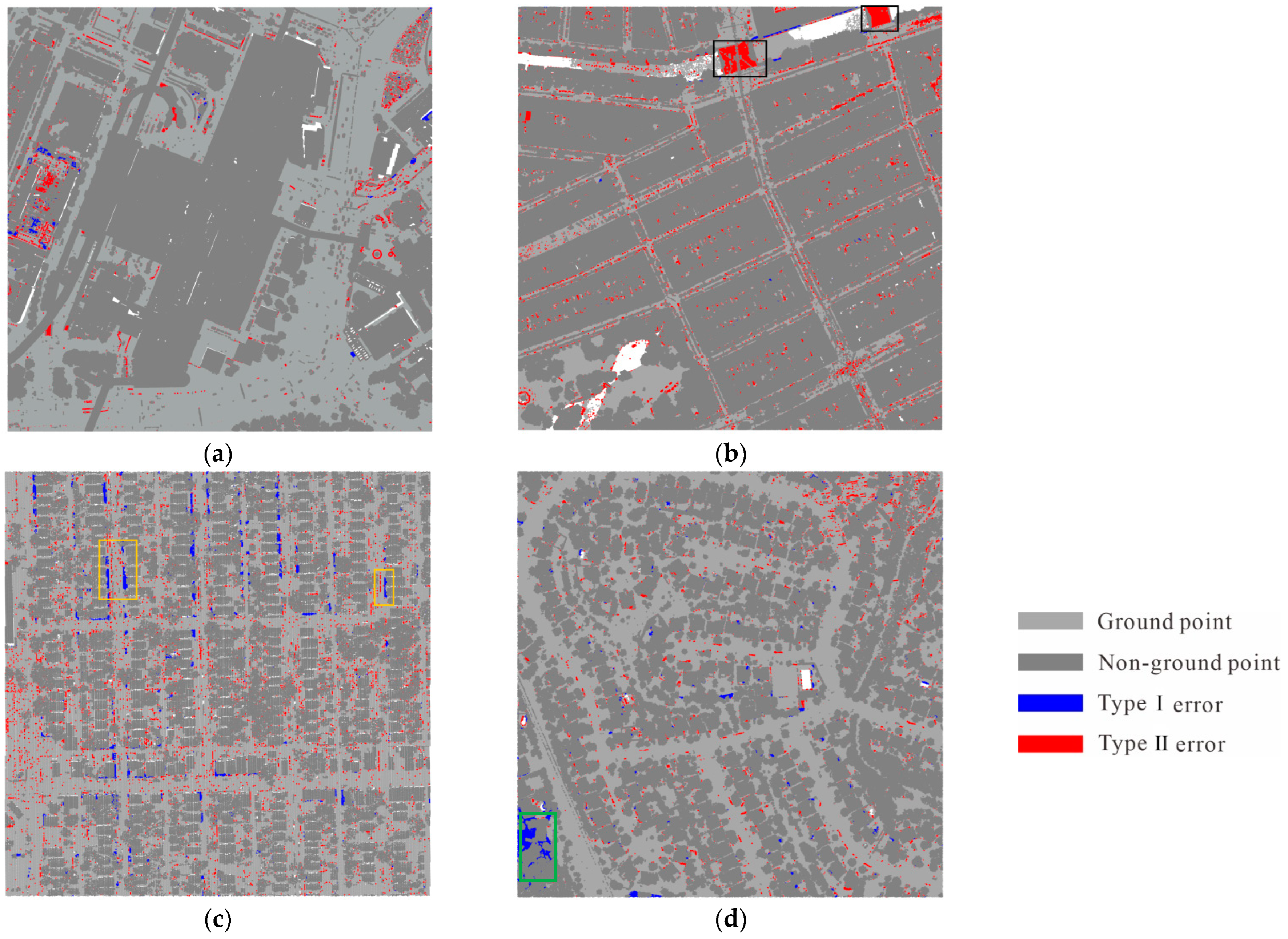
Figure 8 shows the filtering results achieved in the four samples using the proposed method. The light gray represents the correctly detected ground points ($TP$); the dark gray indicates correctly identified non-ground points ($TN$); blue represents the type I error ($TypeI$), that is, the omitted ground points ($FN$); and red represents the type II error ($Type$ II), that is, the wrongly detected ground points. From Figure 8, it can be determined that the proposed method could achieve good filtering results in the four experimental samples. As shown in Figure 8a,b, the proposed method has fewer omitted ground points in S1 and S2. Thus, it can be concluded that the proposed method could effectively eliminate the interference of large buildings in the filtering. However, there are some bridge points that are misclassified as ground in S2, as indicated by the black rectangles shown in Figure 8b. These broad bridges cross the river, and they have insufficient altitude differences with the urban road points. As a result, they are easily misjudged as ground points. In S3, there are some omitted ground points, which are mostly located around middle-sized buildings, as shown in the yellow rectangles of Figure 8c. This is because the point density of S3 is small (1 points/m², according to Table 2), and the elevation values vary greatly between the building points and their adjacent points. Thus, the filtering thresholds calculated according to the local slope are large, so the ground points around the buildings cannot be successfully detected. As shown in the green rectangles of Figure 8d, there are some concentrated omitted ground points in S4. This area is located on the raised terrain, and the small area of exposed ground is surrounded by buildings, resulting in a small elevation difference between ground points and adjacent non-ground points. Therefore, these ground points are easily omitted.

Three classical methods were selected for comparative analysis, namely, progressive morphological filter (PM), cloth simulation filter (CSF) and one surface-based filter developed in the software application named Fusion. The PM filter was presented by Zhang et al. [12]. They increased the window size of the filter step-by-step to remove objects, proceeding from smaller to larger. Zhang et al. [13] proposed the classical CSF method. They assumed that there was a stretchable piece of cloth covering the inverted point cloud data. The ground points are accepted as the locations of cloth nodes. ’The Fusion software [25] belongs to the surface-based filter. In this filter, an average ground surface was calculated, and then weights of points were calculated with the residual. By updating the weights of points, the final ground surface could be achieved.

Table 3. Accuracy comparison of the filtering results in four areas. Bold font represents the best value among the comparison results.

Area	Method	Type I (%)	Type II (%)	Total (%)	$\mathit{K}\mathit{a}\mathit{p}\mathit{p}\mathit{a}$ (%)
S1	PM	13.81	3.87	8.5	82.83
	CSF	3.05	2.34	2.67	94.63
	Fusion	3.4	14.04	9.09	81.89
	The proposed method	0.49	3.19	1.94	96.12
S2	PM	17.56	4.68	8.87	79.38
	CSF	5.65	3.76	4.38	90.09
	Fusion	1.46	4.86	3.75	91.65
	The proposed method	0.67	5.21	3.73	91.72
S3	PM	3.37	8.65	5.83	88.25
	CSF	4.7	7.42	5.97	87.79
	Fusion	3.49	7.55	5.39	89.16
	The proposed method	2	6.92	4.29	91.35
S4	PM	5.01	6.18	5.58	88.82
	CSF	11.04	3.6	7.38	85.25
	Fusion	14.36	2.87	8.71	82.61
	The proposed method	2.08	3.79	2.92	94.15

shows the four accuracy-indicator comparison results. Compared with the other three filters, the developed filter obtained satisfying performances in all four experimental samples. The developed filter obtained the best results on three out of four indicators, specifically, $TypeI$, $Type$ II and $Kappa$. All of the kappa coefficients of the developed filter in the four areas are larger than 90%. It can be concluded that the developed filter can obtain satisfactory filtering performance in different urban samples, and that the method is robust. The type I errors in S1 and S2 areas are less than 1%. This shows that the developed filter can extract more ground points correctly and retain more terrain details. The developed filter achieves the best filtering result in S1. All four indicators in S1 are better than those in the other three samples. In summary, it can be concluded that the developed filter can eliminate the influence of large buildings on the filtering results effectively while detecting the ground points correctly.

Figure 9 shows the comparison of the average accuracy indicators of the developed filter with the three methods, as to the four samples. Among the four average indicators, average $TypeI$, $Type$ II and $Kappa$. of the developed filter are much better than the ones of PM, CSF and Fusion. This indicates that, compared with the other three filters, the developed filter can obtain better filtering performance. As can be seen from Figure 9, the average type II error of the developed filter is a little larger than that of the CSF method. However, the average type I error of the developed filter is significantly smaller than that of the CSF method. Consequently, the total error of the developed filter is the smallest.

To further analyze the filtering effect, this paper selects one profile in sample S4 before and after point clouds filtering using the four different methods, as shown in Figure 10a. Figure 10b shows the raw LiDAR point profile, including both ground and object points. Figure 10c is a real referenced terrain profile. Figure 10d–g, are the filtered terrain profiles by PM, CSF, Fusion and the proposed method, respectively. The developed filter can achieve the closest terrain profile to the referenced terrain profile shown in Figure 10c. All of the other three methods demonstrate an inability to protect terrain details when encountering abrupt terrains, such as the red rectangles shown in Figure 10d–f. In order to further verify the effectiveness of the proposed method, the other profile in sample S4 is selected for comparison, shown as the green line in Figure 10a. Figure 10h shows the raw LiDAR point profile, including dense trees and low buildings. Figure 10i is the real referenced terrain profile. Figure 10j–l and m, are the filtered terrain profiles by PM, CSF, Fusion and the proposed method, respectively. It can be seen that, compared with the proposed method, a large number of ground points are lost in all the other three methods, as evident in the green rectangles shown in Figure 10j–l. The filtering results obtained by the proposed method are very close to the real terrain, as shown in Figure 10i,m.

4. Discussion

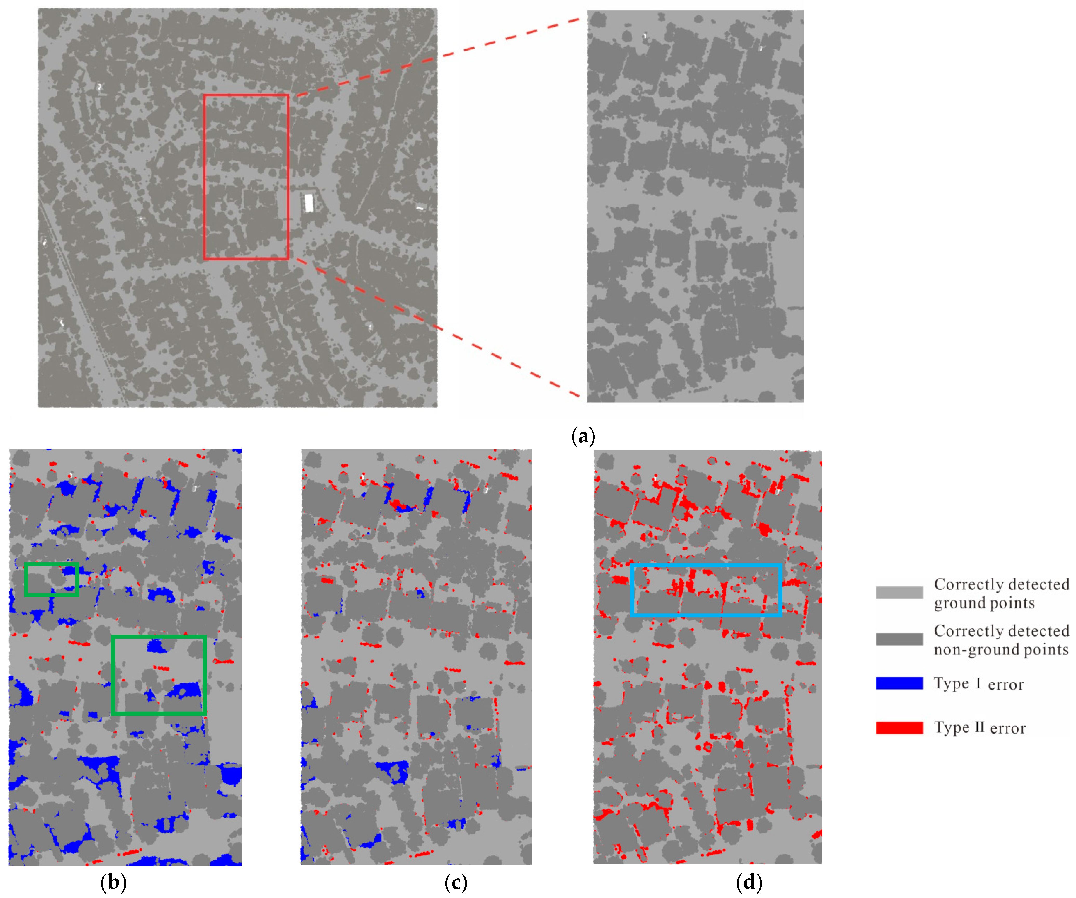
There are three parameters involved during energy minimization, such as ${\sigma }_1$ in Equation (4), ${\delta }_1$ in Equation (5) and ${\sigma }_2$ in Equation (6). Among them, ${\sigma }_1$ was obtained by adaptive calculation based on different experimental data. ${\delta }_1$ and ${\sigma }_2$ were determined based on a large number of experiments. ${\sigma }_1$ was set to determine the data cost function. In this paper, ${\sigma }_1$ can be calculated as the mean value of the distance residuals of each point to the updated interpolated surface in each iteration. Thus, ${\sigma }_1$ can be self-adjusted according to different experimental samples. ${\delta }_1$ was set to calculate the probability of each point belonging to the ground point set. According to Equation (5), it can be determined that the larger ${\delta }_1$ is, the higher the probability is that the points are classified as grounds. This indicates that more points can be classified as grounds in each iteration. On the contrary, when ${\delta }_1$ is set to a smaller value, the calculated probability will be smaller. It means fewer points will be seen as grounds in each iteration. Consequently, more iterations will be needed to achieve final filtering results. Obviously, this will be time-consuming. This paper selected one rectangle area to test the influence of the ${\delta }_1$ setting, as illustrated in Figure 11a. It can be determined that when ${\delta }_1$ is set to 0.5, many ground points are rejected as objects, as seen in the green rectangles shown in Figure 11b. As a result, there is a larger type I error. As a contrast, when ${\delta }_1$ is set to 2, although more ground points are detected, more object points are wrongly accepted as grounds, as seen in the blue rectangle shown in Figure 11d. When ${\delta }_1$ is set to 1, $TypeI$ and $Type$ II errors are balanced, as shown in Figure 11c. This means fewer ground points were rejected while fewer object points were misclassified. Thus, ${\delta }_1$ is set to 1 in this paper.

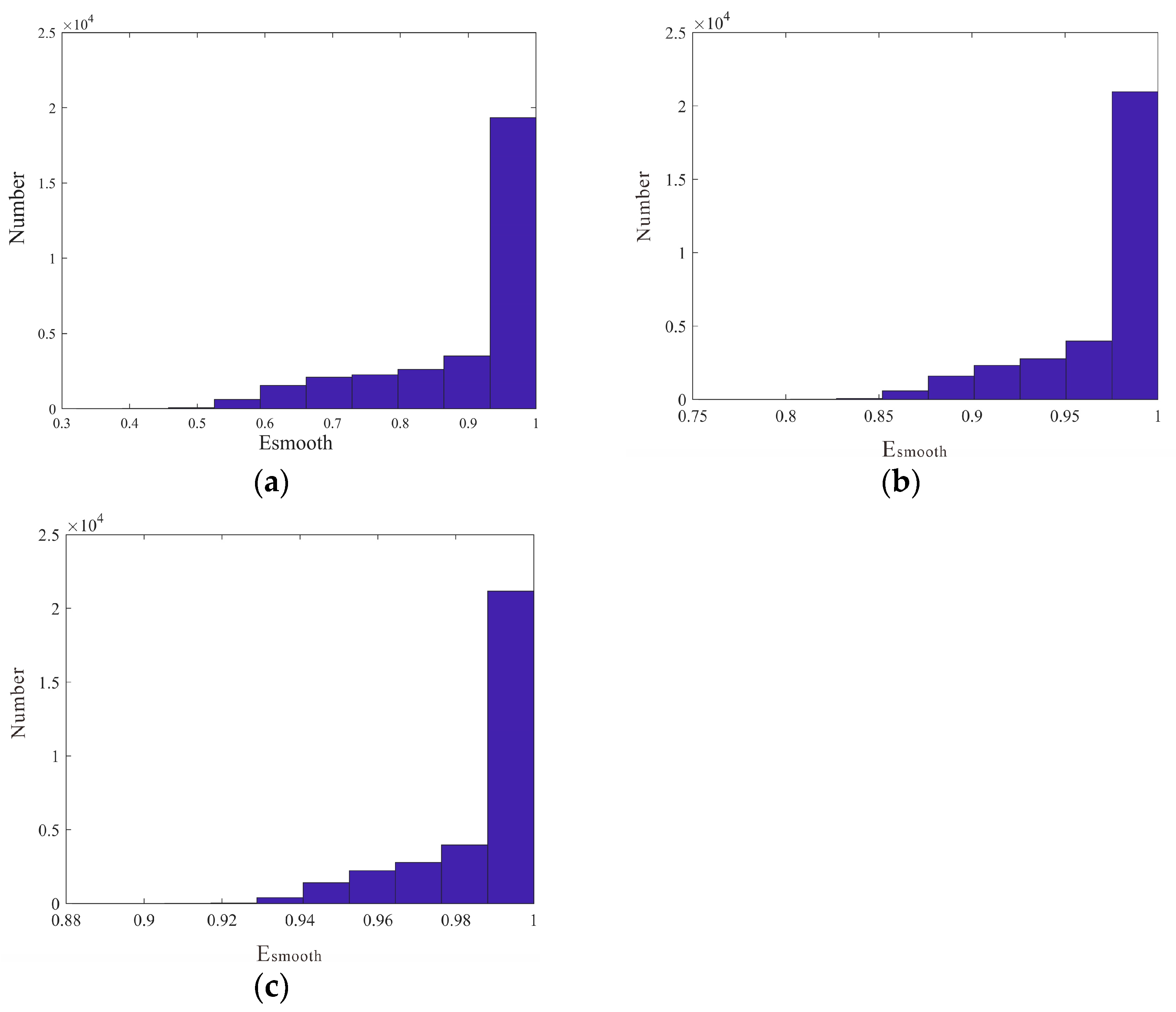
${\sigma }_2$ was set to determine the smooth cost function, as defined in Equation (6). Figure 12 is the distribution histogram of $E_{smooth}$ when ${\sigma }_2$ is set to 2, 4 and 6, respectively. It can be determined that, as the values of ${\sigma }_2$ increase, the distribution of the $E_{smooth}$ becomes more concentrated. This means that the difference of the $E_{smooth}$ for each point becomes smaller. When ${\sigma }_2$ is set to 2, the value range of $E_{smooth}$ is [0.3, 1]. When ${\sigma }_2$ is set to 4, the value range of $E_{smooth}$ is [0.75, 1]. When ${\sigma }_2$ is set to 6, the value range of $E_{smooth}$ is [0.88, 1].

Table 4. Filtering results in S4 with different values of ${\sigma }_2$.

$${\mathit{\sigma }}_2$$	Type I Error (%)	Type II Error (%)	Total Error (%)	Kappa (%)
2	2.59	3.76	3.17	93.67
4	2.08	3.79	2.92	94.15
6	1.60	5.53	3.53	92.93

shows the filtering accuracy in S4 area when ${\sigma }_2$ is set to 2, 4 and 6, respectively. The filtering results show that, with the increasing of ${\sigma }_2$, type I error gradually decreases, while type II error gradually increases. This is because, when ${\sigma }_2$ is set to a larger value, the difference of $E_{smooth}$ among the points is smaller, as shown in Figure 12. As a result, it is easy to accept more points with low elevations as grounds during the energy minimization using the graph cutting technique. However, the smaller difference of $E_{smooth}$ between each point also leads to more low object points being wrongly classified as ground points, which will increase the type II error. Table 4 shows that the total error and kappa coefficient can be optimized when ${\sigma }_2$ is set to 4. In this case, $TypeI$ and $Type$ II errors can be balanced well, and the ideal filtering result can be achieved.

5. Conclusions

Filtering in urban areas is a significant step in building extraction, urban 3D model establishment, digital city construction, etc. To resolve the filtering difficulties, such as heavy computational burden, poor filtering accuracy and robustness, this paper developed a self-adaptive filter based on object primitive global energy minimization. In this paper, point cloud filtering is transformed as global energy minimization. Instead of using all of the points to generate the graph, this paper first applied the mean shift segmentation to obtain mode points. In so doing, the graph built using mode points was made less complicated and the computational burden for graph cuts was greatly reduced. By calculating the global energy and iteratively updating the probability of each point belonging to the ground point set, the final filtering results were achieved. Four public samples were selected for testing. Experimental results showed that the average total error and Kappa coefficient of the developed filter are 3.22% and 93.34%, respectively. These two indices are superior to those of the three classical filtering methods. This reveals that the developed filter can obtain a good filtering effect under different urban environments.

References

1. Jia, J.; Sun, H.; Jiang, C.; Karila, K.; Karjalainen, M.; Ahokas, E.; Khoramshahi, E.; Hu, P.; Chen, C.; Xue, T.; et al. Review on active and passive remote sensing techniques for road extraction. Remote Sens. 2021, 13, 4235. [Google Scholar] [CrossRef]
2. Cai, Z.; Ma, H.; Zhang, L. A building detection method based on semi-suppressed fuzzy c-means and restricted region growing using airborne LiDAR. Remote Sens. 2019, 11, 848. [Google Scholar] [CrossRef] [Green Version]
3. You, H.; Li, S.; Xu, Y.; He, Z.; Wang, D. Tree extraction from airborne laser scanning data in urban areas. Remote Sens. 2021, 13, 3428. [Google Scholar] [CrossRef]
4. Xue, F.; Lu, W.; Chen, Z.; Webster, C.J. From LiDAR point cloud towards digital twin city: Clustering city objects based on gestalt principles. ISPRS J. Photogramm. 2020, 167, 418–431. [Google Scholar] [CrossRef]
5. Zhao, H.; Xi, X.; Wang, C.; Pan, F. Ground surface recognition at voxel scale from mobile laser scanning data in urban environment. IEEE Geosci. Remote Sens. Lett. 2020, 17, 317–321. [Google Scholar] [CrossRef]
6. Cai, S.; Zhang, W.; Liang, X.; Wan, P.; Qi, J.; Yu, S.; Yan, G.; Shao, J. Filtering airborne LiDAR data through complementary cloth simulation and progressive TIN densification filters. Remote Sens. 2019, 11, 1037. [Google Scholar] [CrossRef] [Green Version]
7. Vosselman, G. Slope Based Filtering of Laser Altimetry Data; IAPRS: Amsterdam, The Netherlands, 2000; Volume XXXIII. [Google Scholar]
8. Meng, X.; Wang, L.; Silván-Cárdenas, J.L.; Currit, N. A multi-directional ground filtering algorithm for airborne LIDAR. ISPRS J. Photogramm. 2009, 64, 117–124. [Google Scholar] [CrossRef] [Green Version]
9. Susaki, J. Adaptive slope filtering of airborne LiDAR data in urban areas for digital terrain model (DTM) generation. Remote Sens. 2012, 4, 1804–1819. [Google Scholar] [CrossRef] [Green Version]
10. Rashidi, P.; Rastiveis, H. Extraction of ground points from LiDAR data based on slope and progressive window thresholding (SPWT). Earth Obs. Geomat. Eng. 2018, 2, 36–44. [Google Scholar]
11. Chen, C.; Guo, J.; Wu, H.; Li, Y.; Shi, B. Performance comparison of filtering algorithms for high-density airborne LiDAR point clouds over complex landscapes. Remote Sens. 2021, 13, 2663. [Google Scholar] [CrossRef]
12. Zhang, K.; Chen, S.; Whitman, D.; Shyu, M.; Yan, J.; Zhang, C. A progressive morphological filter for removing nonground measurements from airborne LiDAR data. IEEE Trans. Geosci. Remote Sens. 2003, 41, 872–882. [Google Scholar] [CrossRef] [Green Version]
13. Zhang, W.; Qi, J.; Wan, P.; Wang, H.; Xie, D.; Wang, X.; Yan, G. An easy-to-use airborne LiDAR data filtering method based on cloth simulation. Remote Sens. 2016, 8, 501. [Google Scholar] [CrossRef]
14. Pingel, T.J.; Clarke, K.C.; McBride, W.A. An improved simple morphological filter for the terrain classification of airborne LIDAR data. ISPRS J. Photogramm. 2013, 77, 21–30. [Google Scholar] [CrossRef]
15. Hui, Z.; Hu, Y.; Yevenyo, Y.Z.; Yu, X. An improved morphological algorithm for filtering airborne LiDAR point cloud based on multi-Level kriging interpolation. Remote Sens. 2016, 8, 35. [Google Scholar] [CrossRef] [Green Version]
16. Axelsson, P. DEM generation from laser scanner data using adaptive TIN models. Int. Arch. Photogramm. Remote Sens. 2000, 33, 110–111. [Google Scholar]
17. Zhang, J.; Lin, X. Filtering airborne LiDAR data by embedding smoothness-constrained segmentation in progressive TIN densification. ISPRS J. Photogramm. 2013, 81, 44–59. [Google Scholar] [CrossRef]
18. Liu, X.; Chen, Y.; Cheng, L.; Yao, M.; Deng, S.; Li, M.; Cai, D. Airborne laser scanning point clouds filtering method based on the construction of virtual ground seed points. J. Appl. Remote Sens. 2017, 11, 16032. [Google Scholar] [CrossRef]
19. Mongus, D.; Žalik, B. Parameter-free ground filtering of LiDAR data for automatic DTM generation. ISPRS J. Photogramm. 2012, 67, 1–12. [Google Scholar] [CrossRef]
20. Chen, C.; Li, Y.; Li, W.; Dai, H. A multiresolution hierarchical classification algorithm for filtering airborne LiDAR data. ISPRS J. Photogramm. 2013, 82, 1–9. [Google Scholar] [CrossRef]
21. Cheng, P.; Hui, Z.; Xia, Y.; Ziggah, Y.Y.; Hu, Y.; Wu, J. An improved skewness balancing filtering algorithm based on thin plate spline interpolation. Appl. Sci. 2019, 9, 203. [Google Scholar] [CrossRef] [Green Version]
22. Melzer, T. Non-parametric segmentation of ALS point clouds using mean shift. J. Appl. Geodesy. 2007, 3, 159–170. [Google Scholar] [CrossRef]
23. Boykov, Y.; Funka-Lea, G. Graph Cuts and Efficient N-D Image Segmentation. Int. J. Comput. Vis. 2006, 70, 109–131. [Google Scholar] [CrossRef] [Green Version]
24. Qin, N.; Tan, W.; Ma, L.; Zhang, D.; Li, J. OpenGF: An ultra-large-scale ground filtering dataset built upon open ALS point clouds around the world. In Proceedings of the IEEE/CVF Conference on CVPR Workshop, Virtual Event, 19–25 June 2021; pp. 1–11. [Google Scholar]
25. Pacific Northwest Research Station USDA Forest Service. Available online: https://forsys.sefs.uw.edu/FUSION/fusionlatest.html (accessed on 27 July 2023).
Figure 1. Workflow of the proposed method. The top figure represents the raw point cloud, and the points are colored based on elevation. The bottom figure represents the filtering result rendered by the proposed filtering method. The blue points represent the ground points, and the yellow points represent the non-ground points.
Remotesensing 15 04013 g001
Figure 2. The mean shift clustering iteration process. The mean shift vector points in the direction in which the probability density increases. The mean shift vector will be kept moving until a local maximum is achieved. The red circle represents the neighboring area. The blue point represents the LiDAR point. The yellow circle represents the mean shift end point. The red point represents the neighboring point of the mean shift end point. The red arrow represents the mean shift vector. The yellow circle with a cross represents the mode point.
Remotesensing 15 04013 g002
Figure 3. Visualization of mode graph construction. (a) The raw LiDAR points colored based on elevation. (b) The segmented object primitives. Different object primitives are associated with different colors. (c) The constructed mode graph. (d) The graph built upon the raw point clouds. The points are colored based on elevation.
Remotesensing 15 04013 g003
Figure 4. Illustration of graph cuts. S represents the ground point set. T represents the non-ground set. The red dotted line indicates the graph cutting path with minimized energy.
Remotesensing 15 04013 g004
Figure 5. Data costs at the initial iteration. The points in the figure are colored based on the data cost values. The points with small data costs tend to be blue. The points with large data costs tend to be yellow. The data costs of the ground points are larger than those of the building points.
Remotesensing 15 04013 g005
Figure 6. Self-adaptive filtering threshold calculation. (a) Schematic diagram of the slope gradient calculation. The blue arrows show the differences between the adjacent points in the X and Y coordinates. The red arrow represents the slope gradient. (b) The calculated filtering thresholds. The points are colored according to the value of threshold. The points with small threshold tend to be closer to blue. The points with large threshold tend to be closer to yellow.
Remotesensing 15 04013 g006aRemotesensing 15 04013 g006b
Figure 7. The four tested samples: (a) S1; (b) S2; (c) S3; and (d) S4.
Remotesensing 15 04013 g007
Figure 8. The filtering results of the proposed method: (a) S1; (b) S2; (c) S3; and (d) S4. The light gray represents the correctly detected ground points, the dark gray indicates correctly identified non-ground points, blue represents the type I error, and red represents the type II error. The white points are data gaps. In the black rectangles in S2, there are some bridge points that are misclassified as ground points. In the yellow rectangles in S3, there are some omitted ground points located around middle-sized buildings. In the green rectangle in S4, there are some concentrated omitted ground points on the raised terrain.
Remotesensing 15 04013 g008
Figure 9. Average accuracy indicator comparison between the proposed method and three other methods. Different colors represent different accuracy indicators. The blue bar represents the average type I error. The orange bar represents the average type II error. The gray bar represents the average total error. The yellow triangle with line represents the average kappa coefficient.
Remotesensing 15 04013 g009
Figure 10. Profiles before and after point clouds filtering using the four different methods with sample S4. (a) Profile obtained from sample S4; (b) the raw point clouds, including both ground points and non-ground points; (c) the referenced terrain profile; (d) the terrain profile, filtered by the PM method; (e) the terrain profile, filtered by the CSF method; (f) the terrain profile, filtered by the Fusion method; (g) the terrain profile, filtered by the proposed method; (h) the raw point clouds of the green line in sample S4; (i) the referenced terrain profile of (h); (j) the terrain profile of (h) filtered by the PM method; (k) the terrain profile of (h) filtered by the CSF method; (l) the terrain profile of (h) filtered by the Fusion method; and (m) the terrain profile of (h) filtered by the proposed method.
Remotesensing 15 04013 g010
Figure 11. The filtering results corresponding with different δ 1 values. (a) The selected rectangle is from the S4 sample; (b) filtering results when δ 1 is set to 0.5; (c) filtering results when δ 1 is set to 1; and (d) filtering results when δ 1 is set to 2. Many ground points are rejected as objects in the green rectangles shown in (b). Many object points are wrongly accepted as grounds in the blue rectangle shown in (d).
Remotesensing 15 04013 g011
Figure 12. The distribution histograms of E s m o o t h of points in S4 with different σ 2 values: (a) distribution histograms of E s m o o t h for points when σ 2 is set to 2; (b) distribution histograms of E s m o o t h for points when σ 2 is set to 4; and (c) distribution histograms of E s m o o t h for points when σ 2 is set to 6.
Remotesensing 15 04013 g012