
First Nighttime Light Spectra by Satellite—By EnMAP


German Aerospace Center (DLR), Earth Observation Center (EOC), Münchener Str. 20, 82234 Weßling, Germany
*
Author to whom correspondence should be addressed.
Remote Sens. 2023, 15(16), 4025; https://doi.org/10.3390/rs15164025
Submission received: 12 July 2023
/
Revised: 9 August 2023
/
Accepted: 11 August 2023
/
Published: 14 August 2023
Abstract
:For the first time, nighttime VIS/NIR—SWIR (visible and near-infrared—shortwave infrared) spectra from a satellite mission have been analyzed using the EnMAP (Environmental Mapping and Analysis Program) high-resolution imaging spectrometer. This article focuses on the spectral characteristics. Firstly, we checked the spectral calibration of EnMAP using sodium light emissions. Here, By applying a newly devised general method, we estimated shifts of nm for VIS/NIR and nm for SWIR; the uncertainties were found to be within the range of for VIS/NIR and for SWIR. These results emphasize the high accuracy of the spectral calibration of EnMAP and illustrate the feasibility of methods based on nighttime Earth observations for the spectral calibration of future nighttime satellite missions. Secondly, by employing a straightforward general method, we identified the dominant lighting types and thermal emissions in Las Vegas, Nevada, USA, on a per-pixel basis, and we considered the consistency of the outcomes. The identification and mapping of different types of LED (light-emitting diode) illuminations were achieved—with 75% of the identified dominant lighting types identified in VIS/NIR—as well as high- and low-pressure sodium and metal halide, which made up 22% of the identified dominant lighting types in VIS/NIR and 29% in SWIR and other illumination sources, as well as high temperatures, where 33% of the identified dominant emission types in SWIR were achieved from space using EnMAP due to the elevated illumination levels in the observed location. These results illustrate the feasibility of the precise identification of lighting types and thermal emissions based on nighttime high-resolution imaging spectroscopy satellite products; moreover, they support the specification of spectral characteristics for upcoming nighttime missions.
1. Introduction
Nocturnal optical remote sensing in the visible and near-infrared (VIS/NIR) and shortwave infrared (SWIR) ranges of the electromagnetic spectrum is largely challenging compared to its daytime counterpart and nighttime remote sensing in the thermal infrared. This is even more prominent when considering spectrally resolved data and ground resolutions of approximately . Even if there is a large gap in terms of the number and diversity of available missions and products, there exists a demand for such nighttime products. The interest in such products is growing as evident from the increasing number of applications [1]. These include the monitoring of human settlements and urban dynamics, the estimation of demographic and socioeconomic information, light pollution and its influence on ecosystems, human health and astronomical observations, energy consumption and demands, detection of gas flares, active volcanoes and forest fires, and natural disaster assessment and the evaluation of political crises and wars [2,3]. Most of these applications are derived from data linked to artificial lights that mainly emit in the VIS/NIR, but also in the SWIR. A stronger focus on optical nighttime remote sensing is, therefore, well-founded. One example from the domain of socioeconomics is that the lighting type is a much stronger indicator of economic growth than merely the intensity of light, as highlighted in most studies [4]. This is further accentuated by the ongoing change in illumination technologies toward LED (light-emitting diode). As economic growth is indirectly related to greenhouse gas emissions from all sectors [5], observations of artificial light and energy consumption estimates complement existing missions on trace gases [6]. Furthermore, many other past, present, and planned missions provide information regarding how greenhouse gas emissions affect the global environment.
1.1. Nighttime Remote Sensing
Today, one of the best sources of nighttime data is the DNB (day–night band) of the VIIRS (visible infrared imaging radiometer suite) of the SNPP, NOAA-20, and NOAA-21 missions. This band has a spatial resolution of m with daily global coverage since 2011 [7,8]. In addition to these panchromatic space-based nighttime images, trichromatic ones come in the form of photographs with a spatial resolution between m and m, taken irregularly by astronauts aboard the International Space Station (ISS) since 2003 [9,10]. Other spaceborne missions have also acquired panchromatic or multispectral data during the night. However, in the hyperspectral domain, no spaceborne mission—and only a few airborne missions—have acquired nighttime hyperspectral data, such as the AVIRIS [11] and the SpecTIR system [12]. Taking advantage of the availability of select EnMAP nighttime observations, for the first time, nighttime spectra from a spaceborne spectrometer are analyzed, and the results are presented in this study. They also support the specification of, in particular, spectral characteristics of future nighttime observations [13,14].
1.2. Structure of This Study
First, the study area and used datasets are introduced in Section 2. As illustrated in Figure 1, this article evaluates and analyzes the spectral calibration and the related uncertainties for the mentioned nighttime EnMAP tile in Section 3. Second, the identification of dominant lighting types is presented and analyzed in Section 4. In Section 5, the article concludes with discussions and conclusions, incorporating the summary and outlook.
2. Datasets and Study Area
The remote sensing datasets as well as the reference datasets used in this study are introduced, providing a characterization of the study area of Las Vegas, NV, USA.
2.1. Reference Data for Nighttime Light Spectra
For the reflectance of surface materials, such as minerals or plants, as well as for solar irradiance, many spectral libraries and spectrally resolved solar irradiance models exist. But for nighttime spectra, such resources are sparse. A vast and excellent reference source for nighttime lights involves the investigation conducted by [15], where the emission spectra of over forty different lamps were measured in a laboratory and then documented. This consists of multiple sample spectra for the most common lamp types, such as incandescent, liquid fuel, and pressured fuel lamps, high- and low-pressure sodium, metal halide, mercury vapor, quartz halogen, fluorescent, and different types of LED. All these spectra were collected in the wavelength range between 350 nm and 2500 nm at a fine spectral resolution of 1 nm, covering the lamp emissions in the visible part of the spectrum as well as the near and shortwave infrared parts. Consequently, this database is used in the following for this study.
2.2. The EnMAP Imaging Spectroscopy Mission and the Las Vegas Study Area
EnMAP (Environmental Mapping and Analysis Program; www.enmap.org (accessed on 9 August 2023)) is a high-resolution imaging spectroscopy remote sensing satellite mission that was launched on 1 April 2022 and operational since 2 November 2022 [16,17].
On 3 November 2022, 06:10 UTC, or 2 November 2022, 23:10 local time, a nighttime Earth observation of Las Vegas, Nevada, USA, was performed. We consider the center of the observation, namely, tile 2, as processed on 3 June 2023, where the complete observation consists of tiles 1 to 3. The observation was performed with a tilt of westward. For orientation purposes, Figure 2 shows a colored infrared orthorectified EnMAP daytime observation (based on the Level 1C product) and a colored table representation of the integrated VIS/NIR signal of the orthorectified nighttime EnMAP observation (also based on the Level 1C product) for the same subset of approximately (width × height) covering, in particular, the Las Vegas Strip, which is well known for its intense and diverse lighting.
In sensor geometry, the standard EnMAP Level 1B product tile [17,18] provides (width × height or across-track × along-track) pixels, each of 30 m × 30 m in size, with 224 continuous bands between 420 nm and 2450 nm, acquired by a prism-based push-broom dual spectrometer. This is illustrated in Figure 3, where the complete EnMAP tile is depicted; note that this is in sensor geometry and still oriented in the south–north direction because the nighttime observation is performed in the ascending orbit mode. Within the figure, the integrated signal for each pixel is shown separately for VIS/NIR (420 nm to 900 nm) and SWIR (900 nm to 2450 nm), where bands in strong atmospheric absorption are not considered and, for illustration purposes, a non-linear stretch of the signal is applied so that low signals are raised compared to high signals. Hence, for VIS/NIR, the signal is similar to VIIRS-DNB (500 nm to 900 nm), but also considers blue light.
A pixel covering the Luxor Hotel and Casino has one of the highest signals in VIS/NIR and SWIR. As expected for non-orthorectified EnMAP tiles, spatial offsets for SWIR to VIS/NIR of approximately pixels in the across-track direction and of approximately pixels in the along-track direction are clearly visible. Because of the dual spectrometer nature of the EnMAP instrument [19], SWIR and VIS/NIR do not observe the same location at the same time and have a difference of approximately 20 pixels in the along-track direction and a minimal difference of approximately 2 pixels in the across-track direction due to the shift of the sensors, the tilting of the satellite, and the Earth’s rotation.
3. Checks of Spectral Calibration
For hyperspectral data with a fine spectral resolution and continuous spectral sampling, the effects of shifts in the band center wavelengths can have an impact on data processing and analysis. As shown by [20], for simulated EnMAP data and a Monte Carlo uncertainty estimation, larger uncorrected shifts of nm can have a significant influence on the retrieval of atmospheric parameters, such as the aerosol optical thickness, and even more on the subsequent thematic analysis. Even small shifts of nm can impact the retrieval of sensitive spectral indices related to photochemical pigments in plants. Hence, the operational analysis of spectral calibration is a crucial part of the data quality control, going hand-in-hand with the proper instrument calibration, demonstrating the validity of the generated data products and, therefore, increasing the confidence in the quality.
The spectral calibration of imaging spectrometers is usually conducted using pre-flight laboratory measurements and in-flight satellite calibration equipment, like doped Spectralon (EnMAP, see [17,21]) or LED banks (DESIS, see [22]). Additionally, narrow atmospheric absorption features such as the Oxygen A absorption at 760 nm and Fraunhofer lines are used to verify the spectral calibration (see, e.g., [23]). In short, these methods use a high-resolution version of the absorption feature, spectrally resample it to the spectral response function of the instrument, and vary the position of the center wavelength. The center wavelength is then retrieved by finding the best fit between the various simulated signals and the sensed signal. Using a similar approach, the emission lines from nighttime lights are a promising source of narrow spectral features, which are usable for the verification of the spectral calibration.
In 2000, ref. [24] checked the spectral calibration of AVIRIS based on a nighttime observation of Las Vegas, NV, USA. The study focused on a specific and known light source, namely, the MGM Grand Hotel, with strong and narrow emissions at 535 nm. Due to the coarser spatial resolution of EnMAP, and as the lighting type of this particular area is anticipated to have changed between 2000 and 2022 (see Section 4.2), we modified the approach using various lighting types measured precisely in the laboratory by [15]. Therefore, we consider a similar approach to the one used in [24], but account for a set of narrow sodium emissions lines at 819 nm and 1139 nm, as analyzed in Section 3.1, and we consider the resulting uncertainties in Section 3.2.
3.1. Methods and Results
Within this study, we consider the spectral features of high-pressure sodium (HPS), metal halide (MH), and low-pressure sodium (LPS) lamps. The spectra of HPS and MH have strong peaks at 819 nm and 1139 nm (which are typically the strongest in VIS/NIR and SWIR). The spectrum of LPS has a medium peak at 819 nm and a low peak at 1139 nm. Furthermore, the signals are higher in VIS/NIR than in SWIR. These spectra were measured by [15] and the sums of the signals normalized to 1 are illustrated in Figure 4. Other lighting types measured by [15] do not have strong and narrow emissions in this region, as illustrated in Section 4.2. For VIS/NIR, we do not expect any other strong influences. For SWIR, we expect some influences based on stronger thermal emissions and stronger atmospheric absorption effects, resulting in higher uncertainties.
We are especially interested in shifts of center wavelengths of the EnMAP bands, which are expected to have a major influence on changes to the spectra. To be more precise, we expect constant shifts of the center wavelengths (CWs) of the bands in the considered ranges of approximately nm, with respect to the peak of the emission (namely, all bands are shifted by the same value); the full width at half maximum (FWHM) and radiometry, to be correct, as stated in the metadata of the product; and the spectral response function (SRF) to be a Gaussian function [17].
Next, in the frame of this study, we make assumptions, marked as (A#), and analyze these in relation to uncertainties in Section 3.2.
First, we consider one of the seven spectra measured by [15] as a reference spectrum (A1), namely, the HPS spectrum illustrated in Figure 4 (red solid line). As the differences between the spectra are limited in the considered ranges and the EnMAP observation is expected to contain a mixture of these spectra, we anticipate some minor influences on the evaluation of the spectral calibration. Furthermore, it is expected that the luminous efficacy of the lighting types (namely, how well a light source produces visible light given by the ratio of luminous flux to power) improved for 2022 compared to 2010, but most lighting types have not changed, particularly the physical properties of the light emissions and resulting spectra.
EnMAP observes light emissions either directly (upwards from the light source to the sensor) or indirectly (downwards from the light source, reflected by the Earth’s surface, and upwards to the sensor). In both cases, the signal is influenced by the path upwards through the atmosphere. Thus, we consider all light emissions per pixel to be observed either directly or indirectly via a smooth surface (constant, positive reflectance) in each of the considered ranges (A2). It is expected that most light emissions are observed directly and typical surface reflectances are basically smooth and without narrow absorption features in each of the considered ranges [25]. Therefore, we expect some minor influences on the evaluation of the spectral calibration.
We consider a standard atmosphere (A3), namely, an urban mid-latitude summer atmosphere at nadir with a default water vapor of 3635.9 atm-cm [26] because more detailed information is typically absent, e.g., not stated in the metadata of the product. By accounting for the atmosphere, we consider TOA (top-of-atmosphere) radiance instead of BOA (bottom-of-atmosphere) radiance of the reference spectrum. Because the dynamics of the atmosphere are limited in the considered ranges, namely, the change in the atmosphere in the EnMAP observation is limited, the differences in atmospheric transmission between a maximal, a default, and a minimal water vapor are essentially constant across these ranges, as illustrated in Figure 5; since other atmospheric parameters exhibit limited non-constant effects, we do not expect major influences on the evaluation of the spectral calibration in this context.
Finally, we consider ranges of bands with respect to the peaks of the emission (A4), namely, ranges of approximately nm, with respect to 819 nm for VIS/NIR and 1139 nm for SWIR. These ranges cover the complete spectral range around the lighting emission feature, symmetrically, namely, low signals (bands and ), medium signals (bands and ), and high signals (bands and ), but no other spectral features.
Figure 6 illustrates the resulting image spectra for shifts of the center wavelengths for EnMAP based on the spectral calibration of nm, nm, and nm (bluish, greenish, and yellow lines), with respect to the reference spectrum (red line).
To estimate the shift for an image spectrum, we normalize the sum of the signal of the bands in the considered range to 1 to obtain consistent results in the distance measure. Thereby, the absolute signal intensity is excluded from the shift estimation. For the fitting of the image spectrum to the reference spectrum, the error of the normalized signal is used, where the minimum error represents the best fit. We consider the Euclidean distance as the error measure between two spectra (A5), namely, the standard distance measure [27].
Finally, let us analyze different approaches for selecting an image spectrum to estimate the shift (A6), which is highly relevant for the low signals in nighttime observations. Four cases are investigated, using an arbitrary pixel (arbitrary), a high-intensity pixel (maximum), a sum (or averaging) over all pixels (sum), and an optimized method based on the results of the first cases (optimum).
3.1.1. Arbitrary
In this case, we consider 1 arbitrary image spectrum out of the 1,024,000 image spectra, the center pixel (light gray lines), and the fitted reference spectrum (light green lines), as illustrated in Figure 7. We obtain shifts of nm for VIS/NIR and nm for SWIR. However, the signals are low, with W/m/sr/nm for VIS/NIR and W/m/sr/nm for SWIR, as discussed in Section 3.2. Therefore, major noise influences are expected and visible through large errors of for VIS/NIR and for SWIR. Therefore, this approach does not seem to be feasible for this study and is, thus, discarded.
3.1.2. Maximum
In this scenario, we consider an image spectrum with a maximal signal with respect to the considered range (dark gray lines) and the fitted reference spectrum (dark green lines), as illustrated in Figure 7. We obtain shifts of nm for VIS/NIR and nm for SWIR. Now, the signals are higher, with W/m/sr/nm for VIS/NIR and W/m/sr/nm for SWIR, and the errors are for VIS/NIR, smaller than the case of the center pixel, and for SWIR, larger than the case of the center pixel. Minor influences of noise are expected but random effects for a single pixel are also anticipated, as illustrated, based on stronger thermal emissions in SWIR; namely, outliers have a major influence on the results, and this approach seems to be partly feasible.
3.1.3. Sum
Finally, we consider more than just a single image spectrum. To be more precise, we consider the sum of the 1,024,000 image spectra (black lines) and the fitted reference spectrum (blue lines), as illustrated in Figure 7. We obtain shifts of nm for VIS/NIR and nm for SWIR. The signals are the highest of the three cases with W/m/sr/nm for VIS/NIR and W/m/sr/nm for SWIR. The errors are for VIS/NIR and for SWIR. Because most of the incorporated image spectra are of lower signals, an increase in these signals and overshadowing of the reference spectra are expected and visible in the near-constant to constant summed image spectra for VIS/NIR and SWIR; this approach seems to be partially feasible.
3.1.4. Optimum
Based on these results, particularly the maximum and sum scenarios, we consider the image spectra ordered from high signals to low signals with respect to the considered range, namely, a mixture of the maximum and sum. To be more precise, we consider the spectrum resulting as the sum of the image spectra of the ith highest signals for 1,024,000. We already analyzed and in the maximum and sum paragraphs. Let be the correspondingly observed error and let nm be the observed shift. We expect larger changes in the error (and shift) if i is small, due to the larger influence of random effects for single pixels, as illustrated in Figure 8 (top). We also expect smaller changes in the error (and shift) if i is large, due to the smaller influence of an extra pixel, which has, at most, the same signal influencing the sum as the prior considered pixel, as illustrated in Figure 8 (bottom). We intend to identify the spectrum with a minimal error , but for a large enough i, so that it is not strongly affected by outliers. Future research may consider outliers and radiometric uncertainties in a more sophisticated way.
To be more precise, for a given relative deviation in the error , let , namely, the first index, such that for all consecutive indices of at least , the relative deviation in the error is, at most, e, and let , namely, the first index of at least with a minimal error. We consider (A5), namely, the relative deviation in the error shall be at most 1%.
Finally, we obtain nm for VIS/NIR and nm for SWIR, where , , and for VIS/NIR, as well as , , and for SWIR. Figure 7 illustrates the spectra of the optimally summed image spectra (yellow lines) and the fitted reference spectra (red lines).
3.2. Sensitivities and Influences of Assumptions
In the following, we analyze the sensitivity of the method and the influences of the assumptions made in Section 3.1 to derive the expected uncertainty ranges of this approach.
3.2.1. Sensitivity to Noise
For the analysis of sensitivity to noise of the estimated shifts, we expect that the spectra are predominantly affected by signal-independent Gaussian noise and only affected by signal-dependent shot noise to a small degree [28]; this is because of the low measured signals, as seen when comparing the optimally summed image spectra to the fitted reference spectra, as illustrated in Figure 7. Furthermore, we expect that the noise is equally distributed to all bands; by examining half of the image spectra with the lower signals in the considered range, we obtain
- for VIS/NIR signals, averaged for each band, in the range of W/m/sr/nm with standard deviations in the range of and
- for SWIR signals, averaged for each band, in the range of W/m/sr/nm, with standard deviations in the range of ,
namely, almost constant signals, averaged for each band, with constant standard deviations. Furthermore, for these image spectra, we obtain
- for the VIS/NIR signal, averaged for all bands, of W/m/sr/nm, with a standard deviation of , namely, an expected relative deviation of the signal of , and
- for the SWIR signal, averaged for all bands, of W/m/sr/nm, and a standard deviation of , namely, an expected relative deviation of the signal of .
Based on these estimates for the given case, the noise contribution is larger in VIS/NIR than in the SWIR.
For estimating the sensitivity, we add noise to the reference spectrum and change its shift to achieve an observed error and shift. In particular, if some ratio of the signal of the normalized, not noisy, shifted by nm, the reference spectrum with is equally added to each of the considered b bands as noise; namely, we consider the noisy reference spectrum shifted by nm, given by , and we obtain an observed error and shift.
To be more precise, we consider the mapping . This mapping f is not necessarily bijective, and is particularly not unambiguous, because different combinations of r and c may result in the same observed error and shift , namely, f is not injective as . Furthermore, no combinations of r and c may result in some observed error and shift , namely, f is not surjective as . The mapping f is illustrated in Figure 9.
Consequently, the influence of noise on the observed errors and shifts in Section 3.1 is as follows. For the VIS/NIR, the estimates have minimal ambiguities and only a minor change in the spectral shift of nm. For SWIR, ambiguities increase to , and a related major change in the shift of is observed.
Because of the observations on noise, accounting for the expected relative deviations of the signals, averaged for all bands, of for VIS/NIR and for SWIR, we consider ratios for VIS/NIR and for SWIR. In other words, we consider more added noise to the reference spectrum. Hence, at most, all for , namely, is not considered as the outlier, and where for and any c are shifts that do not violate the expected deviations of the observed errors. We obtain ranges for VIS/NIR and for SWIR and by considering any c, where for , and any , we obtain results on uncertainties based on sensitivity, as stated in Table 1. We note that, at least for the considered ranges, the values of and r are strongly correlated by a constant positive factor. Because for VIS/NIR and for SWIR, Figure 8 (lines 1 and 2) indicates these ranges of D, and Figure 9 indicates the resulting differences, namely, uncertainties. Notably, nm is always contained in the ranges because, for , the noisy and non-noisy spectra are equal.
3.2.2. A1—Influence of Lighting Types
Let us consider assumption A1 and each of the seven spectra measured by [15] as reference spectra (3 × HPS, 3 × MH, 1 × LPS). We obtain shifts of:
| Reference | |||||||
| HPS 1 | HPS 2 | HPS 3 | MH 1 | MH 2 | MH 3 | LPS | |
| VIS/NIR | nm | nm | nm | nm | nm | nm | nm |
| SWIR | nm | nm | nm | nm | nm | nm | nm |
We do not account for the minimum shifts, marked by (1), and maximum shifts, marked by (2), because of the low signals for LPS in VIS/NIR and SWIR, the expected mixtures of such spectra, and to avoid drifts in both. As expected, the differences in the shifts are marginal and we obtain results on the uncertainties based on A1, as stated in Table 1. We note that the average shifts are nm for VIS/NIR and nm for SWIR, which, particularly for VIS/NIR, are close to the shifts of the reference spectrum.
3.2.3. A2—Influence of Surface Types and Upward vs. Downward Illuminations
Let us consider assumption A2 and a smooth surface reflectance with low (00.1%), medium (01.0%), and high (10.0%) absorption depths and low (001 nm), medium (010 nm), and high (100 nm) absorption widths applied to the constant, positive surface reflectance. For example, if a signal is a combination of 90% directly observed light emission and 10% indirectly observed light emission via a surface with a positive reflectance, and now a high absorption depth of 10.0% is applied to the surface, namely, the surface reflectance is changed by a factor of 90.0%, then a signal of results. It is important to note that the result is the same as for 0% directly and 100% indirectly observed light emission, applying a medium absorption depth of 1.0%. To be more precise, we model the absorption of at a specific wavelength of nm by a linearly descending absorption to the constant, positive surface reflectance by a factor of at nm to for increasing distances to nm, where the full width at half maximum is given by . Considering all nm, we obtain shifts of:
| VIS/NIR | low depth (00.1%) | medium depth (01.0%) | high depth (10.0%) |
| low width (001 nm) | |||
| medium width (010 nm) | |||
| high width (100 nm) |
| SWIR | low depth (00.1%) | medium depth (01.0%) | high depth (10.0%) |
| low width (001 nm) | |||
| medium width (010 nm) | |||
| high width (100 nm) |
As expected, the ranges increase by increasing the absorption depths and are larger for medium widths because for low widths, the influence to a single band is limited, and for large widths, the influence on all bands is similar. We account for the minimum and maximum shifts of all considered combinations of and , and we obtain results on the uncertainties based on A2, as stated in Table 1.
3.2.4. A3—Influence of Atmospheres
Let us consider assumption A3, as well as the default atmosphere, atmospheres with maximal water vapor (6651.1 atm-cm) that is not cloudy, and minimal water vapor (1817.9 atm-cm) that is half of the default water vapor, as illustrated in Figure 5. Because water vapor has the highest influence on atmospheric absorption, we do not consider changes in the other parameters. We obtain shifts of nm and nm for VIS/NIR, and nm and nm for SWIR. In particular, for VIS/NIR, the shifts are close to the ones for the default atmosphere because the dynamics of the atmosphere are limited in this wavelength range. We also obtain results on the uncertainties based on A3, as stated in Table 1. If we do not account for the atmosphere at all, shifts of nm for VIS/NIR and nm for the SWIR result, which, as expected, are close to the shifts considering the default atmosphere.
3.2.5. A4—Influence of the Range of Bands around the Lighting Emission Peaks
Let us consider assumption A4, in addition to the default range of bands, bands, and bands around the lighting emission peaks, namely, 819 nm for VIS/NIR and 1139 nm for SWIR. We obtain shifts of nm and nm for VIS/NIR and nm and nm for SWIR. Again, particularly for VIS/NIR, these are close to the shifts of the default range of bands. We also obtain results on the uncertainties based on A4, as stated in Table 1. This assumption is already incorporated into the considerations of sensitivity, namely, changes in the considered bands will result in corresponding changes in sensitivity and, therefore, are not relevant for uncertainty estimations. However, the results illustrate the robustness of the considered method.
3.2.6. A5—Influence of Distance Metrics
Let us consider assumption A5 for normalized image spectra , and reference spectra next to the default Euclidean distance , the Manhattan distance , and the distance . We obtain shifts of nm and nm for VIS/NIR and nm and nm for SWIR, particularly for VIS/NIR, close to the shifts for the default distance measure. We obtain results on the uncertainties based on A5, as stated in Table 1. This assumption is already incorporated into the considerations of sensitivity, namely, changes in the considered distance measure will result in corresponding changes in the sensitivity and, therefore, are not relevant for uncertainty estimations in this context. However, the results illustrate the robustness of the considered method.
3.2.7. A6—Influence of Image Spectra Selections
Let us consider assumption A6, in addition to the default relative deviation in the errors of , , and , as well as , , and for later investigations, namely, lower and higher values as the default. We obtain shifts of the following:
| VIS/NIR | ||||
| e | ||||
| nm | 2069 | 2069 | ||
| nm | 724 | 724 | ||
| nm | 156 | 286 | ||
| nm | 60 | 286 | ||
| nm | 8 | 286 | ||
| nm | 286 | |||
| SWIR | ||||
| e | ||||
| nm | 944 | 944 | ||
| nm | 85 | 268 | ||
| nm | 57 | 268 | ||
| nm | 6 | 268 | ||
| nm | 4 | 268 | ||
| nm | 268 | |||
Because for VIS/NIR, this may be seen as an indicator that is a very conservative value in this context; nevertheless, the shift for is close to the one for and for SWIR . Furthermore, for , we obtain for VIS/NIR and SWIR. We obtain results on uncertainties based on A6, as stated in Table 1. Because all these observed errors and shifts are already incorporated into the considerations of sensitivity, this assumption is not relevant for uncertainty estimations in this context. When we consider and , namely, we do not consider e at all, but an optimum, we obtain the same shifts as for . Furthermore, because for VIS/NIR and SWIR, this may be seen as a strong indicator that is a very conservative value in this context.
3.2.8. Summary of A1 to A6
Assuming the worst case, where these estimated uncertainties (sensitivity and assumption typeset in bold in the first column in Table 1) are correlated and the ranges need to be added, we obtain total uncertainties, as given in Table 1, namely, expected shifts of nm in the range of for VIS/NIR and nm in the range of for SWIR. These values—even the estimated shifts, not considering the estimated uncertainties—are well within the accuracy of nm for the spectral calibration based on laboratory calibrations and dedicated satellite equipment [17]. Thus, assuming shifts of nm for VIS/NIR and nm for SWIR, we obtain symmetric uncertainties of nm for VIS/NIR and for SWIR.
In addition to the investigations of other spectral features of light emissions, future research may consider atmospheric absorption features, such as the Oxygen A band absorption at 760 nm or CO absorption at 2060 for homogeneous light or thermal emissions in that range.
Figure 10 illustrates the integrated signals for each pixel in the complete EnMAP tile (accounting for the bands in the considered range), where, for illustration purposes, a non-linear signal stretch is applied. Marginal systematic striping effects (also denoted as fixed-pattern noise) are visible in the along-track direction in VIS/NIR, and marginal systematic higher signals are visible at the borders compared to the center in the across-track direction in SWIR.
3.2.9. Spectral Along-Track Stability
Another aspect to investigate is the spectral stability over short time intervals, particularly in the along-track direction. If we split the EnMAP tile into two halves in the along-track direction, we observe that pixels with high signals are located in both halves and we obtain shifts of nm (with an error of ) and nm (with an error of ) for VIS/NIR and nm (with an error of ) and nm (with an error of ) for SWIR. All these estimated shifts are close to the estimated shifts for the complete EnMAP tile and are well within the estimated uncertainties. Thus, for this given scene, the described approach allows estimating the short time stability, which is confirmed for EnMAP.
3.2.10. Spectral Across-Track Characteristics
As hyperspectral push-broom sensors often exhibit slight changes in center wavelengths in the across-track direction (often denoted as the spectral smile), this sensor property is also assessed with this method. For the EO tile, we observe that pixels with high signals are located, in particular, between approximately pixel 570 and 630 in the across-track direction of the sensor. To be more precise, for , the average sensor pixel—when weighted based on the considered signals of the relevant pixel—is for VIS/NIR and for SWIR. For these sensor pixels, shifts of nm for VIS/NIR and nm for SWIR are expected according to the spectral calibration based on laboratory characterization. Therefore, accounting for the shifts in these sensor pixels, we assume shifts of nm for VIS/NIR and nm for SWIR.
To analyze the spectral smile, we separate the 1000 valid sensor pixels per band to 4 parts of 250 pixels each. We consider the two parts with the lowest fitting errors and we obtain shifts of nm (with an error of ) and nm (with an error of ) for the third and fourth parts of VIS/NIR (all other parts have errors of at least ) and nm (with an error of ), and nm (with an error of ) for the third and fourth parts of SWIR (all other parts have errors of at least ). Figure 11 illustrates these results. All these results are well within the estimated uncertainties.
For VIS/NIR, the estimated smile is highly consistent, being close to the estimate using a constant across-track fitting, and shows the same across-track slope as the smile based on laboratory calibrations. For SWIR, where the uncertainties are estimated to be much larger than for VIS/NIR, the estimated shifts decrease with increasing across-track pixels, similar to the spectral calibration based on laboratory measurements; however, the magnitude of changes is not consistent.
4. Identifications of Lighting Types
In 2011, [12] identified the lighting types of parts of Las Vegas, NV, USA, based on a nighttime observation from a SpecTIR system. Furthermore, in 2005, [29] estimated the thermal emissions based on a daytime observation of AVIRIS, considering Planck’s law. The best-fit approach of [29] was designed to optimize the retrieval of temperature and its corresponding areal fractions for a pixel; it considered both a solar-reflected and a thermally emitted part.
4.1. Methods
As the availability of nighttime spectrometer data is limited, only a few studies have been conducted. One of the most prominent examples is the study that focused on Las Vegas, NV, USA, conducted by the authors of [12]. The method of binary encoding, which is less sensitive to noise, was used there to identify the dominant lighting type for a pixel, considering the emissions of different—but known—lighting types, as measured precisely in the laboratory by [15]. Other established mapping methods for hyperspectral data, like the spectral angle mapper or support vector machine classifiers, are not applicable out of the box because the ratio of the nighttime light signal is often too close to the background noise, making advanced pre-processing (like optimized binning of spectral bands) and denoising (like minimum noise fraction transformations) mandatory. As such, processing is not the focus of this study, a spectral signature matching approach is applied. Based on the analysis in Section 3, we focus on a combined approach that is similar to [12,29] and consider the full shape of the spectra and lighting types based on laboratory measurements and Planck’s law, in this context. We then discuss the results in Section 4.2.
We consider the full spectra of three high-pressure sodium (HPS) lamps, three metal halide (MH) lamps, and one low-pressure sodium (LPS) lamp, as considered in Section 3, as well as three incandescent (INC), three liquid fuel (LIQ), three pressured fuel (PRES), one mercury vapor (MV), two quartz halogen (QH), three fluorescent (FL), and nine light-emitting diodes (LEDs). For LEDs, these include two cold white (CW), two natural white (NW), one blue, one green, one red, and two yellow light emission spectra. These spectra were measured by [15]. Furthermore, we consider the full spectra of thermal emissions for temperatures based on Planck’s law, covering temperatures of different types for fires, which are associated with biomass burning, typically 900 K to 1200 K, and gas flaring, typically 1400 K to 2400 K, [30].
For VIS/NIR, we consider all bands between nm and nm because we do not typically expect high signals for wavelengths between nm and nm based on the typical lighting types. For SWIR, we consider all bands where the atmospheric transmission is ≥0.1 for the default atmosphere, and the difference between the atmospheric transmissions for the default and maximum atmospheres is ≤0.2 for the atmospheres investigated in Section 3. To be more precise, because we do not consider the ranges nm to nm, nm to nm, and nm to nm, we avoid the influences of strong atmospheric absorption regions and related uncertainties.
We consider a constant, positive surface reflectance, a standard atmosphere, and the Euclidean distance as error metrics, as in Section 3. To identify the dominant lighting type for an image spectrum, we optimize the scale for each of the considered reference spectra to fit to the image spectrum and consider the dominant lighting type to be the reference spectrum with minimal errors.
Because of the observations on noise in Section 3, and to handle noise accordingly, we consider image spectra with signals that have a factor of at least 2 larger than the median. To account for the errors in the identification, we consider all image spectra where the error between the image spectrum and the best-fitting reference spectrum is less than and (default). Therefore, the considered spectral identification approach neither aims to separate mixtures of multiple lighting sources within a pixel nor does it aim to retrieve surface reflectance properties, but it shows the identification and subsequent mapping of nighttime spectra in the VIS/NIR and SWIR based on spectrally resolved emission features, which are globally valid for all similar lighting sources.
4.2. Results
Of the 1024,000 pixels, the method identifies the dominant lighting types for 2006 and 8819 pixels for VIS/NIR and 448 and 451 pixels for SWIR with errors of less than and (default), as illustrated in Figure 12, where we obtain the same results for any error larger than . The identified dominant lighting types and temperatures are presented in Table 2 and Table 3. For LPS, FL, and LED, we do not expect the identification in SWIR, and for temperatures, we do not expect the identification in VIS/NIR because of the low signals. Moreover, 75% of the identified dominant lighting types in VIS/NIR are LED; 22% consist of HPS, MH, and LPS; and 29% are in SWIR, where 33% of the identified emission types are high temperatures.
As the spectra of INC, LIQ, and PRES are similar to spectra with temperatures of approximately 1300 K, 1900 K, and 2300 K, we separate the estimation of temperatures once by separating the identified INC/LIQ/PRES, and once by not separating. We expect that HPS and MH are less well-identified in SWIR than in VIS/NIR because of the lower signals. If we consider the consistency of identifications between VIS/NIR and SWIR, we have to account for the spatial offset of pixels from SWIR to VIS/NIR, as mentioned in Section 1. The correctness of the following observations is visually checked based on nighttime photos from Las Vegas, NV, USA, and based on comparisons of the observed and reference spectra.
4.2.1. HPS
4.2.2. MH
We consider the Trump International Hotel Las Vegas, present in pixel 582,611 for VIS/NIR, where the same lighting type is identified for the four neighboring pixels, and in pixel 584,591 for SWIR, as illustrated in Figure 13c,d. The shapes of the areas of the identified lighting type are consistent for VIS/NIR and SWIR.
4.2.3. FL
We consider The Venetian® Resort Las Vegas, present in pixel 574,588 for VIS/NIR, as illustrated in Figure 13e, where a low signal is identified in SWIR, as expected.
4.2.4. Low Temperature of Approximately 900 K
We consider pixel 207,528 for SWIR and, thereby, an area located outside of the Las Vegas Strip, as illustrated in Figure 13f. The temperature is consistent with a bonfire; for neighboring pixels, similar temperatures are estimated. To be more precise, in the across-track direction, the same temperatures are estimated, and in the along-track direction, gradients from 1100 K (pixel 206,528) to 900 K and from 900 K to 500 K (pixel 208,528) are estimated; the temperature differences of the anticipated bonfire are illustrated. The absorption due to CO emissions, particularly between 2000 nm and 2070 nm, is visible in the observed and reference spectra.
4.2.5. LPS and High Temperature of Approximately 2300 K
The casino is present in pixel 589,562 for VIS/NIR and in pixel 591,542 for SWIR, as illustrated in Figure 13g,h. For VIS/NIR, LPS is identified, where a low signal for SWIR is expected, but for SWIR, a PRES or similar with a high temperature of approximately 2300 K is estimated. Therefore, we assume two different dominant lighting types in this case. Furthermore, in SWIR, a medium emission is visible, and in VIS/NIR, a low emission of MH lighting is visible. As the spatial offsets of SWIR and VIS/NIR are not sub-pixel-accurate, it is likely that neighboring pixels are identified as MH.
4.2.6. LED CW and NW
We consider Caesars Palace Las Vegas, containing a CW LED (with the blue peak higher than the green peak) in pixel 597,584 for VIS/NIR, as illustrated in Figure 14a, and is also evident in the neighboring pixel, 597,585. An NW LED (with the green peak higher than the blue peak) is identified in pixel 597,582 for VIS/NIR, as illustrated in Figure 14b, and in the neighboring pixel, 598,581.
4.2.7. LED Blue
We consider the Aria Resort and Casino present in pixel 608,534 for VIS/NIR, as illustrated in Figure 14c.
4.2.8. LED Green
We consider the MGM Grand Hotel present in pixel 597,514 for VIS/NIR, as illustrated in Figure 14d. In the study by [24], the modified MH illumination of the MGM Grand Hotel, with relatively strong green light emission, was used to check the spectral calibration of AVIRIS, where a peak emission at 535 nm was estimated (see Section 3). We estimate a peak emission at 517 nm for the EnMAP tile, a low signal in SWIR, and an uncertainty in the spectral calibration of less than 1 nm. Therefore, a change in the lighting type is expected to have taken place between 2010 and 2022 in this context.
4.2.9. LED Red
We consider the Las Vegas Hilton at Resorts World present in pixel 560,629 for VIS/NIR, as illustrated in Figure 14e.
4.2.10. LED Yellow
We consider the Wynn Las Vegas and Encore Resort present in pixel 566,593 for VIS/NIR, as illustrated in Figure 14f.
In addition to the investigated identification of dominant lighting types for higher signals, future research may also consider the identification of lower signal levels as well as the separation of mixed illumination sources. Furthermore, a combined VIS/NIR and SWIR spectrum may be considered instead of treating the VIS/NIR and SWIR components separately.
5. Discussions and Conclusions
Here, the first analysis of nighttime light spectra observed by a satellite was performed based on one of the first nighttime observations by the high-resolution imaging spectroscopy remote sensing satellite mission, EnMAP. The Earth observation covered Las Vegas, NV, USA, in the VIS/NIR and SWIR spectral ranges.
A novel general method was realized to check the spectral calibration of EnMAP in VIS/NIR and SWIR based on sodium emissions of lighting. We identified shifts of nm for VIS/NIR and nm for SWIR compared to the spectral calibration based on laboratory calibrations and dedicated satellite equipment. Accounting for the sensitivity of the method and the incorporated assumptions, uncertainties were determined to be in the range of for VIS/NIR and for SWIR.
These results emphasize the high accuracy of the spectral calibration of EnMAP and illustrate the feasibility of methods based on nighttime Earth observations for the spectral calibration of future nighttime satellite missions.
Furthermore, a simple generally valid method was realized to identify the dominant lighting types per pixel based on VIS/NIR and SWIR spectral signatures, including thermal emissions, which are also detectable in the SWIR. For the considered targets, the identification results were highly consistent in the VIS/NIR and SWIR ranges.
These results illustrate the feasibility of the precise identification of lighting types and thermal emissions based on nighttime imaging spectroscopy remote sensing satellite products, and particularly support the specification of the spectral characteristics of future nighttime observations.
Future research may consider more nighttime Earth observations from Las Vegas, NV, USA, to further examine the robustness of the methods and changes in urban dynamics over time, as well as other globally distributed human settlements or specific sites, such as gas flares, active volcanoes, and forest fires.
Author Contributions
Conceptualization, M.B. and T.S.; methodology, M.B. and T.S.; software, T.S.; validation, M.B.; formal analysis, M.B. and T.S.; writing—original draft, T.S.; writing—review and editing, M.B.; visualization, M.B. and T.S.; supervision, T.S. All authors have read and agreed to the published version of the manuscript.
Funding
This research received no external funding.
Data Availability Statement
All EnMAP products are freely available from www.enmap.org (accessed on 9 August 2023).
Acknowledgments
The authors thank the EnMAP team for providing EnMAP products, particularly Maximilian Langheinrich for providing the atmospheric transmissions and David Marshall for providing the details on the spectral calibration based on laboratory calibrations and dedicated satellite equipment. The authors also thank the three reviewers for their valuable suggestions.
Conflicts of Interest
The authors declare no conflict of interest.
References
- Ghosh, T.; Hsu, F.C. Advances in Remote Sensing with Nighttime Lights. 2019. Available online: https://www.mdpi.com/journal/remotesensing/special_issues/Nighttime_RS (accessed on 9 August 2023).
- Levin, N.; Kyba, C.C.M.; Zhang, Q.; Sánchez de Miguel, A.; Román, M.O.; Li, X.; Portnov, B.A.; Molthan, A.L.; Jechow, A.; Miller, S.D.; et al. Remote sensing of night lights: A review and an outlook for the future. Remote Sens. Environ. 2020, 237, 111443. [Google Scholar] [CrossRef]
- Kyba, C.C.M.; Pritchard, S.B.; Ekirch, A.R.; Eldridge, A.; Jechow, A.; Preiser, C.; Kunz, D.; Henckel, D.; Hölker, F.; Barentine, J.; et al. Night Matters—Why the Interdisciplinary Field of “Night Studies” Is Needed. J 2020, 3, 1–6. [Google Scholar] [CrossRef] [Green Version]
- Bennett, M.M.; Smith, L.C. Advances in using multitemporal night-time lights satellite imagery to detect, estimate, and monitor socioeconomic dynamics. Remote Sens. Environ. 2017, 192, 176–197. [Google Scholar] [CrossRef]
- Ou, J.; Liu, X.; Li, X.; Li, M.; Li, W. Evaluation of NPP-VIIRS nighttime light data for mapping global fossil fuel combustion CO2 emissions: A comparison with DMSP-OLS nighttime light data. PLoS ONE 2015, 10, e0138310. [Google Scholar] [CrossRef] [PubMed] [Green Version]
- Martin, R.V. Satellite remote sensing of surface air quality. Atmos. Environ. 2008, 42, 7823–7843. [Google Scholar] [CrossRef]
- Miller, S.D.; Straka, W.; Mills, S.P.; Elvidge, C.D.; Lee, T.F.; Solbrig, J.; Walther, A.; Heidinger, A.K.; Weiss, S.C. Illuminating the capabilities of the Suomi National Polar-orbiting Partnership (NPP) Visible Infrared Imaging Radiometer Suite (VIIRS) Day/Night Band. Remote Sens. 2013, 5, 6717–6766. [Google Scholar] [CrossRef] [Green Version]
- Wang, Z.; Román, M.O.; Kalb, V.L.; Miller, S.D.; Zhang, J.; Shrestha, R.M. Quantifying uncertainties in nighttime light retrievals from Suomi-NPP and NOAA-20 VIIRS Day/Night Band data. Remote Sens. Environ. 2021, 263, 112557. [Google Scholar] [CrossRef]
- De Miguel, A.S.; Kyba, C.C.M.; Aubé, M.; Zamorano, J.; Cardiel, N.; Tapia, C.; Bennie, J.; Gaston, K.J. Colour remote sensing of the impact of artificial light at night (I): The potential of the International Space Station and other DSLR-based platforms. Remote Sens. Environ. 2019, 224, 92–103. [Google Scholar] [CrossRef]
- De Miguel, A.S.; Zamorano, J.; Aubé, M.; Bennie, J.; Gallego, J.; Ocaña, F.; Pettit, D.R.; Steffanov, W.L.; Gaston, K.J. Colour remote sensing of the impact of artificial light at night (II): Calibration of DSLR-based images from the International Space Station. Remote Sens. Environ. 2021, 264, 112611. [Google Scholar] [CrossRef]
- Elvidge, C.D.; Green, R. High- and Low-Altitude AVIRIS Observations of Nocturnal Lighting; Jet Propulsion Laboratory, National Aeronautics and Space Administration: Pasadena, CA, USA, 2005.
- Kruse, F.A.; Elvidge, C.D. Identifying and mapping night lights using imaging spectrometry. In Proceedings of the 2011 IEEE Aerospace Conference, Big Sky, MT, USA, 5–12 March 2011. [Google Scholar]
- Barentine, J.C.; Walczak, K.; Gyuk, G.; Tarr, C.; Longcore, T. A Case for a New Satellite Mission for Remote Sensing of Night Lights. Remote Sens. 2021, 13, 2294. [Google Scholar] [CrossRef]
- Storch, T.; Aubé, M.; Bara, S.; Falchi, F.; Kuffer, M.; Kyba, C.; Levin, N.; Oszoz, A.; Román, M.O.; de Miguel, A.S.; et al. N8—Global Environmental Effects of Artificial Nighttime Lighting. In Proceedings of the ESA Living Planet Symposium 2022, Bonn, Germany, 23–27 May 2022. [Google Scholar]
- Elvidge, C.D.; Keith, D.M.; Tuttle, B.T.; Baugh, K.E. Spectral identification of lighting type and character. Sensors 2010, 10, 3961–3988. [Google Scholar] [CrossRef] [PubMed] [Green Version]
- Guanter, L.; Kaufmann, H.; Segl, K.; Foerster, S.; Rogass, C.; Chabrillat, S.; Küster, T.; Hollstein, A.; Rossner, G.; Chlebek, C.; et al. The EnMAP spaceborne imaging spectroscopy mission for earth observation. Remote Sens. 2015, 7, 8830–8857. [Google Scholar] [CrossRef] [Green Version]
- Storch, T.; Honold, H.-P.; Chabrillat, S.; Habermeyer, M.; Tucher, P.; Brell, M.; Ohndorf, A.; Wirth, K.; Betz, M.; Kuchler, M.; et al. The EnMAP imaging spectroscopy mission towards operations. Remote Sens. Environ. 2023, 294, 113632. [Google Scholar] [CrossRef]
- Bachmann, M.; Alonso, K.; Carmona, E.; Gerasch, B.; Habermeyer, M.; Holzwarth, S.; Krawczyk, H.; Langheinrich, M.; Marshall, D.; Pato, M.; et al. Analysis-Ready Data from Hyperspectral Sensors—The Design of the EnMAP CARD4L-SR Data Product. Remote Sens. 2023, 13, 4536. [Google Scholar] [CrossRef]
- Kaufmann, H.; Sang, B.; Storch, T.; Segl, K.; Förster, S.; Guanter, L.; Erhard, M.; Heider, B.; Hofer, S.; Honold, H.-P.; et al. Environmental Mapping and Analysis Program—A German Hyperspectral Mission. Opt. Payloads Space Mission. 2016, 7, 161–182. [Google Scholar]
- Bachmann, M.; Makarau, A.; Segl, K.; Richter, R. Estimating the Influence of Spectral and Radiometric Calibration Uncertainties on EnMAP Data Products—Examples for Ground Reflectance Retrieval and Vegetation Indices. Remote Sens. 2015, 7, 10689–10714. [Google Scholar] [CrossRef] [Green Version]
- Storch, T.; Honold, H.-P.; Krawczyk, H.; Wachter, R.; de los Reyes, R.; Langheinrich, M.; Mücke, M.; Fischer, S. Spectral Characterization and Smile Correction for the Imaging Spectroscopy Mission EnMAP. In Proceedings of the 2018 IEEE International Geoscience and Remote Sensing Symposium, Valencia, Spain, 22–27 July 2018; pp. 3304–3306. [Google Scholar]
- Alonso, K.; Bachmann, M.; Burch, K.; Carmona, E.; Cerra, D.; de los Reyes, R.; Dietrich, D.; Heiden, U.; Hölderlin, A.; Ickes, J.; et al. Data Products, Quality and Validation of the DLR Earth Sensing Imaging Spectrometer (DESIS). Sensors 2019, 19, 4471. [Google Scholar] [CrossRef] [Green Version]
- Guanter, L.; Richter, R.; Moreno, J. Spectral calibration of hyperspectral imagery using atmospheric absorption features. Appl. Opt. 2006, 45, 2360–2370. [Google Scholar] [CrossRef] [Green Version]
- Chrien, T.G.; Green, R. Using Nighttime Lights to Validate the Spectral Calibration of Imaging Spectrometers; Jet Propulsion Laboratory, National Aeronautics and Space Administration: Pasadena, CA, USA, 2000.
- De Meester, J.; Storch, T. Optimized Performance Parameters for Nighttime Multispectral Satellite Imagery to Analyze Lightings in Urban Areas. Sensors 2020, 20, 3313. [Google Scholar] [CrossRef]
- Mayer, B.; Kylling, A. The libRadtran software package for radiative transfer calculations-description and examples of use. Atmos. Chem. Phys. 2005, 5, 1855–1877. [Google Scholar] [CrossRef] [Green Version]
- Deborah, H.; Richard, N.; Hardeberg, J.Y. A comprehensive evaluation of spectral distance functions and metrics for hyperspectral image processing. IEEE J. Sel. Top. Appl. Earth Obs. Remote Sens. 2015, 8, 3224–3234. [Google Scholar] [CrossRef]
- Rasti, B.; Scheunders, P.; Ghamisi, P.; Licciardi, G.; Chanussot, J. Noise Reduction in Hyperspectral Imagery: Overview and Application. Remote Sens. 2018, 10, 482. [Google Scholar] [CrossRef] [Green Version]
- Clark, R.N.; Swayze, G.A.; Hoefen, T.M.; Green, R.O.; Livo, K.E.; Meeker, G.P.; Sutley, S.J.; Plumlee, G.S.; Pavri, B.; Sarture, C.; et al. Environmental mapping of the world trade center area with imaging spectroscopy after the September 11, 2001 attack: The Airborne Visible/InfraRed Imaging Spectrometer mapping. ACS Publ. 2005, 66–83. [Google Scholar]
- Elvidge, C.D.; Zhizhin, M.; Hsu, F.-C.; Baugh, K.E. VIIRS Nightfire: Satellite Pyrometry at Night. Remote Sens. 2013, 5, 4423–4449. [Google Scholar] [CrossRef] [Green Version]
Figure 1.
Flowchart illustrating the objectives of this study.
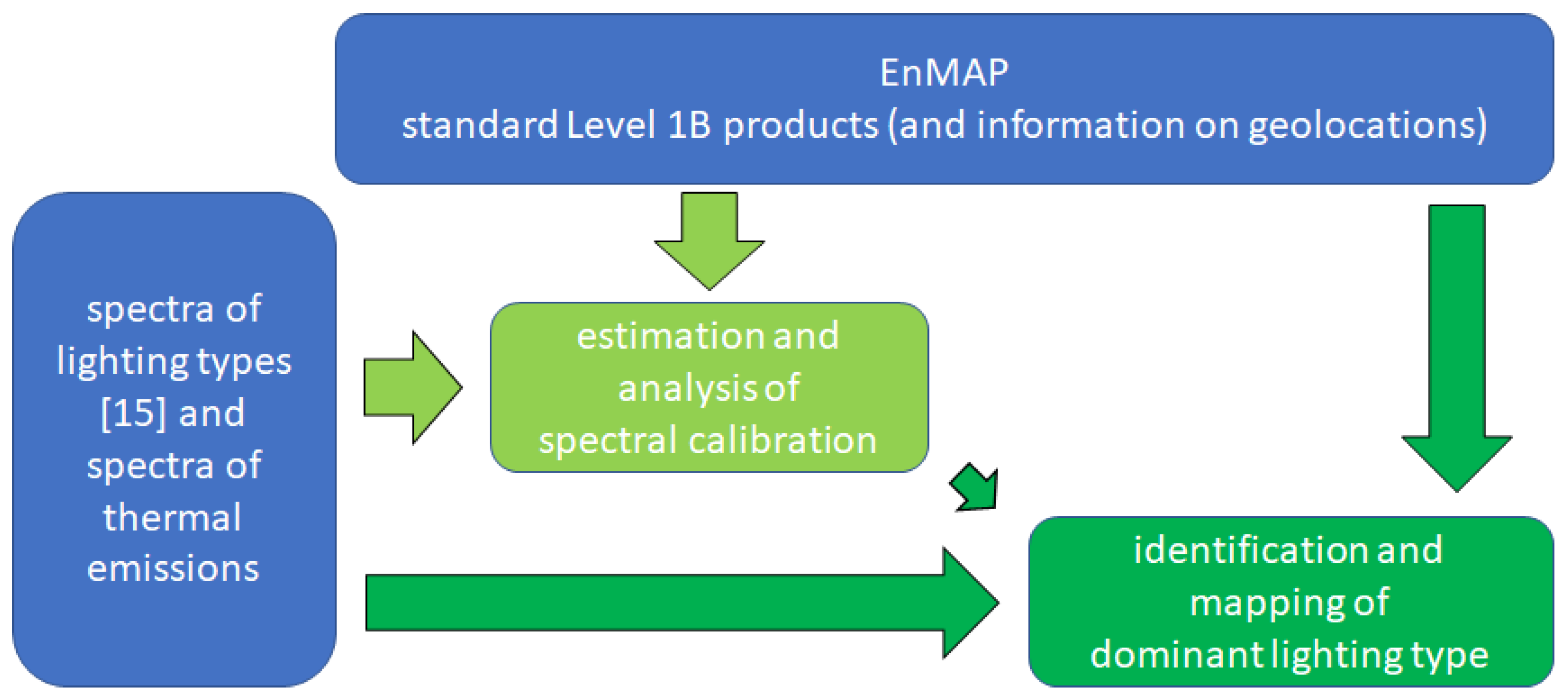
Figure 2.
ColorInfraRed (CIR) composite (red: 863.4 nm, green: 647.3 nm, blue: 550.5 nm) of an orthorectified EnMAP daytime observation (left; (a)) and a color table presentation (red–green–blue: high signal to low signal) of the integrated VIS/NIR signal of the orthorectified EnMAP nighttime observation (right; (b)). The grid lines refer to the standard and north-aligned UTM Zone 11 coordinate grid in WGS 84 with a raster size of 3km in both directions (x-axis state geographic longitude and UTM easting in meters and y-axis state geographic latitude and UTM northing in meters). EnMAP data © DLR 2022. All rights reserved.

Figure 3.
Integrated signals of VIS/NIR (left; (a)) and SWIR (right; (b)) of the EnMAP nighttime observation in sensor geometry, with the non-linear stretch applied. The area covered is approximately . EnMAP data © DLR 2022. All rights reserved.
Figure 3.
Integrated signals of VIS/NIR (left; (a)) and SWIR (right; (b)) of the EnMAP nighttime observation in sensor geometry, with the non-linear stretch applied. The area covered is approximately . EnMAP data © DLR 2022. All rights reserved.
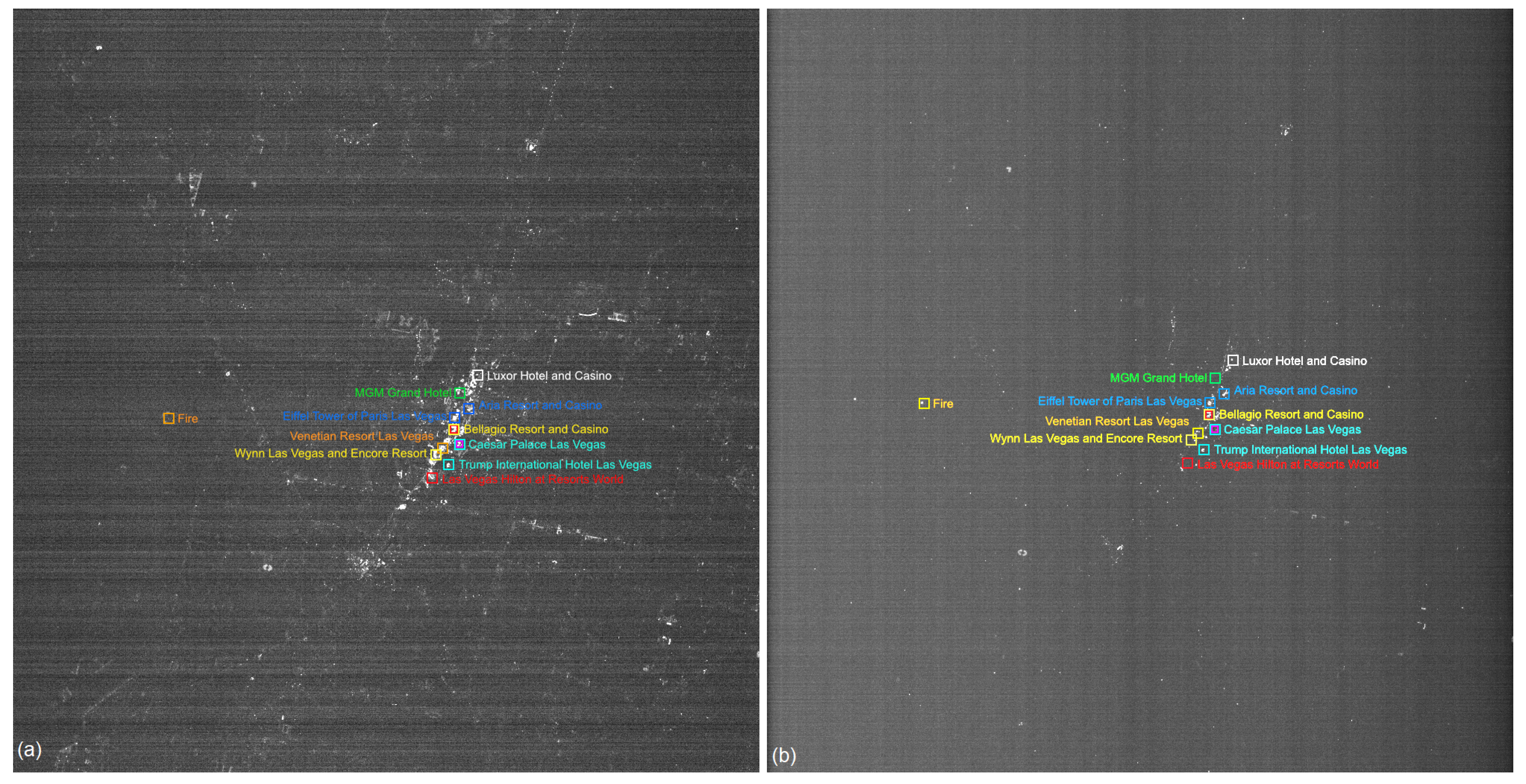
Figure 4.
Seven HPS, MH, and LPS spectra at a resolution of 1 nm for VIS/NIR (top; (a)) and SWIR (bottom; (b)) in the considered ranges; the sum of the signals normalized to 1.
Figure 4.
Seven HPS, MH, and LPS spectra at a resolution of 1 nm for VIS/NIR (top; (a)) and SWIR (bottom; (b)) in the considered ranges; the sum of the signals normalized to 1.

Figure 5.
Atmospheric transmission of an urban mid-latitude summer atmosphere at nadir with three considered water vapors for VIS/NIR (top; (a)) and SWIR (bottom; (b)) in the considered ranges.
Figure 5.
Atmospheric transmission of an urban mid-latitude summer atmosphere at nadir with three considered water vapors for VIS/NIR (top; (a)) and SWIR (bottom; (b)) in the considered ranges.

Figure 6.
HPS reference spectrum at a resolution of 1 nm and spectra at the EnMAP resolution for different VIS/NIR shifts (a) and SWIR (b); the sum of the signals normalized to 1.
Figure 6.
HPS reference spectrum at a resolution of 1 nm and spectra at the EnMAP resolution for different VIS/NIR shifts (a) and SWIR (b); the sum of the signals normalized to 1.

Figure 7.
Image and reference spectra for the scenarios when using the center pixel, the pixel with the maximum signal, the sum of the signals of all pixels, and the optimum pixel for VIS/NIR (top; (a)) and SWIR (bottom; (b)); the sum of the signals normalized to 1.
Figure 7.
Image and reference spectra for the scenarios when using the center pixel, the pixel with the maximum signal, the sum of the signals of all pixels, and the optimum pixel for VIS/NIR (top; (a)) and SWIR (bottom; (b)); the sum of the signals normalized to 1.

Figure 8.
Influence of the number of pixels on the optimum approach. Fitting error (a,b,e,f) as well as estimated shift (in nm) (c,d,g,h) (y-axis) considering a smaller (a–d) or larger (e–h) amount of summed image spectra (x-axis) for VIS/NIR (left; a,c,e,g), and SWIR (right; b,d,f,h).
Figure 8.
Influence of the number of pixels on the optimum approach. Fitting error (a,b,e,f) as well as estimated shift (in nm) (c,d,g,h) (y-axis) considering a smaller (a–d) or larger (e–h) amount of summed image spectra (x-axis) for VIS/NIR (left; a,c,e,g), and SWIR (right; b,d,f,h).

Figure 9.
Influence of noise on the estimation for VIS/NIR (left; (a)) and SWIR (right; (b)). The differences of the observed shifts compared to the shifts of the related noisy reference spectra given on the x-axis for the observed errors given on the y-axis (see the text for full description). Changes from green to olive and blue to purple illustrate the maximal variety in shifts of the noisy reference spectra resulting in the observed errors and shifts. A full green hue is related to a negative shift of nm and a full blue hue to a positive shift of nm. A full red color illustrates the non-existence of shifts of noisy reference spectra, resulting in the observed errors and shifts.

Figure 10.
Integrated signals in the range of bands with respect to the peaks of the emission at 819 nm for VIS/NIR (left; (a)) and 1139 nm for SWIR (right; (b)), non-linear stretch applied. EnMAP data © DLR 2022. All rights reserved.
Figure 10.
Integrated signals in the range of bands with respect to the peaks of the emission at 819 nm for VIS/NIR (left; (a)) and 1139 nm for SWIR (right; (b)), non-linear stretch applied. EnMAP data © DLR 2022. All rights reserved.

Figure 11.
Per-pixel center wavelengths based on laboratory calibrations, estimated considering the full sensor, and the best-fitted two of four parts, namely, half of the sensor for VIS/NIR (top; (a)) and SWIR (bottom; (b)).
Figure 11.
Per-pixel center wavelengths based on laboratory calibrations, estimated considering the full sensor, and the best-fitted two of four parts, namely, half of the sensor for VIS/NIR (top; (a)) and SWIR (bottom; (b)).

Figure 12.
Identified lighting types and temperatures, where Table 2 and Table 3 state the color mappings, based on VIS/NIR (a–d) and SWIR (e,f), where (a,b,e,f) cover the full image, (c,d) cover the Las Vegas Strip, (a,c,e) focus on the identification of general types and (b,d,f) on specific types.

Figure 13.
Observed spectra (solid) and reference spectra by [15] (dashed) for the eight considered image pixels, HPS (a,b), MH (c,d), FL (e), low temperature (f), LPS (g), high temperature (h), for VIS/NIR (left; (a,c,e,g)) and SWIR (right; (b,d,f,h)); the sum of the signals normalized to 1.
Figure 13.
Observed spectra (solid) and reference spectra by [15] (dashed) for the eight considered image pixels, HPS (a,b), MH (c,d), FL (e), low temperature (f), LPS (g), high temperature (h), for VIS/NIR (left; (a,c,e,g)) and SWIR (right; (b,d,f,h)); the sum of the signals normalized to 1.

Figure 14.
Observed spectra (solid) and reference spectra by [15] (dashed) for six considered image pixels, CW (a), NW (b), blue LED (c), green LED (d), red LED (e), yellow LED (f) for VIS/NIR; the sum of the signals normalized to 1.
Figure 14.
Observed spectra (solid) and reference spectra by [15] (dashed) for six considered image pixels, CW (a), NW (b), blue LED (c), green LED (d), red LED (e), yellow LED (f) for VIS/NIR; the sum of the signals normalized to 1.


Table 1.
Uncertainties based on sensitivities and the influences of assumptions A1 to A6. Individual uncertainties affecting the total uncertainty are typeset in bold.
Table 1.
Uncertainties based on sensitivities and the influences of assumptions A1 to A6. Individual uncertainties affecting the total uncertainty are typeset in bold.
| Description | VIS/NIR | SWIR | |
|---|---|---|---|
| sensitivity | to noise | ||
| A1 | lighting types | ||
| A2 | surface types | ||
| A3 | atmospheres | ||
| A4 | range of bands | ||
| A5 | distance metrics | ||
| A6 | image spectra selections | ||
| total | of sensitivity, A1, A2, A3 |
Table 2.
Identified lighting types based on VIS/NIR and SWIR. The error relates to the Euclidean distance of the fit against [15].
Table 2.
Identified lighting types based on VIS/NIR and SWIR. The error relates to the Euclidean distance of the fit against [15].
| Error | Error | ||||
|---|---|---|---|---|---|
| Lighting Type | Color in Figures | VIS/NIR | SWIR | VIS/NIR | SWIR |
| total | 8819 | 451 | 2006 | 448 | |
| HPS | dark blue | 430 | 48 | 165 | 48 |
| MH | light blue | 1479 | 82 | 243 | 82 |
| MV | light green | 20 | 49 | 0 | 48 |
| QH | dark green | 5 | 6 | 0 | 6 |
| FL | orange | 174 | 26 | ||
| LPS | yellow | 8 | 8 | ||
| total LED | magenta | 6658 | 1557 | ||
| CW | cyan | 3311 | 509 | ||
| NW | magenta | 2437 | 740 | ||
| Blue | dark blue | 90 | 0 | ||
| Green | dark green | 69 | 1 | ||
| Red | dark red | 69 | 2 | ||
| Yellow | yellow | 682 | 305 | ||
| total INC/LIQ/PRES | dark red (VIS/NIR) | 45 | 111 | 15 | 108 |
| INC | magenta (SWIR) | 45 | 24 | 15 | 21 |
| LIQ | light magenta (SWIR) | 0 | 11 | 0 | 11 |
| PRES | dark magenta (SWIR) | 0 | 76 | 0 | 76 |
| Temperature | red-orange-yellow (SWIR) | 155 | 155 | ||
Table 3.
Estimated temperatures based on SWIR. The error relates to the Euclidean distance of the fit against emissions based on Planck’s law, separating and not separating the identified INC/LIQ/PRES.
Table 3.
Estimated temperatures based on SWIR. The error relates to the Euclidean distance of the fit against emissions based on Planck’s law, separating and not separating the identified INC/LIQ/PRES.
| Error , Separate Temperature and INC/LIQ/PRES | Error , Separate Temperature and INC/LIQ/PRES | ||||
|---|---|---|---|---|---|
| Temperature (K) | Color in Figures | Yes | No | Yes | No |
| 500 | red | 0 | 0 | 0 | 0 |
| 700 | red-orange | 1 | 1 | 1 | 1 |
| 900 | red-orange | 2 | 2 | 2 | 2 |
| 1100 | red-orange | 14 | 14 | 14 | 14 |
| 1300 | red-orange | 25 | 26 | 25 | 25 |
| 1500 | orange | 31 | 53 | 31 | 52 |
| 1700 | orange-yellow | 15 | 70 | 15 | 65 |
| 1900 | orange-yellow | 24 | 86 | 24 | 69 |
| 2100 | orange-yellow | 12 | 63 | 12 | 57 |
| 2300 | orange-yellow | 8 | 49 | 8 | 48 |
| 2500 | yellow | 23 | 87 | 23 | 84 |
Disclaimer/Publisher’s Note: The statements, opinions and data contained in all publications are solely those of the individual author(s) and contributor(s) and not of MDPI and/or the editor(s). MDPI and/or the editor(s) disclaim responsibility for any injury to people or property resulting from any ideas, methods, instructions or products referred to in the content. |
© 2023 by the authors. Licensee MDPI, Basel, Switzerland. This article is an open access article distributed under the terms and conditions of the Creative Commons Attribution (CC BY) license (https://creativecommons.org/licenses/by/4.0/).
Share and Cite
MDPI and ACS Style
Bachmann, M.; Storch, T. First Nighttime Light Spectra by Satellite—By EnMAP. Remote Sens. 2023, 15, 4025. https://doi.org/10.3390/rs15164025
AMA Style
Bachmann M, Storch T. First Nighttime Light Spectra by Satellite—By EnMAP. Remote Sensing. 2023; 15(16):4025. https://doi.org/10.3390/rs15164025
Chicago/Turabian StyleBachmann, Martin, and Tobias Storch. 2023. "First Nighttime Light Spectra by Satellite—By EnMAP" Remote Sensing 15, no. 16: 4025. https://doi.org/10.3390/rs15164025
Note that from the first issue of 2016, this journal uses article numbers instead of page numbers. See further details here.