Improved On-Orbit MTF Measurement Method Based on Point Source Arrays

Abstract

The modulation transfer function (MTF) is a key characteristic used to assess the performance of optical remote sensing satellite sensors. MTF detection can directly measure a sensor’s two-dimensional (2D) point spread function (PSF); therefore, it has been applied to various high-resolution remote sensing satellites (e.g., Pleiades) using point sources. However, current point source methods mainly use 2D Gaussian functions to fit the discrete digital number (DN) of the point source on the image to extract the center of the point source and fit the PSF after encrypting multiple point sources; thus, noise robustness is poor and measurement accuracy varies widely. In this study, we developed a noise-resistant on-orbit MTF detection method based on the object space constraint among point source arrays. Utilizing object space constraint relationships among points in a point source array, a homography transformation model was established, enabling accurate extraction of sub-pixel coordinates for each point source response. Subsequently, aligning the luminosity distribution of all point sources concerning a reference point source, the encrypted PSF was obtained and then fitted to obtain the MTF. To validate the method, Gaofen-2 (GF-2) satellite images were used to conduct an in-orbit imaging experiment on the point source array of the Chinese Zhongwei remote sensing satellite calibration site. Compared with the Gaussian model methods, the proposed method yielded more accurate peak positions for each point source. Standard deviations of peak position constant ratios in along- and cross-track directions improved by 2.8 and 4.8 times, respectively. The root-mean-square error (RMSE) of the collinearity test results increased by 92%, and the noise resistance of the MTF curve improved by two times. Dynamic MTF values at the Nyquist frequency for the GF-2 panchromatic band in along- and cross-track directions were 0.0476 and 0.0705, respectively, and MTF values in different directions were well distinguished.

1. Introduction

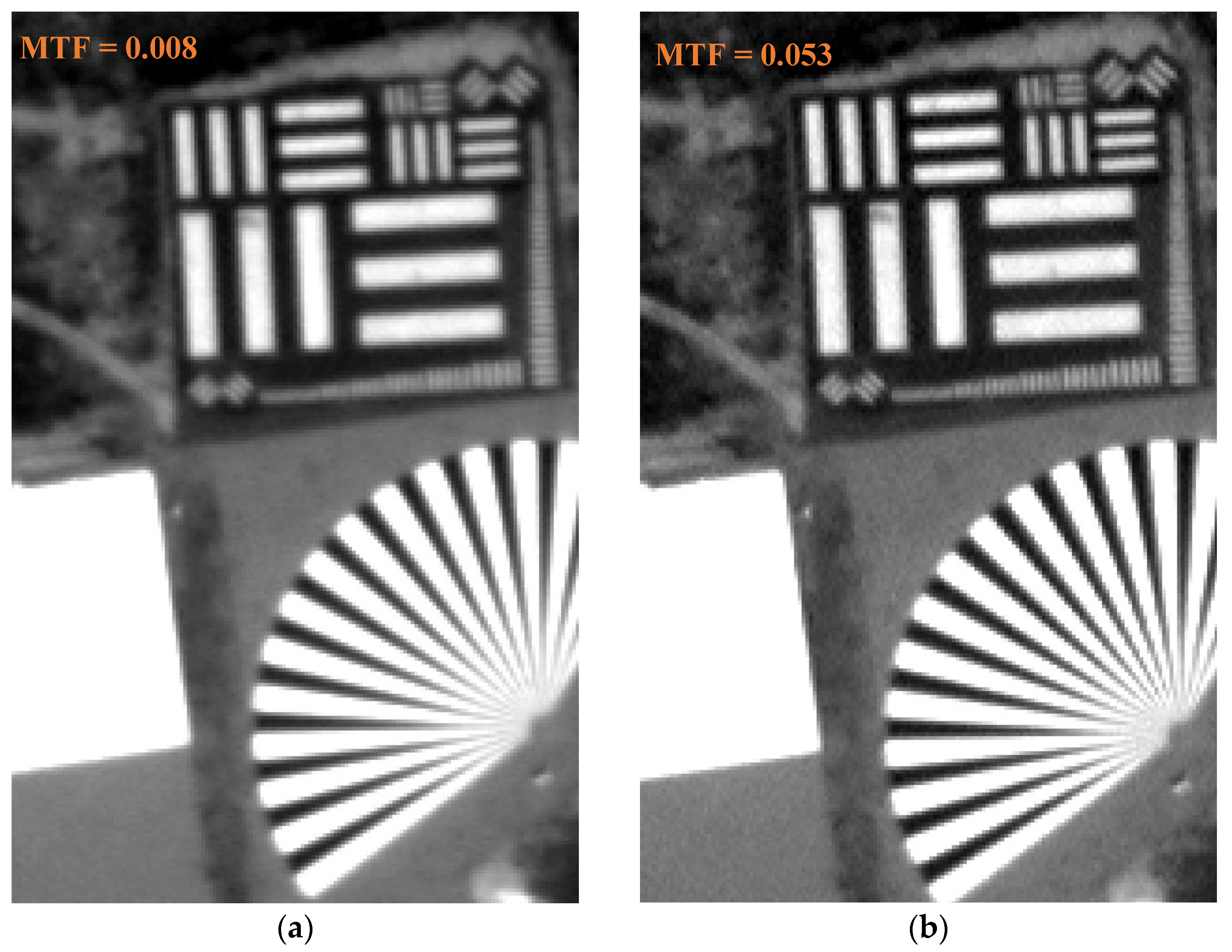
The modulation transfer function (MTF) is a measure of the response of an optical imaging system to different spatial frequency signals of objects and is an important indicator for evaluating the imaging quality of optical satellite sensors. In remote sensing images, the MTF describes the smallest discernible details in the image. A higher MTF value indicates that the system can transmit higher spatial frequency information, which implies that it can capture finer details and provide higher clarity and spatial resolution [1], as shown in Figure 1, which expands the application range of remote sensing imagery.

Prior to the launch of a remote sensing satellite, the sensors are subjected to detailed performance tests in the laboratory, including the MTF values. However, the aging of remote sensor electronic components caused by vibrations during satellite launch and the space environment in orbit (ultraviolet [UV] irradiation, temperature changes, etc.) causes the image quality of sensors to be degraded. Dynamically variable imaging conditions (such as atmospheric transparency, turbulent refraction, and aerosols) can also degrade the image’s MTF. To ensure the quality of remote sensing data, periodic dynamic MTF measurements and compensation are required during the on-orbit operation of satellites [2]. On-orbit MTF measurements are primarily achieved using artificial targets or natural features with special imagery shapes, such as knife-edge targets, roofs, bridges, etc. Given the differences in target types, multiple types of MTF measurements have been developed, including the knife-edge [3,4], pulse [5,6], point source [7,8], and radial target [9,10] methods.

On-orbit MTF detection methods based on slanted knife-edge targets are widely employed in current practice. The knife-edge method samples and fits the knife-edge remote sensing image to obtain the edge spread function (ESF), then derives the line spread function (LSF) and finally the system MTF by Fourier transform and normalization [11,12]. The advantage is that the choice of targets is diverse, including both natural features, such as the moon [13] and glacier edges [14], and manually placed targets. However, because the edge itself does not contain multiple frequency components, it is necessary to recover the various frequencies from the extracted edge spread function, which inevitably introduces noise and additional errors, thereby reducing the accuracy of MTF detection [4]. The pulsed method of on-orbit MTF detection is mainly extracted from remote sensing images of bridges, airport runways, and other linear features to fit the line spread function. Then, the ratio of the Fourier transform is performed to obtain the MTF [6,15]. The advantages are that the selection of natural features is more intuitive, and the background noise is less influential, which makes it easy to obtain reliable results. The disadvantages are that there is no possibility of setting ideal ground targets because of the different resolutions of different satellites, and it takes a long time to find the pulsed natural features in a fixed direction. According to the definition of MTF, when an optical satellite camera images a radiation target at a certain frequency, the ratio of the output (measured image space) signal amplitude to the input (target object space) signal amplitude is the MTF at the frequency. However, only a single MTF value at the high frequency (i.e., the Nyquist frequency) can be obtained. Although sufficient statistical averaging can improve the accuracy of MTF detection, the process is susceptible to atmospheric influence, resulting in a certain dispersion of the detection results [10].

The point source method is based on the physical definition of the MTF and is theoretically the most tightly defined optical sensor on-orbit MTF detection method capable of directly acquiring the two-dimensional (2D) point spread function (PSF). The image of the scene viewed by the sensor is not a completely faithful reproduction, and small details are blurred relative to larger features (Figure 2a,b); this blurring is characterized by the total sensor PSF [16]. Mathematically, it can be considered as the convolution of the sensor PSF with the input signal. Therefore, the MTF of the system in any direction can be obtained by Fourier transform of the PSF (Figure 2b,c). Some of the point source targets that can be used include deep-space stars [17,18], active point targets [19], black squares on white sand surfaces [20], and convex mirrors [21]. Remote sensing imaging systems have different response characteristics at various spatial locations and directions [21], and so single-point source targets not sampled with sufficient points are vulnerable to the influence of the surrounding ground radiation and atmospheric state, resulting in low accuracy of the measurement results. To improve the accuracy and stability of MTF measurements, the PSF is typically reconstructed by combining multiple point sources, as shown in Figure 3.

When point targets are imaged in the sensor, the central peak radiometric response of each point source cannot be located exactly at the positive center of the sensor PSF owing to the limitation of satellite’s orbit, pointing accuracy, and attitude stability, and most cases are imaged at sub-pixel locations off the positive center of the PSF. When multiple point sources are imaged, if the peak position of each point source is inaccurate, then the reconstructed PSF with peak alignment is also incorrect and the assessed MTF results are unreliable. Therefore, an accurate and effective method to solve the peak position is required to achieve the high-precision reconstruction of the PSF from multiple point sources and ensure the accuracy of the MTF evaluation. There are two categories of image processing methods for extracting the sub-pixel coordinates of peak radiometric response: target grayscale and target edge information. The first category is the center localization method, which is based on target grayscale and includes Gaussian fitting [21], centroid localization [22], and centroid-weighted localization [23]. Among the three methods, Gaussian fitting is the most effective. Therefore, it is commonly applied in various satellite systems, such as Quickbird [21] and ZY-3 [24]. The second category is based on target edge information, and it employs edge circle fitting [25] and the Hough transform [26]; these methods are mainly used in star extraction applications.

Multiple point sources contain redundant information, such as the geometric constraints in the point source array. By purifying sub-pixel positions of the point sources using geometric constraints, noise interference can be effectively avoided. Therefore, by leveraging object space geometric constraints such as coplanarity and equidistance between ground point sources, it is possible to accurately extract the peak response positions of point sources and improve the accuracy of MTF detection. In this study, we developed a noise-resistant on-orbit MTF detection method based on the object space constraint between point source arrays. By establishing a homography transformation model from the object space to the image space based on the geometric constraints of the point source array, the peak response coordinates of each point source could be accurately extracted; the extraction results were comparable with those of traditional Gaussian methods. The brightness distributions of all the point sources were aligned with the reference point sources, fitted, and calculated to obtain the PSF and MTFs. Finally, the MTF calculation results were simulated for different noise conditions, and the point source arrays of the Gaofen-2 (GF-2) satellite and Chinese Zhongwei remote sensing satellite calibration site were used for on-orbit imaging test verification.

The remainder of the paper is arranged as follows: Section 2 provides a comprehensive account of the placement of the array target, optimization of peak position detection, and MTF calculation. The calibration tests site and data presentation are described in Section 3. In Section 4, we present the effects of sub-pixel extraction, combined experiments on the MTF detection results and noise simulations, and a comparison of all tested methods using quantitative assessments. Finally, Section 5 and Section 6 discuss the potential problems and provide our research conclusions.

2. Methods

The array point source method is a technique of direct detection to evaluate on-orbit MTF based on the physical definition of MTF. Reflective point sources with non-integer pixel intervals were deployed in both the along- and cross-track directions during the flight of the satellite remote sensing system. These sources formed a cyclic matrix to obtain the PSF and MTF of the imaging system [27,28,29]. Utilizing the geometric constraints of the fixed arrangement of the point source array in the object space, a homography transformation model was used to align the encrypted brightness responses with PSF fitting and MTF calculation, as shown in Figure 4.

2.1. Point Source Array Design

According to the sensor PSF measurement principle, to accurately measure the PSF the point source sampling of the sensor PSF needs to satisfy the following: (1) all sampling points of the sensor imaging can cover a PSF uniformly; (2) sampling points along the along- and cross-track directions are equally spaced and co-lined (as shown in Figure 5a); and (3) there should be a sufficient number of sampling points to adequately sample the PSF (as shown in Figure 5b). Therefore, the interval between adjacent sampling points can be determined using the equation:

$$\mathrm{∆}x=m+\frac{1}{n},$$

(1)

where m is the number of integer pixels and n is the number of sampling points along the along- or cross-track direction.

To ensure that the solar radiation is similar when remote sensing satellites observe the same area many times, the orbits of remote sensing satellites are mostly designed as sun-synchronous orbits with a certain inclination φ. At this time, the angle $\theta \approx \phi -90°$ exists between the along-track direction of the satellite’s Earth observation and the due north direction of the ground. To ensure that the array columns of the point source array are aligned with the along-track direction of the satellite during actual deployment, the angle between the array rows and true north must be designated as θ, as shown in Figure 6. This is necessary because different remote sensing satellites have different orbit inclinations. To reduce the hardware requirements, sensors are typically designed as a combination of panchromatic and multispectral bands. The panchromatic band captures high-resolution information on the Earth’s surface, whereas the multispectral band provides spectral information. The resolution ratio is generally 1:4. To facilitate the on-orbit MTF testing of both panchromatic and multispectral payloads, the point source array needs to be designed separately for each. As shown in Figure 5, 25-point source devices were arranged in a 4 × 4 array in the panchromatic region and a 3 × 3 array in the multispectral region. The spacing between adjacent point sources, denoted as Δx, was as follows:

$$\mathrm{∆}x=m+0.25$$

(2)

In mobile deployment mode, it is difficult to meet the demand for regular calibration because of the low efficiency of manual deployment and reflector pointing during the on-orbit test. It is advisable to use the fixed deployment mode since it enables the MTF measurement test to be performed in orbit automatically without human supervision.

2.2. Peak Position Detection

Homographic transformation is a type of projection transformation that maps one plane to another while preserving straight lines and parallel relationships within the plane [30]. Remote sensing imaging is the process of converting radiometric energy information from the Earth’s surface to digital images on an image plane. Geometric distortions in image shape and position can occur owing to factors such as inaccurate sensor installation, changes in the Earth’s surface, and non-ideal characteristics of the optical system. The rational polynomial coefficients (RPC) model, commonly used for correcting geometric distortions, is not completely accurate in small-scale regions [31]. Residual errors that persist after correction include imaging distortions such as object-to-image plane orientation transformation and resolution inconsistencies. It is possible to simplify these somewhat-complex transformations into homographic transformations that are relatively simple. Remote sensing imaging can project the ground point source array onto the image plane, establishing an eight-degrees-of-freedom homography matrix that describes the mapping relationship between the two planes. The homographic transformation can correct the projection of ground points onto the image plane. The collinearity and coplanarity constraints embedded within the homography mapping relationship can rectify distortions in the projection of ground points onto the image plane. This is illustrated in Figure 7.

The mathematical expression of the homography matrix is:

$$q^a\propto H_{ }{q}^b$$

(3)

which can be expanded as:

$$\left[\begin{array}{c}{u}_a\\ v_a\\ 1\end{array}\right]\propto \left[\begin{array}{ccc}{H}_1& H_2& H_3\\ H_4& H_5& H_6\\ H_7& H_8& H_9\end{array}\right] \left[\begin{array}{c}{u}_b\\ v_b\\ 1\end{array}\right]$$

(4)

where the positive ratio to sign $\propto$ can be interpreted as the homography matrix constraining the directions of $q^a$ and $H_{ }{q}^b$ in the same direction without constraining the scale. The scale factor of the chi-square can be eliminated by the fork product calculation; therefore, the above constraint can also be expressed in the following form:

$$q^a\times H_{ }{q}^b=0$$

(5)

As $q^a$ and $H_{ }{q}^b$ are in the same direction, the result of their fork multiplication is a zero vector.

The following is the specific implementation method for detecting peak positions, taking into account homographic transformation. By utilizing the ground coordinates provided by the point source devices, along with the initial RPC model generated from the imagery, it is possible to compute the image coordinates of the points. Furthermore, the RPC model provides better adaptation to image data with varying resolutions and angles. The peak coordinates of the initial point source, calculated using the RPC model, remain unaffected by image noise, ensuring the relatively accurate absolute spatial position of the initial peak coordinates. However, it should be noted that each point is extracted separately and, although it inherits part of the object space geometric relationship, it still differs significantly from the coplanar and equally spaced geometric relationship in the ground design.

To re-establish stable geometric relationships, such as collinearity and parallelism among the peak coordinates of the image, the initial peak coordinates obtained from the RPC solution were subjected to homographic transformation using the homography matrix. As a result of this transformation, the peak coordinates regained a stable geometric relationship between collinearity and parallelism.

When the object space coordinates Q₁ correspond perfectly to the image space coordinates Q₂, there exists a homography matrix H, which can be obtained from Equation (4).

$$Q_2=H\times Q_1$$

(6)

However, an error occurred when the image square coordinates of the RPC orthographic projection were first applied. Therefore, first, RANSAC [32] was employed to identify and eliminate unreasonable matching points, thereby improving the accuracy and reliability of the homography matrix. Second, the least squares overdetermined system of equations was applied to solve H to obtain the transformation relation H_m from the object space to the image space, and the optimized peak coordinates were from Equation (7) as follows:

$$Q_{2\_repair}=H{\_}_m\times Q_1$$

(7)

Thus, by mapping the object coordinates to the same image plane, the correction of the initial peak coordinates could be achieved, as shown in Figure 8.

2.3. MTF Calculation

The point source region within the remote sensing image is analyzed by sequentially extracting each point source’s data while using the peak response coordinates, as calculated in Section 2.2, as reference coordinates. Each point source is then moved to the origin of the 3D coordinate plane to obtain the system’s PSF profile. The optical satellite imaging system’s point spread characteristics to a point source target are typically explained by a two-dimensional Gaussian model that considers the system noise and background response. Therefore, the system’s response to the point source target is expressed as:

$$g\left(x,y\right)=k exp\left[-\frac{{\left(x-x_0\right)}^2}{2{\sigma }^2}-\frac{{\left(y-y_0\right)}^2}{2{\zeta }^2}\right]+b$$

(8)

where k is the coefficient factor, $\left(x_0,y_{0,}\right)$ is the peak response (i.e., image point coordinates), σ and ζ are the standard errors, and b is the background value.

The PSF of the satellite camera’s imaging system is determined through the least squares fitting method. Fourier transform, taking the mode, and normalization can be used to characterize the spatial frequency response characteristics of this satellite optical sensor MTF, which can be expressed as:

$$MTF\left(u,v\right)=\frac{\left|FT\left|g\left(x,y\right)\right|\right|}{\left|F{T}_{u,v=0}\left|g\left(x,y\right)\right|\right|}$$

(9)

where $FT| |$ is the Fourier transform and $| |$ denotes the mode taken [8,24].

3. Calibration Tests and Data Presentation

The Zhongwei remote sensing satellite calibration site is a fully automated integrated calibration site jointly established by the Zhongwei Municipal Government, Wuhan University, and Beijing Aerospace Yuxing Technology Co., Ltd. It is equipped with reflective point source targets, synthetic aperture radar (SAR) active calibrators, SAR automatic angle reflectors, laser geometric calibrators, and other equipment that can perform on-orbit calibration for visible light, SAR, and laser altimetry. The distribution of targets is shown in Figure 9.

Reflective point source equipment mainly consists of combined convex mirrors, solar sensors, attitude control components, and shields. According to the dynamic range of the sensor, the reflective point source target that reflects the appropriate amount of luminous flux in the high end of the response of the satellite optical camera is not saturated. According to the accuracy of satellite orbit prediction and reflective point source pointing accuracy, etc., to ensure that the sensors at the time of the top of the solar beam are reflected by the point source, the design of the mirror scale is <10% of the resolution of the ground image of the sensor to achieve a lightweight, miniaturized. Through automatic tracking and observation of the sun’s trajectory by the solar sensitizer, the calibration of the point source position control error and angular scale can be achieved with an accuracy of better than 0.1°, and the optical path between the sunlight point source target optical remote sensing satellites can be automatically adjusted to accurately obtain the remote sensing image of the ground-reflected point source [33].

Point light source equipment has a wide range of satellite resolution (e.g., panchromatic camera 0.5–1 m, multispectral camera 2–4 m); therefore, the site has a 16-point light source 4 × 4 array layout for panchromatic cameras and a 9-point light source 3 × 3 array for multispectral cameras. The 25 sets of reflective point light source targets form an array of point light sources with multi-level brightness levels that reflect sunlight into the satellite camera pupil and perform absolute radiometric calibration and MTF detection of high-resolution optical remote sensing satellite sensors for radiometric performance and image quality assessment. Figure 10 shows the ground-based point source targets turned on during satellite–ground simultaneous observation tests. Each reflective point source target was installed and measured with high precision using RTK (real-time kinematic) technology to obtain objects’ space coordinates. The 4 × 4 rectangular point source array is numbered in sequential order from west to east and from north to south as P1, P2, …, P15, and P16.

The GF-2 satellite is the second satellite in China’s Gaofen series. It was launched in August 2014 and carries a panchromatic medium-resolution sensor (PMS) capable of capturing 1 m panchromatic black-and-white images and 4 m multispectral color images (

Table 1. Gaofen-2 satellite sensor basic information.

Resolution (m)	Bands	Tag
		Wavelength (μm)	Swath Width (km)	Lateral Swing Angle (°)
1.0 4.0	Panchromatic	0.45–0.90	45	±35
	Multispectral	0.45–0.52, 0.52–0.59, 0.63–0.69, 0.77–0.89	45	±35

). From September to October 2021, GF-2 was used to conduct imaging experiments on the reflective point source array in the Zhongwei Calibration site, successfully capturing image data of the point light source area.

As shown in Figure 11, the panchromatic band of the GF-2 sensor was successfully captured by the point source device, and the radiation response of the 4 × 4 panchromatic region of the point source was normal. The 3 × 3 region was designed for multispectral analysis, and so the response was saturated in the panchromatic band. From Figure 11, the uniformity of the background region of the Zhongwei Point light source site needs to be further improved, as non-uniform errors introduce background noise and uncertainty to PSF profile fitting and MTF solving.

4. Results and Analysis

4.1. Peak Position Detection

The peak position of the RPC orthographic projection was optimized using a homography matrix to obtain the peak position of each reflected point source response; the results are listed in

Table 2. Pixel coordinates of reflected point source images.

Parameter	P1	P2	P3	P4	P5	P6	P7	P8
X0/Pixel	22.8203	22.4905	22.1804	21.8173	64.4319	64.1161	63.6994	63.3783
Y0/Pixel	19.9205	62.0279	103.9604	145.9510	20.3012	62.3427	104.4202	146.3459
Parameter	P9	P10	P11	P12	P13	P14	P15	P16
X0/Pixel	106.0521	105.6723	105.3178	104.9998	147.7732	147.3949	146.9973	146.5499
Y0/Pixel	20.7226	62.6444	104.7345	146.7138	20.9637	63.0107	105.0956	147.0431

. X₀ and Y₀ are the relative pixel coordinates of the peak position, and P_i denotes different point sources; i = 1, 2, 3, …, 16.

To verify the accuracy and stability of the peak response coordinates of the proposed method, the scale constants and peak response coordinate co-linearity of the proposed method were compared with that of the 2D Gaussian model method in the optical remote sensing sensor.

When the same sensor of an optical remote sensing satellite images two reflected point source targets on the ground, the ratio of the ground spacing of the point source target to the image spacing of its corresponding satellite remote sensing image is constant according to the imaging geometric relation. Accordingly, the image point coordinates extracted from each reflected point source image can be used to obtain the image point spacing, and the proportionality constant of the sensor can be obtained using the corresponding ground spacing [34]. The corrected scale constants of the proposed method were compared with those of the 2D Gaussian model to determine the peak position detection results, as shown in

Table 3. Results of scale checkout.

Cross-Direction			Along-Direction
Segment	This Study	Gaussian Fit	Segment	This Study	Gaussian Fit
P1–P5	0.7990	0.8005	P1–P2	0.7907	0.7927
P1–P9	0.7987	0.7984	P1–P3	0.7910	0.7911
P1–P13	0.7984	0.8010	P1–P4	0.7913	0.7912
P2–P6	0.7993	0.8021	P2–P3	0.7913	0.7896
P2–P10	0.7990	0.7991	P2–P4	0.7917	0.7905
P2–P14	0.7987	0.8008	P3–P4	0.7920	0.7914
P3–P7	0.7996	0.8010	P5–P6	0.7904	0.7915
P3–P11	0.7993	0.7989	P5–P7	0.7907	0.7908
P3–P15	0.7991	0.8010	P5–P8	0.7910	0.7912
P4–P8	0.8000	0.7985	P6–P7	0.7904	0.7901
P4–P12	0.7997	0.7992	P6–P8	0.7914	0.7911
P4–P16	0.7994	0.7999	P7–P8	0.7911	0.7920
P5–P9	0.7984	0.7962	P9–P10	0.7917	0.7876
P5–P13	0.7981	0.8013	P9–P11	0.7904	0.7909
P6–P10	0.7987	0.7960	P9–P12	0.7908	0.7902
P6–P14	0.7985	0.8001	P10–P11	0.7908	0.7943
P7–P11	0.7991	0.7969	P10–P12	0.7911	0.7915
P7–P15	0.7988	0.8011	P11–P12	0.7901	0.7888
P8–P12	0.7994	0.7999	P13–P14	0.7908	0.7926
P8–P16	0.7991	0.8005	P13–P15	0.7902	0.7905
P9–P13	0.7979	0.8064	P13–P16	0.7905	0.7914
P10–P14	0.7982	0.8042	P14–P15	0.7914	0.7885
P11–P15	0.7985	0.8053	P14–P16	0.7908	0.7908
P12–P16	0.7988	0.8011	P15–P16	0.7911	0.7931
Average	0.7989	0.8004	Average	0.7909	0.7910
SD	0.0005	0.0024	SD	0.0005	0.0014
Relative SD	6.4‱	30.5‱	Relative SD	6.0‱	18.1‱

. A comparative analysis showed that the consistency of the average proportionality constants reflected the accuracy of the sensor probes. The standard deviation (SD) of the scaling constant based on the proposed method was 0.05% in both the along- and cross-track directions, which is 2.8 and 4.8 times higher than that of the 2D Gaussian model in the along- and cross-track directions, respectively; the relative deviations were 4.8 and 3.0 times higher, respectively, indicating the high stability of the proposed method for peak position detection.

In the array point source method of image quality evaluation test, the ground point source equipment in the deployment of the principle of the common line, the target center of the lateral or longitudinal line, should be in a straight line, according to the common line test; the sum of the distance of adjacent reflective point source centers should be equal to the distance between the centers of non-adjacent reflective point sources. As shown in

Table 4. Co-linear relationships.

Cross-Direction			Along-Direction
Co-Linear Relationship	This Study	Gaussian Fit	Co-Linear Relationship	This Study	Gaussian Fit
P1P5 + P5P9 − P1P9	9.9036 × 10−6	7.7094 × 10−6	P1P2 + P2P3 − P1P3	2.0096 × 10−6	2.6332 × 10−5
P1P5 + P5P13 − P1P13	2.0004 × 10−5	4.8339 × 10−5	P1P2 + P2P4 − P1P4	5.0257 × 10−7	1.7508 × 10−4
P1P9 + P9P13 − P1P13	2.0699 × 10−4	8.3285 × 10−5	P1P3 + P3P4 − P1P4	1.4951 × 10−5	3.0898 × 10−4
P2P6 + P6P10 − P2P10	9.5744 × 10−7	1.0652 × 10−4	P2P3 + P3P4 − P2P4	1.6458 × 10−5	1.6024 × 10−4
P2P6 + P6P14 − P2P14	2.9097 × 10−6	2.8449 × 10−5	P5P6 + P6P7 − P5P7	6.0001 × 10−5	1.1704 × 10−5
P2P10 + P10P14 − P2P14	2.5993 × 10−5	5.2544 × 10−5	P5P6 + P6P8 − P5P8	2.2607 × 10−5	1.9410 × 10−6
P3P7 + P7P11 − P3P11	1.2892 × 10−4	2.1647 × 10−4	P5P7 + P7P8 − P5P8	1.5339 × 10−5	9.9237 × 10−6
P3P7 + P7P15 − P3P15	1.2189 × 10−4	5.3958 × 10−7	P6P7 + P7P8 − P6P8	5.2732 × 10−5	1.9687 × 10−5
P3P11 + P11P15 − P3P15	5.8272 × 10−6	5.8321 × 10−4	P9P10 + P10P11 − P9P11	4.2557 × 10−6	5.2724 × 10−6
P4P8 + P8P12 − P4P12	4.5416 × 10−6	9.8819 × 10−5	P9P10 + P10P12 − P9P12	1.5713 × 10−5	6.9554 × 10−6
P4P8 + P8P16 − P4P16	1.7302 × 10−5	3.8845 × 10−5	P9P11 + P11P12 − P9P12	1.9010 × 10−5	8.5169 × 10−5
P4P12 + P12P16 − P4P16	2.1444 × 10−5	2.266 × 10−5	P10P11 + P11P12 − P10P12	7.5529 × 10−6	8.3486 × 10−5
P5P9 + P9P13 − P5P13	1.9689 × 10−4	4.2655 × 10−5	P13P14 + P14P15 − P13P15	2.1216 × 10−6	2.0078 × 10−4
P6P10 + P10P14 − P6P14	2.4041 × 10−5	1.3061 × 10−4	P13P14 + P14P16 − P13P16	1.5699 × 10−5	1.8198 × 10−4
P7P11 + P11P15 − P7P15	1.2853 × 10−5	7.9914 × 10−4	P13P15 + P15P16 − P13P16	2.9229 × 10−5	5.8349 × 10−6
P8P12 + P12P16 − P8P16	8.6829 × 10−6	8.2634 × 10−5	P14P15+P15P16 − P14P16	1.5651 × 10−5	2.4634 × 10−5
Average	5.0572 × 10−5	1.4640 × 10−4	Average	1.8365 × 10−5	8.1750 × 10−5
RMSE	1.8542 × 10−5	2.5497 × 10−4	RMSE	4.7956 × 10−6	1.1790 × 10−4

, the maximum error of the co-linearity test can represent the stiffness and stability of the sensor probe element within the range of the sensor probe element being measured. The error of the improved sensor co-linearity test was <0.03% of a pixel in both the along- and cross-track directions, and the maximum error of the co-linearity test results of the 2D Gaussian fit method of image point extraction was 0.08% of a pixel, which proves the consistency of the sensor probe elements of the two methods. Using the ground actual deployment of the array point source device co-linearity for comparison, its root-mean-square error (RMSE) improved by 92%, indicating that the improved method of array point source image extraction for accuracy and precision has been greatly improved.

4.2. MTF Calculation

Using the point source array peak position coordinates, a meticulous sub-pixel registration process was performed on the data within a 7 × 7 pixel window surrounding each peak position. This approach allows the acquisition of an exquisite sub-pixel system point spread response, which elegantly describes the point spread profile characteristics of a satellite-based remote sensing imaging system [7]. As shown in Figure 12, the system PSF can be obtained by fitting a 2D Gaussian model, eliminating the points with excessive residuals. The goodness of fit is greater than 0.99, which is Fourier transformed to obtain the mode and normalized to obtain the imaging system MTF curve, as shown in Figure 13.

To further verify the applicability of the proposed method, the mean square error (MSE) of the MTF curve was calculated by adding random noise with standard deviations of 5, 10, and 15 to the remote sensing images through computer simulations, as shown in Figure 14. Although the magnitude of the MSE was in the order of 10⁻⁴, the proposed method significantly outperformed the conventional Gaussian method. As the standard deviation of the noise increased, the proposed method maintained approximately twice the advantage in terms of MSE. This indicates that the method is robust to noise.

The on-orbit determination of the MTF for the GF-2 optical satellite image shows that the MTF values of the system at the Nyquist frequency in the along- and cross-track directions after optimization of the image point peak position were 0.0476 and 0.07048, respectively, (Figure 13) whereas the MTF values of the system at the Nyquist frequency in the along- and cross-track directions obtained by the conventional Gaussian fitting method were 0.05453 and 0.0594, respectively, (Figure 15a). Figure 15b shows the MTF curves of the system obtained by the knife-edge method. Figure 15c,d show the MTF curves of the three methods in the along- and cross-track directions, respectively. There are noticeable differences in the detection results at the Nyquist frequency between the knife-edge method and the other two methods in both directions. The presence of the ringing artifacts phenomenon in the edge target image (Figure 16a), which is a step phenomenon due to edge overcompensation (Figure 16, red circle), indicates that the knife-edge target image has been processed by the Model Transfer Function Compensation (MTFC) in the ground processing, causing low-frequency elements in the image to decrease, high-frequency elements to increase, and contrast to increase. This significantly improved the calculated MTF value at the Nyquist frequency. Comparing the improved point source method with the traditional Gaussian model fitting point source method, the traditional Gaussian fitting method showed limited discrimination in the MTF, whereas the improved method showed good discrimination in both the along- and cross-track directions, which is consistent with the discrimination of the traditional knife-edge method. This means that the effect of motion blur is to reduce the MTF in the along-track direction.

5. Discussion

The RPC orthographic image point source peak position based on homography transformation correction improves the original point source peak position detection, which is only retrieved from the image spatial principle alone. Therefore, the obtained image point peak coordinates can more accurately represent the image element response peak position, which in turn makes point spread response profile fitting more accurate and finally obtains a more accurate system MTF. Following the trend of increasing spatial resolution of remote sensing images and the miniaturization and automation of ground-based equipment, this solution will facilitate on-orbit MTF measurement of high-resolution sensors.

The background homogeneity of the calibration site of the Zhongwei remote sensing satellite needs to be improved; the shield of the point source equipment is large, which increases the background noise. Influenced by the solar altitude angle at the time of satellite imaging, a shadow of the point source device shield forms on the ground, leading to a higher level of noise interference on the grayscale variation at the pixel scale. This shadow manifests itself in the image as pixels with significantly lower brightness near the peak pixel, as shown in Figure 17a, which is a dark region. When a PSF contour fit is performed for each point source, the shaded pixels show obvious error points, as shown in Figure 17b. Eliminating these error points effectively improves the PSF fit.

The method used in this study, nonlinear least squares, is the dominant technique for PSF fitting. However, this method is highly sensitive to the initial choice of parameters; incorrect initial choices can cause the algorithm to select a local, rather than the desired global, optimal solution. In addition, the complexity of the computations involved and the need for iterations add to the algorithmic complexity and computational cost. Furthermore, factors such as noise can introduce instability or inaccuracy in the fitting results. For future PSF fitting algorithms, automated methods for initial parameter estimation should be explored, rapid and efficient computational strategies should be developed to improve the soundness and robustness of fitting algorithms, and machine learning and deep learning technologies should be used to improve the accuracy and generalization of PSF fitting results, ultimately improving the accuracy of MTF detection.

An analysis of the method proposed in this study shows that it outperforms traditional methods in peak pixel detection. However, owing to the influence of background image noise, the improvement in the accuracy of PSF contour fitting was not significant, resulting in a limited improvement in the MTF detection results. Nevertheless, the RPC orthorectified image provided in this study accurately maintained the absolute positions of the peak coordinates, which, combined with the homographic transformation, improved the relative geometric relationship between the peak coordinates. As the simulated noise increased, the proposed method showed strong noise resistance and clear superiority.

6. Conclusions

This paper proposes a noise-resistant on-orbit MTF detection method based on the object space constraint between point source arrays. This approach overcomes the drawback of analyzing images only from the digital numerical quantization value of image space elements, utilizes the object space constraint relationship between point source arrays, improves the object plane to image plane relationship by homography transformation, constructs and solves the homography matrix to realize the extraction of point source sub-pixel coordinates, increases the reliability of the encrypted PSF, and improves the calculation accuracy of the MTF.

Compared with the Gaussian fitting method, the proposed approach exhibited 2.8 and 4.8 times better performance in the standard deviation of the scale constant in the along- and the cross-track directions, respectively. The root-mean-square error (RMSE) of the collinearity test for peak pixel extraction improved by 92% using the proposed method. In addition, the system MTF values calculated after PSF fitting in the along- and cross-track directions were 0.0476 and 0.07048, respectively, at the Nyquist frequency. These values demonstrate good distinguishability in different directions, enabling a more accurate evaluation of MTF in remote sensing images. Furthermore, when considering simulated random noisy conditions with standard deviations of 5, 10, and 15, the MSE of the MTF curves was on the order of 10⁻⁴, demonstrating that the proposed method exhibits twice the noise resistance of traditional methods. These results confirm the viability of the proposed method for on-orbit MTF detection in high-resolution optical remote sensing satellites and highlight its superiority in peak pixel extraction and noise resistance over traditional methods. Ultimately, this approach enables high-precision and routine on-orbit performance testing of high-resolution optical satellite sensors.