Radar Anti-Jamming Decision-Making Method Based on DDPG-MADDPG Algorithm

Abstract

In the face of smart and varied jamming, intelligent radar anti-jamming technologies are urgently needed. Due to the variety of radar electronic counter-countermeasures (ECCMs), it is necessary to efficiently optimize ECCMs in the high-dimensional knowledge base to ensure that the radar achieves the optimal anti-jamming effect. Therefore, an intelligent radar anti-jamming decision-making method based on the deep deterministic policy gradient (DDPG) and the multi-agent deep deterministic policy gradient (MADDPG) (DDPG-MADDPG) algorithm is proposed. Firstly, by establishing a typical working scenario of radar and jamming, we designed the intelligent radar anti-jamming decision-making model, and the anti-jamming decision-making process was formulated. Then, aiming at different jamming modes, we designed the anti-jamming improvement factor and the correlation matrix of jamming and ECCM. They were used to evaluate the jamming suppression performance of ECCMs and to provide feedback for the decision-making algorithm. The decision-making constraints and four different decision-making objectives were designed to verify the performance of the decision-making algorithm. Finally, we designed a DDPG-MADDPG algorithm to generate the anti-jamming strategy. The simulation results showed that the proposed method has excellent robustness and generalization performance. At the same time, it has a shorter convergence time and higher anti-jamming decision making accuracy.

1. Introduction

In the game between radar and electronic jamming, jammers will constantly change jamming strategies to generate more complex and unpredictable jamming modes [1,2]. This brings serious threats and challenges to radar’s anti-jamming ability [3]. Accurate decision making is a crucial prerequisite for efficient countermeasures in radar anti-jamming [4]. Anti-jamming decision making based on template matching is effective when the radar is faced with simple jamming [5]. When there are only a few ECCMs in the radar knowledge base, using the multi-attribute decision-making method [6] or the fuzzy analytic hierarchy process [7] can also solve the decision-making problem. However, with the rapid development of jamming [8], there are more and more modes of radar ECCMs [9,10,11,12,13]. Traditional decision-making methods cannot meet the need for intelligent anti-jamming for cognitive radar [14]. The idea of reinforcement learning (RL) coincides with the issue of intelligent radar anti-jamming decision making, as it mainly solves sequence decision-making problems [15]. RL has been successfully applied in the field of communication anti-jamming [16,17,18,19]. Therefore, some scholars have attempted to apply RL to the field of radar anti-jamming decision making [20,21,22,23,24].

For frequency agile (FA) radar, Q-learning [25] and deep Q-network (DQN) [26] have been used to design anti-jamming strategies to combat smart jammers. The reward functions are different; namely, signal-to-interference-plus-noise ratio (SINR) and detection probability. Then, a DQN with a long short-term memory (LSTM) algorithm was used to study two frequency hopping strategies of radar based on an explicit expression for the uncertainty of the jammer dynamics [27]. For the main lobe jamming problem faced by FA radar, the detection probability has been used as a reward signal, and the proximal policy optimization (PPO) with LSTM was adopted for use against four different jamming strategies [28]. In order to solve the problem of errors caused by unideal observation and interception in the electromagnetic game, a robust anti-jamming strategy learning method was designed based on imitation learning and Wasserstein robust reinforcement learning (WR²L) [29]. To address the problem that the RL-based anti-jamming method cannot handle non-stationary jamming policies, RL and supervised learning (SL) were combined to design anti-jamming policies for FA radar [30]. One issue arising from the abovementioned studies is that they all use FA radar to suppress noise jamming, which is highly targeted. In actual electromagnetic countermeasures, there are various ECCMs and jamming modes, and they are not in a one-to-one correspondence. Many ECCMs can suppress the same jamming mode, and one ECCM can also weaken multiple forms of jamming [31]. Therefore, in a complex electromagnetic environment, the scale of the radar anti-jamming knowledge base is becoming larger and larger, resulting in a large action space and a long convergence time in the optimization process of ECCMs [32]. There are many other RL algorithms. Deep reinforcement learning (DRL) is a combination of deep neural networks and RL. The DDPG is a DRL algorithm based on actor–critic architecture [33,34]. It has good performance in dealing with policy optimization problems. The multi-agent deep deterministic policy gradient (MADDPG) algorithm is a natural extension of the DDPG algorithm in a multi-agent system [35], which adopts the framework of centralized training with decentralized execution. However, using them to solve the optimization problem of radar ECCMs still needs to be improved and optimized.

Another issue that needs to be considered is how to evaluate the performance of ECCMs based on the large-scale knowledge base and how to express the feedback from the environment. Most of abovementioned studies use SINR or detection probability as the reward function of RL, and they have not conducted detailed research on anti-jamming performance evaluation. Johnston first proposed the ECCM improvement factor (EIF) in 1974, which reflects the improvement of the signal-to-interference ratio (SIR) of the radar after adopting the ECCMs [36]. To obtain a more reasonable evaluation of radar anti-jamming, angle measurement performance has been used as an evaluation factor, and an evaluation method based on information fusion was studied [37]. The average signal-to-noise ratio (SNR) has been defined as an evaluation factor, which was used to evaluate the performance of radar suppression noise-AM jamming [38]. Aiming at the diversity of jamming and radar ECCMs, a unified quantitative evaluation method was proposed by combining robust time-frequency analysis (RTFA) and peak-to-average power ratio (PAPR) [39]. In the face of the dynamic and uncertain characteristics of jamming and radar countermeasures, the jamming threat level was defined and used as an evaluation criterion to select the best anti-jamming strategy [40]. The abovementioned research studied different evaluation factors in different problems, and one ECCM can suppress multiple forms of jamming to produce different anti-jamming effects. Therefore, it is necessary to study the problem of how to uniformly evaluate the performance of ECCMs and how to express the feedback from the environment.

To solve the issues mentioned above, an intelligent radar anti-jamming decision-making method based on the DDPG-MADDPG algorithm is proposed. Based on a typical working scenario of radar and jamming, we designed an intelligent radar anti-jamming decision-making model, and the decision-making process was formulated. To establish the relationship between jamming and ECCMs in the large-scale knowledge base, we propose an anti-jamming improvement factor and a correlation matrix of jamming and anti-jamming to provide feedback for the decision-making algorithm. Aiming at the problems of high-dimension action space and long convergence time in the optimization process of ECCMs, we propose a DDPG-MADDPG algorithm to generate anti-jamming strategies. The main contributions of this work are summarized as follows:

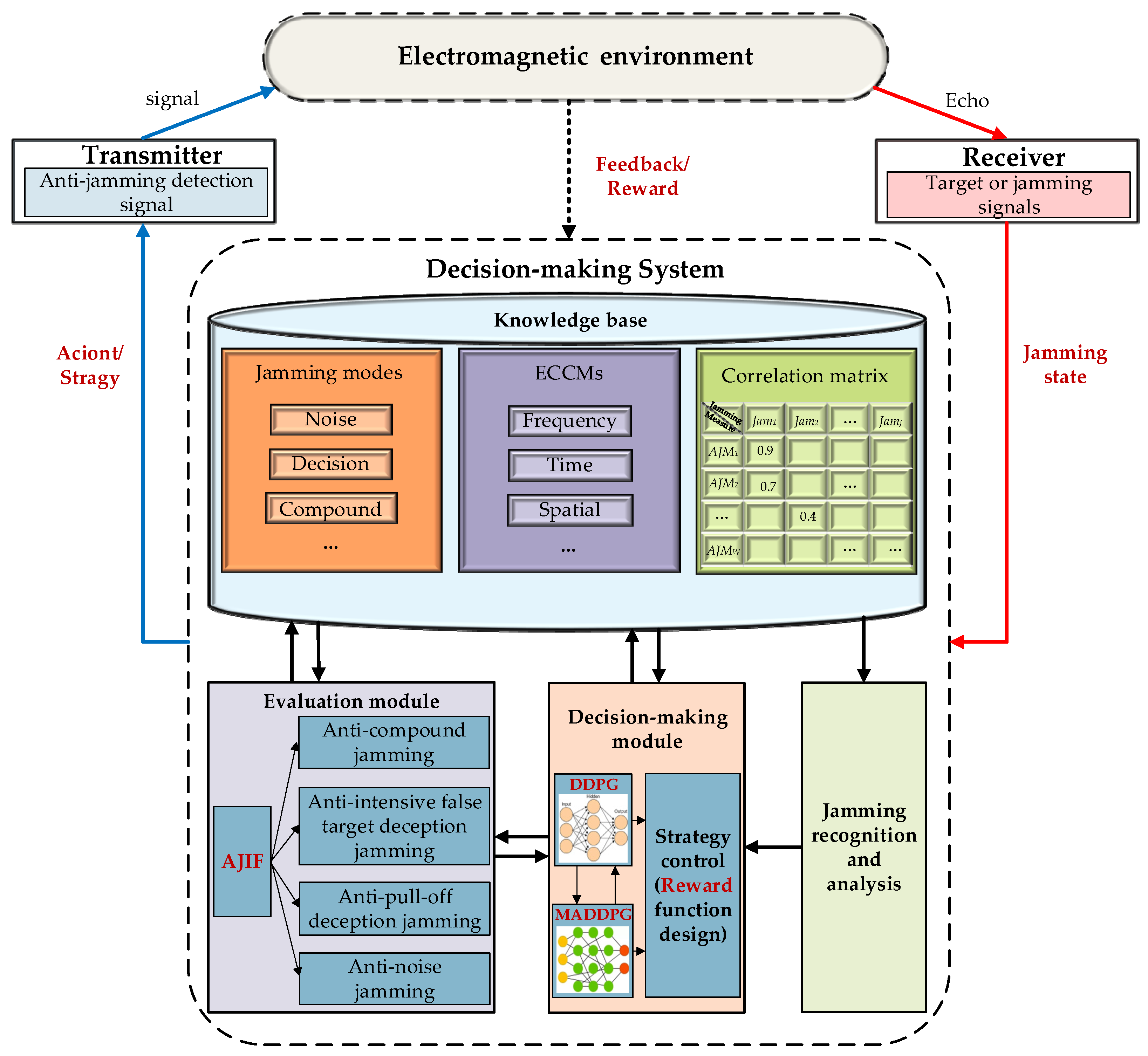
• We established a typical electronic radar and jamming countermeasure scenario and divided various jamming modes and ECCMs according to different categories. Therefore, the dimension of the radar anti-jamming knowledge base was reduced by layering. According to the dynamic interaction process between radar and jamming, we proposed an intelligent radar anti-jamming decision-making model. By defining the anti-jamming decision-making elements of the radar, the radar anti-jamming decision-making process was formulated. This is the basis for the design of the anti-jamming decision-making algorithm.
• An anti-jamming improvement factor was designed to evaluate the performance of ECCMs, which can provide feedback to the decision-making algorithm. Based on the anti-jamming improvement factor, we established the correlation matrix of jamming and ECCM, which provides prior knowledge for the decision-making algorithm. Then, according to the limitation of radar anti-jamming resources, we designed four decisioned objectives and constraints to verify the performance of the anti-jamming decision-making algorithm.
• We designed the DDPG-MADDPG algorithm to generate anti-jamming strategies, which includes the outer DDPG algorithm and the inner MADDPG algorithm. Through the hierarchical selection and joint optimization of two layers, this not only reduces the dimensionality of the action space, but also finds the global optimal solution in a shorter convergence time. Simulation results proved that this method has better robustness, a shorter convergence time, higher decision making accuracy, and better generalization performance.

The rest of this paper is organized as follows: the intelligent radar anti-jamming decision-making model is introduced in Section 2. The radar anti-jamming decision-making method based on the DDPG-MADDPG algorithm is explained in Section 3. Section 4 shows the specifics of the simulations and the analysis of the results, followed by the conclusion presented in Section 5.

2. Materials

2.1. Working Scenario of Radar and Jamming

According to the search and tracking operations by radar, the electronic jammer may adopt different jamming strategies and adaptively change the jamming modes during the game between radar and jamming. The working scenario of radar and jamming is shown in Figure 1. There are two targets with jammers, two support jammer, and one stand-off jammer. During the game process, the jammers generate various jamming modes, such as noise jamming, dense false target jamming, pull-off deception jamming and the ECCMs of the radar are also varied. A radar system needs to efficiently select an optimal anti-jamming strategy (an optimal combination of ECCMs) in the high-dimensional knowledge base to deal with variable jamming modes and to maximize its jamming suppression effect.

For different jamming modes and anti-jamming principles, different ECCMs have been investigated. To establish the vast, high-dimensional, and diverse jamming modes and ECCMs database, we conducted research on the jamming modes and ECCMs, respectively. The aim was to establish a database of jamming modes and ECCMs and to provide prior data for the anti-jamming decision-making algorithm. Therefore, we defined countermeasure elements in the database: jamming modes and radar ECCMs. We divided the jamming modes and ECCMs according to the category.

Table 1. The schematic elements of jamming modes divided according to the category.

Category	Jamming Mode	Number
Noise jamming	Blocking jamming	$Ja{m}_1$
	Aiming jamming	$Ja{m}_2$
	Sweep jamming	$Ja{m}_3$
False target deception jamming	Range false target deception jamming	$Ja{m}_4$
	Sample-and-modulation deception jamming	$Ja{m}_5$
	Intensive false target deception jamming	$Ja{m}_6$
Pull-off deception jamming	Range pull-off jamming	$Ja{m}_7$
	Velocity pull-off jamming	$Ja{m}_8$
	Range–velocity simultaneous pull-off jamming	$Ja{m}_9$
Compound jamming	Noise jamming + false target deception jamming	$Ja{m}_{10}$
	Noise jamming + pull-off deception jamming	$Ja{m}_{11}$
	False target deception jamming + pull-off deception	$Ja{m}_{12}$
	…	$Ja{m}_m$

shows the schematic elements of jamming modes divided according to the category. According to different effects on radar, the jamming modes were divided into four categories, including noise jamming, false target deception jamming, pull-off deception jamming, and compound jamming. Noise jamming includes blocking jamming, aiming jamming, sweep jamming, etc. False target deception jamming includes range false target deception, sample-and-modulation deception, intensive false target deception, etc. Pull-off deception jamming includes range pull-off, velocity pull-off, range–velocity simultaneous pull-off, etc. Compound jamming includes noise jamming + false target deception jamming, noise jamming + pull-off deception jamming, false target deception jamming + pull-off deception jamming, etc. There are $M$ jamming modes, and they are numbered in sequence, defined as $\left\{Ja{m}_1,\cdots ,Ja{m}_m,\cdots ,Ja{m}_M\right\}$, where $m\in \left\{1,2,\cdots ,M\right\}$.

Table 2. The schematic elements of ECCMs of radar divided according to transform domains.

Transform Domain		ECCM
Name	Number	Name	Number
Time domain	$T{D}_1$	Linear filter design	$AJ{M}_1$
		LFM waveform parameter design	$AJ{M}_2$
		…	…
Frequency domain	$T{D}_2$	Carrier frequency fixed mode agility	$AJ{M}_1$
		Carrier frequency random agility	$AJ{M}_2$
		…	$AJ{M}_w$
		…	…
Space domain	$T{D}_3$	Space–time adaptive filtering	$AJ{M}_1$
		Adaptive beamforming	$AJ{M}_2$
		Sidelobe cancellation	$AJ{M}_3$
		…	$AJ{M}_w$
…	$T{D}_n$	…	…

shows the schematic elements of ECCMs divided according to the transform domains. According to the different transform domains, the ECCMs are divided into $N$ domains, which are denoted as $\left\{T{D}_1,\cdots ,T{D}_n,\cdots ,T{D}_N\right\}$, where $n\in \left\{1,2,\cdots ,N\right\}$, such as time domain, frequency domain, space domain, etc. Each transform domain $T{D}_n$ contains $W$ ECCMs, and they are denoted as $\left\{AJ{M}_1,\cdots ,AJ{M}_w,\cdots ,AJ{M}_W\right\}$, where $w\in \left\{1,2,\cdots ,W\right\}$. For example, the time domain includes linear filter design, LFM waveform parameter design, etc. The frequency domain includes carrier frequency fixed mode agility, carrier frequency random agility, etc. The space domain includes space–time adaptive filtering, adaptive beamforming, sidelobe cancellation, etc.

2.2. Intelligent Radar Anti-Jamming Decision-Making Model

In the intelligent game process radar and jamming, the radar observes less information about the complex electromagnetic environment, and the way the radar interacts with jamming determines whether the anti-jamming strategy can successfully suppress jamming. Therefore, the interaction process between radar and jamming is defined as follows: in the first decision-making round, the radar receives a jamming strategy from the electromagnetic environment. According to the decision-making goal, the radar quickly selects the current optimal combination of ECCMs in the high-dimensional and hierarchical knowledge base, after which the anti-jamming strategy is implemented. In the second decision-making round, the radar anti-jamming strategy is optimized according to the anti-jamming effect feedback received from the electromagnetic environment. During one decision-making cycle, this process is repeated continuously. Ultimately, the goal of the radar is to determine the optimal anti-jamming strategy to deal with the jamming strategy. Therefore, an intelligent radar anti-jamming decision-making model is established, as shown in Figure 2. The intelligent radar anti-jamming decision-making model includes four parts: the electromagnetic environment, the receiver, the decision-making system, and the transmitter. Firstly, the echo from the electromagnetic environment is received by the receiver to obtain the target and jamming signals. Then, based on the knowledge base, the observed jamming signal is analyzed, and the anti-jamming strategy is generated by the decision-making system. Finally, the radar communicates with the electromagnetic environment through the transmitter.

The decision-making system includes a knowledge base, a decision-making module, an evaluation module, and a jamming recognition and analysis module. The knowledge base contains the jamming information, ECCMs, and the correlation matrix of jamming modes and ECCMs. The correlation matrix of jamming modes and ECCMs expresses the effect value of ECCMs on suppressing each jamming mode and provides prior information for anti-jamming decision making. The decision-making module optimizes the transform domains and ECCMs to learn anti-jamming strategies online and thereafter updates the knowledge base. The evaluation module is used to evaluate the performance of the ECCMs, and the results are used as the feedback of the decision-making module to update the anti-jamming strategy. The jamming information from the jamming recognition and analysis module is considered already known.

If we consider the radar and the electromagnetic jamming environment as the agent and the environment, then we can model the radar anti-jamming decision-making problem as a Markov decision process (MDP) using RL theory [15]. The anti-jamming decision-making process of the radar can be defined as a tuple $\left\{S,A,P,R\right\}$, where the decision-making elements are shown in

Table 3. The anti-jamming decision-making elements of the radar.

Name	Variable
Agent	Radar
Environment	Electromagnetic jamming environment
State $s_t$	Jamming mode $Ja{m}_m$
Action $a_t$	${\left(a_t\right)}_{layer1}$: transform domains, ${\left(a_t\right)}_{layer2}$: ECCMs.
Reward $r_t$	Anti-jamming evaluation result
The policy $\pi \left(a_t\left|s_t\right.\right)$	The probability that radar chooses ${\left(a_t\right)}_{layer1}$ and ${\left(a_t\right)}_{layer2}$
Decision-making cycle	200 pulse repetition intervals (PRIs)

. $S$ is a finite set of state $s_t$, where $s_t\in S$. The state $s_t$ at time $t$ is defined as jamming mode $Ja{m}_m$, $Ja{m}_m\in \left\{Ja{m}_1,\cdots ,Ja{m}_m,\cdots ,Ja{m}_M\right\}$. $A$ is a finite set of action $a_t$, where $a\in A$. In order to reduce the dimensionality of the action space, the action $a_t$ at time $t$ is the layered ECCMs. We divide action $a_t$ into action layer1 ${\left(a_t\right)}_{layer1}$ and action layer2 ${\left(a_t\right)}_{layer2}$, where ${\left(a_t\right)}_{layer1}\in \left\{T{D}_1,\cdots ,T{D}_n,\cdots ,T{D}_N\right\}$, ${\left(a_t\right)}_{layer2}\in \left\{AJ{M}_1,\cdots ,AJ{M}_w,\cdots ,AJ{M}_W\right\}$. Action layer1 ${\left(a_t\right)}_{layer1}$ contains one or more transform domains, and action layer2 ${\left(a_t\right)}_{layer2}$ also contains one or more ECCMs. Therefore, the radar action is a cascading use of ECCMs in multiple domains. $P\left(s_{t+1}\left|s_t,a_t\right.\right)$ is the transition probability describing how the current state $s_t$ transfers to the next state $s_{t+1}$ when the agent takes action $a_t$.$R$ is a finite set of the immediate reward $r_t$, where $r_t\in R$. We use the anti-jamming evaluation result as a reward $r_t$ to optimize the anti-jamming strategy when the decision-making system takes action $a_t$ according to policy $\pi \left(a_t\left|s_t\right.\right)$ and the state changes from $s_t$ to $s_{t+1}$. The policy $\pi \left(a_t\left|s_t\right.\right)$ is a mapping function of probability distributions from state $s_t$ to action $a_t$.

Therefore, the confrontation process between the radar and the electromagnetic environment can be described as follows. The decision-making system is in state $s_t=Ja{m}_m$ at time $t$ and chooses an action $a_t=\left\{{\left(a_t\right)}_{layer1},{\left(a_t\right)}_{layer2}\right\}$ according to policy $\pi \left(a_t\left|s_t\right.\right)$. When the state is transferred from $s_t=Ja{m}_j$ to $s_{t+1}=Ja{m}_m{}^{\prime }$, the evaluation module of the decision-making system evaluates the anti-jamming effect. The evaluation result is fed back to the decision-making algorithm as the reward $r_t=R$. The objective of the decision-making system is to maximize the long-term expected reward and find the optimal policy ${\pi }^{\ast }$. The optimal policy ${\pi }^{\ast }$ is denoted as

$${\pi }^{\ast }=\arg \underset{\pi }{\max } \mathrm{E}{\displaystyle \left[R_t\left|\pi \right.\right]}$$

(1)

where $R_t={\displaystyle \sum _{k=0}^{\infty }{\gamma }^k{r}_{t+k}}$ represents discounted long-term returns. $\gamma \in \left(0,1\right]$ is the discount factor. $\mathrm{E}\left[R_t\left|\pi \right.\right]$ represents the long-term expected returns.

3. Methods

3.1. Anti-Jamming Improvement Factor and Decision-Making Objectives

3.1.1. Anti-Jamming Improvement Factor

We designed an anti-jamming improvement factor (AJIF) to evaluate the jamming suppression effect of ECCMs and used it as feedback to express the reward function in the anti-jamming decision-making algorithm. AJIF describes the improved anti-jamming capability of the radar with ECCMs compared to without ECCMs. We chose different evaluation indicators, respectively, for four different categories of jamming modes [41], as shown in

Table 4. The evaluation indicators for four different categories of jamming modes.

Jamming Category	Evaluation Indicator
Noise jamming	SINR
False target deception jamming	The number of real targets found
Pull-off deception jamming	Tracking accuracy error
Compound jamming	The mathematical accumulation of evaluation indicators of each single jamming

. When the radar is subjected to noise jamming, lots of noise signals enter the receiver, which reduces the signal-to-noise ratio output by the receiver and reduces the detection probability. If the SINR is larger after anti-jamming measures are taken, it means the effect of the anti-jamming measures is better. Therefore, the anti-jamming evaluation indicator of noise jamming is selected as the SINR. False target deception jamming affects the normal detection performance of the radar by producing a certain number of false targets, causing the radar to lose real targets. When the number of false targets reaches a certain amount, it will suppress the radar. If the radar finds more real targets after taking anti-jamming measures, it means that the effect is better. Therefore, the anti-jamming evaluation indicator of false target deception jamming is selected as the number of real targets found.

Pull-off deception jamming is mainly used to interfere with the automatic tracker of the radar and to lead the tracker of the radar to a wrong position far away from the real target to achieve the effect of exchanging the fake for the real. Therefore, its impact on radar is mainly reflected in the error of tracking accuracy. If the radar tracking accuracy error is smaller after anti-jamming measures are taken, it means that the effect of the anti-jamming measures is better. Therefore, the anti-jamming evaluation indicator of pull-off deception jamming is selected as the tracking accuracy error. Compound jamming can produce the effect of “1 + 1 > 2”, increasing the difficulty of anti-jamming. The combination of multiple jamming signals can increase the ambiguity of the received deceptive jamming signal while reducing the detection probability of the real target echo by the radar. It makes it difficult to distinguish the real target echo from the spoofed jamming echo, which further interferes with the normal operation of the target radar. Therefore, the anti-jamming evaluation indicator of compound jamming is the mathematical accumulation of the evaluation indicators of each single jamming.

Suppose the value of the evaluation indicator when the radar is not jammed is $P_0$, and the value of the evaluation indicator when the radar is jammed is $P_{\mathrm{J}}$. The value of the evaluation indicator after taking ECCM is $P_{\mathrm{AJ}}$, and the AJIF of the $w\mathrm{th}$ ECCM against the $m\mathrm{th}$ jamming is defined as:

$$e_{wm}=\frac{{\left(P_{\mathrm{AJ}}\right)}_{wm}}{{\left(P_0\right)}_{wm}-{\left(P_{\mathrm{J}}\right)}_{wm}}$$

(2)

where $w=1,2,\cdots ,W$, $m=1,2,\cdots ,M$. There are $w$ ECCMs and $m$ jamming modes.

Because different evaluation indicators have different value ranges, we need to normalize AJIF as follows:

$${\overline{e}}_{wm}=\frac{e_{wm}-X_{wm\min }}{X_{wm\max }-X_{wm\min }}$$

(3)

where $X_{wm\min }$ and $X_{wm\max }$ are the minimum and maximum of $e_{wm}$, respectively.

The AJIF vector of the $w\mathrm{th}$ ECCM that suppresses $m\mathrm{th}$ jamming is defined as:

$$E_w={\left({\overline{e}}_{w1},{\overline{e}}_{w2},\cdots ,{\overline{e}}_{wj}\right)}^T$$

(4)

We define a correlation matrix $CM$ of jamming and ECCM, which is a quantitative evaluation result based on AJIF. It is used to describe the relationship between jamming and ECCM and to provide prior knowledge for the decision-making algorithm. The correlation matrix is represented by a two-dimensional matrix $CM$.

$$\begin{array}{l}C{M}_{W\times M}={\left({\overline{e}}_{wm}\right)}_{W\times M}\\ ={\left(E_1,E_2,\cdots ,E_W\right)}_M\end{array}$$

(5)

Because there are $N$ sub-domains, there are $N$ $C{M}_{W\times M}$, which are defined as a matrix: ${\left[{\left(C{M}_{W\times M}\right)}_1,\cdots ,{\left(C{M}_{W\times M}\right)}_n,\cdots ,{\left(C{M}_{W\times M}\right)}_N\right]}^T$.

3.1.2. Decision-Making Objectives and Constraints

The AJIF ${\overline{e}}_{wm}$ can be used as an immediate reward $r_t$ to provide feedback to the decision-making algorithm. However, within one decision cycle, the optimization of ECCMs needs to be based on the decision-making objectives of the radar. Therefore, according to the actual task requirements in the radar combat process, we designed four decision-making objectives ranging from simple to complex.

For situations in which only the jamming suppression effect of ECCMs is considered, we designed decision-making objective 1. In order to make the best anti-jamming effect, the accumulated sum of AJIF ${\overline{e}}_{wm}$ of all selected ECCMs should be maximized. Decision-making objective 1 $Rewar{d}_1$ is as follows:

$$Rewar{d}_1=\max {\displaystyle \sum _{n=1}^N{\overline{e}}_{wm}}$$

(6)

In order to make the difference in the jamming suppression effect values between the selected ECCMs small, we chose the average value of the jamming suppression effect as the decision-making objective 2 and maximized the average value of the accumulated sum of AJIF ${\overline{e}}_{wm}$ of all selected ECCMs. Decision-making objective 2 $Rewar{d}_2$ is as follows:

$$Rewar{d}_2=\frac{1}{N}{\displaystyle \sum _{n=1}^N{\overline{e}}_{wm}}$$

(7)

In the decision-making process, the more ECCMs are selected, the more anti-jamming resources are occupied. In decision-making objectives 1 and 2, although the jamming suppression performance is improved, it is not conducive to saving resources. Therefore, we employed a weighted approach that maximizes the cumulative sum of the AJIF ${\overline{e}}_{wm}$ while minimizing the number of selected ECCMs. When the two sub-goals are equally important, decision-making objective 3 is defined as:

$$Rewar{d}_3=\frac{0.5\times {\alpha }_1}{\max {\displaystyle \sum _{n=1}^N{e}_{wm}}}\times {\displaystyle \sum _{n=1}^N{e}_{wm}}-\frac{0.5\times {\alpha }_2}{N}\times n$$

(8)

where ${\gamma }_1$ and ${\gamma }_2$ are the importance weight, ${\gamma }_1=0.5$, ${\gamma }_2=0.5$, ${\gamma }_1+{\gamma }_2=1$. ${\alpha }_1$ and ${\alpha }_2$ are the empirical coefficients, determined according to expert experience.

When the suppression effect is more important, the weights of the two objectives are designed to be ${\gamma }_1=0.87$ and ${\gamma }_2=0.13$, respectively. Decision-making objective 4 is defined as:

$$Rewar{d}_4=\frac{0.8\times {\alpha }_1}{\max {\displaystyle \sum _{n=1}^N{e}_{wm}}}\times {\displaystyle \sum _{n=1}^N{e}_{wm}}-\frac{0.2\times {\alpha }_2}{N}\times n$$

(9)

In the anti-jamming process, the ECCMs in some sub-domains cannot be used at the same time. For example, the inter-pulse frequency-agile waveform in the frequency sub-domain cannot be used at the same time as the LFM signal ECCM in the waveform sub-domain. Therefore, we set constraints and a prior knowledge base $KB$. The transform sub-domains $\left\{T{D}_1,\cdots ,T{D}_n,\cdots ,T{D}_N\right\}$ are encoded from 1 to $N$, and the transform sub-domains are permutated and combined to generate $V$ combinations $V{C}_v$, $v\in \left\{1,2,\cdots ,V\right\},V=C_N^1+C_N^2+\cdots C_N^n+\cdots +C_N^N$. We pre-select the combinations of transform sub-domains where ECCMs cannot be cascaded through expert knowledge. They are put into the prior knowledge base $KB$ and named $constrans\_V{C}_v$. The constraint condition of the decision-making algorithm is to judge whether the action exists in the knowledge base $KB$.

3.2. Anti-Jamming Decision-Making Algorithm Based on DDPG-MADDPG

3.2.1. Preliminaries

The DDPG algorithm is an online DRL algorithm under the actor–critic framework [42]. It includes an actor network and a critical network, each of which follows its own update law to maximize the cumulative expected return. In order to solve the optimal policy ${\pi }^{\ast }$ from Section 2.2, we make $\mu =\pi \left(a_t\left|s_t\right.\right)$. If the target policy is $\mu :\mathcal{S}\leftarrow \mathcal{A}$, the critic network uses the Bellman equation to express the optimal action value function [43] as follows:

$$Q^{\mu }\left(s_t,a_t\right)={\mathbb{E}}_{r_t,s_{t+1}\sim E}\left[r\left(s_t,a_t\right)+\gamma Q^{\mu }\left(s_{t+1},\mu \left(s_{t+1}\right)\right)\right]$$

(10)

$Q^{\mu }\left(s_t,a_t\right)$ depends on the environment, and it is possible to learn the $Q^{\mu }$ off-policy by using transitions generated via the different stochastic behavior policy $\beta$. By minimizing the loss between the Q-function and the target value [44], the critic network ${\theta }^Q$ is optimized:

$$L\left({\theta }^Q\right)={\mathbb{E}}_{s_t\sim {\rho }^{\beta },a_t\sim \beta ,r_t\sim E}\left[{\left(Q\left(s_t,a_t\mid {\theta }^Q\right)-y_t\right)}^2\right]$$

(11)

where ${\theta }^Q$ denotes the parameters of policy $\beta$. The target value $y_t$ is obtained by:

$$y_t=r\left(s_t,a_t\right)+\gamma Q\left(s_{t+1},\mu \left(s_{t+1}\right)\mid {\theta }^Q\right)$$

(12)

DDPG keeps a parameterized actor function $\mu \left(s\left|{\theta }^{\mu }\right.\right)$ that defines the current policy by deterministically mapping states to precise actions. The critic function $Q\left(s,a\right)$ is learned using the Bellman equation. By applying the chain rule on the expected return from the start distribution $J$ with the actor parameters, the actor network is updated:

$$\begin{array}{ll}\hfill {\nabla }_{{\theta }^{\mu }}J& \approx {\mathbb{E}}_{s_t\sim {\rho }^{\beta }}\left[{\nabla }_{{\theta }^{\mu }}Q\left(s,a\left|{\theta }^Q\right.\right)\left|{}_{s=s_t,a=\mu \left(s_t\left|{\theta }^{\mu }\right.\right)}\right.\right]\hfill \\ & \approx {\mathbb{E}}_{s_t\sim {\rho }^{\beta }}\left[{\nabla }_{a}Q\left(s,a\left|{\theta }^Q\right.\right)\left|{}_{s=s_t,a=\mu \left(s_t\right)}\right.{\nabla }_{{\theta }^{\mu }}\mu \left(s\left|{\theta }^Q\right.\right)\left|{}_{s=s_t}\right.\right]\hfill \end{array}$$

(13)

DDPG uses a replay buffer to address the issue that the samples are independent and identically distributed. The replay buffer is a finite-sized cache $\mathcal{D}$. Transitions are sampled from the environment according to the exploration policy and the tuple $\left(s_t,a_t,r_t,s_{t+1}\right)$ is stored in the replay buffer. It constructs an exploration policy ${\mu }^{\prime }$ by adding noise sampled from a noise process $\mathcal{N}$ to our actor policy:

$${\mu }^{\prime }\left(s_t\right)=\mu \left(s_t\left|{\theta }_t^{\mu }\right.\right)+\mathcal{N}$$

(14)

MADDPG can enable multiple sub-agents to complete intricate tasks through communication interaction and collaborative decision making in a high-dimensional and dynamic environment [45]. Consider a game with $N$ sub-agents and continuous policies ${\mathsf{\mu }}_{{\theta }_n}$ (abbreviated as ${\mathsf{\mu }}_{{\theta }_n}$) that is parameterized by $\mathsf{\theta }=\left\{{\theta }_1,\dots ,{\theta }_N\right\}$ for more detail. The gradient $J\left({\mu }_n\right)=\mathbb{E}\left[R_n\right]$ of the anticipated return for the sub-agent $n$ can be expressed as:

$${\nabla }_{{\theta }_n}J\left({\mathsf{\mu }}_n\right)={\mathbb{E}}_{x,a\sim \mathcal{D}}\left[{\nabla }_{{\theta }_n}{\mathsf{\mu }}_n\left(a_n\mid o_n\right){\nabla }_{a_n}{Q}_n^{\mathsf{\mu }}\left(\mathrm{x},a_1,\dots ,a_N\right)\left|{}_{a_n={\mathsf{\mu }}_n\left(o_n\right)}\right.\right]$$

(15)

where the $Q_n^{\mu }\left(x,a_1,\dots ,a_N\right)$ is a centralized action-value function that outputs the Q-value for the sub-agent $n$ after receiving the collective actions of all sub-agents, $a_1,\dots ,a_N$, and some state data $x$, as inputs. In its most basic form, $x$ might be made up of all sub-agents’ observations, $X=\left(O_1,\dots ,O_N\right)$. The sub-agent $n$ obtains a personal observation $O_n$ connected with the state. The tuples $\left(\mathrm{x}, {\mathrm{x}}^{\prime }, a_1,\dots ,a_N, r_1,\dots ,r_N\right)$, which record the experiences of all sub-agents, are contained in the experience replay buffer $\mathcal{D}$.

The action-value function $Q_n^{\mu }$ is updated as:

$$\mathcal{L}\left({\theta }_n\right)={\mathbb{E}}_{x,a,r,x^{\prime }}\left[{\left(Q_n^{\mathsf{\mu }}\left(x,a_1,\dots ,a_N\right)-y\right)}^2\right],y=r_n+\gamma Q_n^{{\mathsf{\mu }}^{\prime }}\left({\mathrm{x}}^{\prime },a_1^{\prime },\dots ,a_N^{\prime }\right)\left|{}_{a_j^{\prime }={\mathsf{\mu }}_j^{\prime }\left(o_j\right)}\right.$$

(16)

where ${\mathsf{\mu }}^{\prime }=\left\{{\mathsf{\mu }}_{{\theta }_1^{\prime }},\dots ,{\mathsf{\mu }}_{{\theta }_N^{\prime }}\right\}$ is one of the target policies in the collection with the delayed parameters ${\theta }_n^{\prime }$.

Each sub-agent $n$ can furthermore retain an approximation ${\widehat{\mu }}_{{\varphi }_n^j}$ (where $\varphi$ are the parameters of the approximation; hereafter ${\widehat{\mu }}_n^j$) to the genuine policy of sub-agent $j$, ${\mu }_j$, eliminating the premise of knowing other sub-agents’ policies, as required by (16). By maximizing the log-likelihood of sub-agent $j\prime s$ actions and using an entropy regularizer, this approximation of a policy is learned by:

$$\mathcal{L}\left({\varphi }_n^j\right)=-{\mathbb{E}}_{o_j,a_j}\left[\log {\widehat{\mathsf{\mu }}}_n^j\left(a_j\mid o_j\right)+\lambda H\left({\widehat{\mathsf{\mu }}}_n^j\right)\right]$$

(17)

where $H$ is the policy distribution’s entropy. With the approximation policies, the value $y$ in (16) can be roughly computed as follows:

$$\widehat{y}=r_n+\gamma Q_n^{{\mu }^{\prime }}\left(x^{\prime },{\widehat{\mu }}_n^{\prime 1}\left(o_1\right),\dots ,{\mu }_n^{\prime }\left(o_n\right),\dots ,{\widehat{\mu }}_n^{\prime N}\left(o_N\right)\right)$$

(18)

where the approximate policy ${\widehat{\mu }}_n^j$’s target network is denoted by the letter ${{\widehat{\mu }}^{\prime }}_n^j$. It should be noted that (17) can be optimized entirely online: we extract the most recent samples of each sub-agent $j$ from the replay buffer to update $Q_n^{\mu }$, the centralized Q function, in a single gradient step before updating ${\varphi }_n^j$.

To produce multi-agent policies that are more resistant to changes in competing sub-agents’ policies, it trains a collection of $K$ different sub-policies. Each episode, it chooses one sub-policy at random for each sub-agent to carry out. Assume that policy ${\mu }_n$ is an ensemble of $K$ various sub-policies, with sub-policy $k$ denoted by ${\mathsf{\mu }}_{{\theta }_n^{(k)}}$ (denoted as ${\mathsf{\mu }}_n^{\left(k\right)}$). The ensemble objective is maximized for sub-agent $n$: $J_e\left({\mathsf{\mu }}_n\right)={\mathbb{E}}_{k\sim unif(1,K),s\sim p^{\mu },a\sim {\mathsf{\mu }}_n^{(k)}}\left[R_n(s,a)\right]$. Because various sub-policies will be executed in separate episodes, we keep a replay buffer ${\mathcal{D}}_n^{\left(k\right)}$ for each sub-policy ${\mathsf{\mu }}_n^{\left(k\right)}$ of sub-agent $n$. As a result, the gradient of the ensemble goal with respect to ${\theta }_n^{\left(k\right)}$ may be calculated as follows:

$${\nabla }_{{\theta }_n^{\left(k\right)}}{J}_e\left({\mathsf{\mu }}_n\right)=\frac{1}{K}{\mathbb{E}}_{x,a\sim {\mathcal{D}}_n^{\left(k\right)}}\left[{\nabla }_{{\theta }_n^{\left(k\right)}}{\mathsf{\mu }}_n^{\left(k\right)}\left(a_n\mid o_n\right){\nabla }_{a_n}{Q}_n^{{\mathsf{\mu }}_n}\left(\mathrm{x},a_1,\dots ,a_N\right)\left|{}_{a_n={\mathsf{\mu }}_n^{\left(k\right)}\left(o_n\right)}\right.\right]$$

(19)

3.2.2. DDPG-MADDPG Algorithm

In order to cope with varied jamming modes, it is necessary to solve the problem of efficiently optimizing ECCMs in a high-dimensional and layered knowledge base. Therefore, we propose a dual RL model based on the DDPG-MADDPG algorithm. It comprises an outer DDPG and an inner MADDPG, as shown in Figure 3. To reduce the dimensionality of the action space, we divide the radar action space into two sub-spaces containing the transform domain and the ECCM. The anti-jamming process is divided into two layers. The first decision-making layer is the outer DDPG, which uses the DDPG algorithm to select the transform sub-domains. The second decision-making layer is the inner MADDPG, which uses the MADDPG algorithm to select ECCMs according to the transform sub-domains. We found the global optimal solution by interacting the outer DDPG with the inner MADDPG. The interaction between the two layers can be described as follows: the outer DDPG determines the transform sub-domains and guides the actions of the inner MADDPG. The ECCMs determined by the inner MADDPG directly determine the anti-jamming effect of the radar and affect the choice of the next decision-making action.

The outer DDPG contains the agent 1. The observation state is defined by the jamming modes. The state $s_t^1$ at time $t$ is an $M$-dimensional vector encoded by 1 and 0, with each dimension corresponding to one jamming mode. The dimension of vector $s_t^1$ with jamming is set to 1 and the dimension of vector $s_t^1$ without jamming is set to 0. For example, if $M=8,m=3$, there is $s_t^1=\left[0,0,1,0,0,0,0,0\right]$. The output action is defined by transform domains. We encode all combinations $V{C}_v$ sequentially from 1 to $V$. The action $a_t^1$ at time $t$ is an eight-bit binary code of combinations $V{C}_v$. For example, if $N=4,V=15,v=3$, there is $a_t^1=\left[0,0,0,0,0,0,1,1\right]$. We set decision-making constraints. When the action of agent1 selected exists in the $KB$, then $rewar{d}^1=-\infty$. Otherwise, go to the next step. The feedback reward is defined by decision-making objectives. Because there are four decision-making objectives, we define four rewards, $rewar{d}_1^1=Rewar{d}_1,rewar{d}_2^1=Rewar{d}_2,rewar{d}_3^1=Rewar{d}_3,rewar{d}_4^1=Rewar{d}_4$, to optimize the DDPG-MADDPG model, respectively. The $Q^1\left(s^1,a^1\mid {\theta }^{Q^1}\right)$ and $Q^{1\prime }\left(s^1,a^1\mid {\theta }^{Q^{1\prime }}\right)$ of the critic network are optimized by Equation (10). The ${\theta }^{Q^1}$ and ${\theta }^{Q^{1\prime }}$ of the critic network are optimized by Equation (11). The ${\mu }^1\left(s^1\mid {\theta }^{{\mu }^1}\right)$ and ${\mu }^{1\prime }\left(s^1\mid {\theta }^{{\mu }^{1\prime }}\right)$ of the actor network are optimized by Equation (14). The ${\theta }^{{\mu }^1}$ and ${\theta }^{{\mu }^{1\prime }}$ of the actor network are optimized by Equation (13).

For the inner MADDPG, we regard $N$ transform domains as $N$ sub-agents, and $w$ ECCMs as the sub-agent’s $w$-dimensional action space. Each sub-agent contains a $w$-dimensional action space. We define the state, action, and reward of the $n\mathrm{th}$ sub-agent as follows. The observation state is defined by the transform sub-domains and the jamming modes. The state $o_n^2$ at time $t$ is an $M+8$-dimensional vector by combining the vector $a_t^1$ and the vector $s_t^1$, where $o_n^2=\left[a_t^1,s_t^1\right]$. For example, if $M=8, m=3, N=4, V=15, v=3$, there is $o_n^2=\left[0,0,0,0,0,0,1,1,0,0,1,0,0,0,0,0\right]$. The output action is defined by ECCMs $\left\{AJ{M}_1,\cdots ,AJ{M}_w,\cdots ,AJ{M}_W\right\}$. The action $A_n^{a_t^2}$ at time $t$ is a $W$-dimensional vector encoded by 1 and 0, with each dimension corresponding to one ECCM. The dimension of the vector $A_n^{a_t^2}$ with the selected ECCM is 1, and the dimension of the vector $A_n^{a_t^2}$ without the selected ECCM is 0. For example, if $W=4, w=2$, there is $A_n^{a_t^2}=\left[0,1,0,0\right]$. The coordinated decisions of multiple transform sub-domains fully cooperate. The goal of each sub-agent in complete cooperation is to maximize the common reward. Therefore, the reward function of all sub-agents is the same. Therefore, the feedback reward is defined by AJIF ${\overline{e}}_{wm}$, where $rewar{d}_n^2={\overline{e}}_{wm}$. The decision goal of each sub-agent is to find the action with the highest AJIF ${\overline{e}}_{wm}$ value in the sub-action space within a decision-making period. The rewards $rewar{d}^2$ of all sub-agents are fed back to DDPG for its optimization strategy. The network optimization method of each sub-agent is the same as that of DDPG.

In order to improve the operating efficiency of the algorithm, we adopted a centralized training distributed execution framework in MADDPG. It solves the problem of network parameter explosion caused by independent training execution of the actor–critic network for each sub-agent. During the training and testing process of the DDPG-MADDPG algorithm, we adopted the method of simultaneous optimization of the outer DDPG and inner MADDPG. Compared with sequential optimization, it not only reduces the dimensionality of the action space, but also finds the global optimal solution in a shorter convergence time. We used the Gumbel Softmax trick to solve the problem that the algorithm cannot handle discrete action spaces [46]. The sampling of the output distribution of the policy network in the algorithm is converted into calculating a fixed learnable probability plus a noise independent of the policy network. In particular, we reconstructed the discrete action space sampling process of DDPG and MADDPG as continuous. This enables the policy network to be efficiently optimized via gradient descent, and, finally, to output discrete actions.

The algorithm of the radar anti-jamming decision-making training algorithm based on DDPG-MADDPG is shown in Algorithm 1, where the input is the jamming strategy and the output is the anti-jamming strategy.

Algorithm 1: DDPG-MADDPG algorithm.

Initialize parameters.  Initialize replay buffer ${\mathcal{D}}^1$ and ${\mathcal{D}}^2$.  For $\mathrm{episode}=1$ to sample length do:   Initialize a random process ${\mathcal{N}}^1$ and ${\mathcal{N}}^2$ with Gumbel Softmax distribution.   Receive initial state $s_1^1$, $S^{s_1^2}$.   For $t=1$ (DDPG) to the decision-making cycle $dp$ do: Sample action $a_t^1$ from Gumbel Softmax distribution according to the current policy ${\mu }^1\left(s_t\mid {\theta }^{{\mu }^1}\right)$ and exploration noise ${\mathcal{N}}_t^1$. Determine whether $a_t^1$ is in $KB$; if so, set $rewar{d}^1=-\infty$, and return to the previous step. Otherwise, go to the next step.   Execute actions $a_t^1=\left(a_1^1,\dots ,a_N^1\right)$ and observe reward $r_t^1$ and observe new state $s_{t+1}^1$.   Store transition $\left(s_t^1,a_t^1,r_t^1,s_{t+1}^1\right)$ in replay buffer ${\mathcal{D}}^1$.   Sample a random minibatch of $X$ transitions $\left(s_i^1,a_i^1,r_i^1,s_{i+1}^1\right)$ from ${\mathcal{D}}^1$.   Set $y_i^1=r_i^1+\gamma Q^{1\prime }\left(s_{i+1}^1,{\mu }^{1\prime }\left(s_{i+1}^1\left|{\theta }^{{\mu }^{1\prime }}\right.\right)\left|{\theta }^{Q^{1\prime }}\right.\right)$.   Update critic by minimizing the loss: ${\mathcal{L}}^1=\frac{1}{X}{\displaystyle \sum {}_i{\left(y_i^1-Q^1\left(s_i^1,a_i^1\left|{\theta }^{Q^1}\right.\right)\right)}^2}$.   Update the actor policy using the sampled policy gradient:   ${\nabla }_{{\theta }^{{\mu }^1}}J\approx \frac{1}{X}{\displaystyle \sum }_i{\nabla }_{a^1}Q\left(s^1,a^1\left|{\theta }^{Q^1}\right.\right)\left|{}_{s^1=s_i^1,a^1={\mu }^1\left(s_i^1\right)}{\nabla }_{{\theta }^{{\mu }^1}}{\mu }^1\left(s^1\left|{\theta }^{{\mu }^1}\right.\right)\right.\left|s_i^1\right.$.   Update target network parameters:   ${\theta }^{Q^{1\prime }}\leftarrow \tau {\theta }^{Q^1}+(1-\tau ){\theta }^{Q^{1\prime }}$, ${\theta }^{{\mu }^{1\prime }}\leftarrow \tau {\theta }^{{\mu }^1}+(1-\tau ){\theta }^{{\mu }^{1\prime }}$.   End for   for $t=1$ (MADDPG) to sample length do:    for each sub-agent $n$, sample action $A_n^{a_t^2}$ from Gumbel Softmax distribution according to the current policy ${\mu }_n^2\left(s_t^2\mid {\theta }_n^{{\mu }_n^2}\right)$ and exploration noise ${\mathcal{N}}_t^2$.    Execute actions $A^{a_t^2}=\left(A_1^{a_t^2},A_2^{a_t^2},\dots ,A_N^{a_t^2}\right)$ and observe reward $R^{r_t^2}$ and new state $S^{s_{t+1}^2}$.    Store transition $\left(S^{s_t^2},A^{a_t^2},R^{r_t^2},S^{s_{t+1}^2}\right)$ in replay buffer ${\mathcal{D}}^2$.    $S^{s_t^2}\leftarrow S^{s_{t+1}^2}$    for sub-agent $n=1$ to $N$ do     Sample a minibatch of $X$ samples $\left({\left(S^{s_t^2}\right)}^j,{\left(A^{a_t^2}\right)}^j,{\left(R^{r_t^2}\right)}^j,{\left(S^{s_{t+1}^2}\right)}^j\right)$ from ${\mathcal{D}}^2$.     Set $Y^j={\left(R_n^{r_t^2}\right)}^j+\gamma Q_n^{{\mu }^{2\prime }}\left({\left(S^{s_{t+1}^2}\right)}^j,A_1^{a_{t+1}^2},A_2^{a_{t+1}^2},\dots ,A_N^{a_{t+1}^2}\right)\left|{}_{A_k^{a_{t+1}^2}={\mu }_k^{2\prime }\left({\left(o^2\right)}_k^j\right)}\right.$.     Update critic by minimizing the loss:     $\mathcal{L}\left({\theta }_n^{{\mu }^2}\right)=\frac{1}{X}{\displaystyle \sum {}_j{\left(Y^j-Q_n^{{\mu }^2}\left({\left(S^{s_t^2}\right)}^j,{\left(A_1^{a_t^2}\right)}^j,{\left(A_2^{a_t^2}\right)}^j,\dots ,{\left(A_N^{a_t^2}\right)}^j\right)\right)}^2}$.     Update actor using the sampled policy gradient: ${\nabla }_{{\theta }_n^{{\mu }^2}}J\approx \frac{1}{X}{\displaystyle \sum }_j{\nabla }_{{\theta }_n^{{\mu }^2}}{\mu }_n^2\left(o_n^{2j}\right){\nabla }_{a_i^2}{Q}_i^{{\mu }^2}\left({\left(S^{s_t^2}\right)}^j,{\left(A_1^{a_t^2}\right)}^j,\dots ,{\left(A_n^{a_t^2}\right)}^j,\dots ,{\left(A_N^{a_t^2}\right)}^j\right)\left|{}_{{\left(A_n^{a_t^2}\right)}^j={\mu }_n^2\left({\left(o_n^2\right)}^j\right)}\right.$.     End for     Update target network parameters for each sub-agent $b$: ${\theta }_n^{{\mu }^2\prime }\leftarrow \tau {\theta }_n^{{\mu }^2}+(1-\tau ){\theta }_n^{{\mu }^2\prime }$.   end for end for

4. Results

To verify the training effect of the radar anti-jamming decision-making method based on the DDPG-MADDPG algorithm, it is compared with the anti-jamming decision-making method based on the DQN-MADQN algorithm [47] and random decision-making algorithm [40]. The structure of the DQN-MADQN algorithm is the same as that of the DDPG-MADDPG algorithm. DQN optimizes and controls the selection of transform sub-domains, and MADQN optimizes and controls the selection of ECCMs. The random decision algorithm is also divided into two layers. It uses uniform random distribution to select transform sub-domains and ECCMs. Simulation experiments include robust performance verification based on loss function, convergence performance verification based on reward function, decision accuracy verification based on SMAPE, and generalization performance verification based on large action space. The simulation parameters are shown in

Table 5. Simulation parameters.

Parameter	Value
Jamming modes $M$	8
Transform sub-domains $N$	4
ECCMs $W$	4
The number of combinations $V$	15
The number of $constrans\_V{C}_v$ in $KB$	4
Decision-making cycle $dp$	200
Discount factor $\gamma$	0.9
Learning rate of the critic network	0.002
Learning rate of the actor network	0.001
Replay buffer ${\mathcal{D}}^1$ and ${\mathcal{D}}^2$	2048
$X$ samples in one minibatch	64
Sample length	1024
Training time (the number of minibatches)	200

.

Based on expert knowledge and simulation experiments, we obtained the correlation matrix. The schematic elements of the correlation matrix are shown in

Table 6. The schematic elements of the correlation matrix.

Transform Domain	ECCM	Jamming Mode
		$Ja{m}_1$	$Ja{m}_2$	$Ja{m}_3$	$Ja{m}_4$	$Ja{m}_5$	$Ja{m}_6$	$Ja{m}_7$	$Ja{m}_8$	…
$T{D}_1$	$AJ{M}_1$	0.99	0.6	0.99	0.3	0.2	0.3	0.92	0.5	…
	$AJ{M}_2$	0.9	0.5	0.97	0.2	0.1	0.2	0.9	0.4	…
	$AJ{M}_3$	0.1	0.11	0.1	0.65	0.85	0.9	0.3	0.6	…
	$AJ{M}_4$	0.1	0.07	0.12	0.6	0.75	0.8	0.2	0.55	…
	…	…	…	…	…	…	…	…	…	…
$T{D}_2$	$AJ{M}_1$	0	0.01	0.1	0.7	0.6	0.88	0.89	0.7	…
	$AJ{M}_2$	0	0	0.05	0.73	0.65	0.8	0.81	0.73	…
	$AJ{M}_3$	0.1	0.03	0.15	0.9	0.7	0.95	0.96	0.91	…
	$AJ{M}_4$	0	0.01	0.17	0.95	0.73	0.87	0.88	0.96	…
	…	…	…	…	…	…	…	…	…	…
$T{D}_3$	$AJ{M}_1$	0.5	0.6	0.8	0.6	0.97	0	0.5	0.65	…
	$AJ{M}_2$	0.6	0.7	0.95	0.55	0.1	0	0.6	0.6	…
	$AJ{M}_3$	0.6	0.99	0.8	0	0	0	0.3	0.1	…
	$AJ{M}_4$	0.55	0.99	0.77	0	0	0	0.32	0.05	…
	…	…	…	…	…	…	…	…	…	…
$T{D}_4$	$AJ{M}_1$	0	0.1	0.1	0.4	0.2	0.5	0.75	0.82	…
	$AJ{M}_2$	0	0.05	0.2	0.15	0.2	0.6	0.8	0.8	…
	$AJ{M}_3$	0.1	0.13	0.2	0.3	0.45	0.6	0.7	0.4	…
	$AJ{M}_4$	0.15	0.18	0.2	0.35	0.5	0.7	0.8	0.35	…
	…	…	…	…	…	…	…	…	…	…
…	…	…	…	…	…	…	…	…	…	…

. The jamming modes $Ja{m}_1,Ja{m}_2,Ja{m}_3,Ja{m}_4,Ja{m}_5,Ja{m}_6,Ja{m}_7,Ja{m}_8,\cdots$ are denoted as sweep jamming, blocking jamming, aiming jamming, intensive false target jamming, sample-and- modulation deception, range deception jamming, sweep + range deception compound jamming, smart + intensive false target compound jamming, etc. The transform sub-domain is denoted as $T{D}_1,T{D}_2,T{D}_3,T{D}_4,\cdots$, which is denoted as frequency, waveform, spatial and signal processing, etc. The frequency sub-domain $T{D}_1$ includes the inter-pulse frequency-agile waveform $AJ{M}_1$, the intra-pulse sub-frequency-agile waveform $AJ{M}_2$, etc. The waveform sub-domain $T{D}_2$ includes the LFM signal ECCM based on frequency modulation disturbance $AJ{M}_1$, the ECCM based on phase encoding signal $AJ{M}_3$, the ECCM based on frequency-agile signals $AJ{M}_4$, etc.

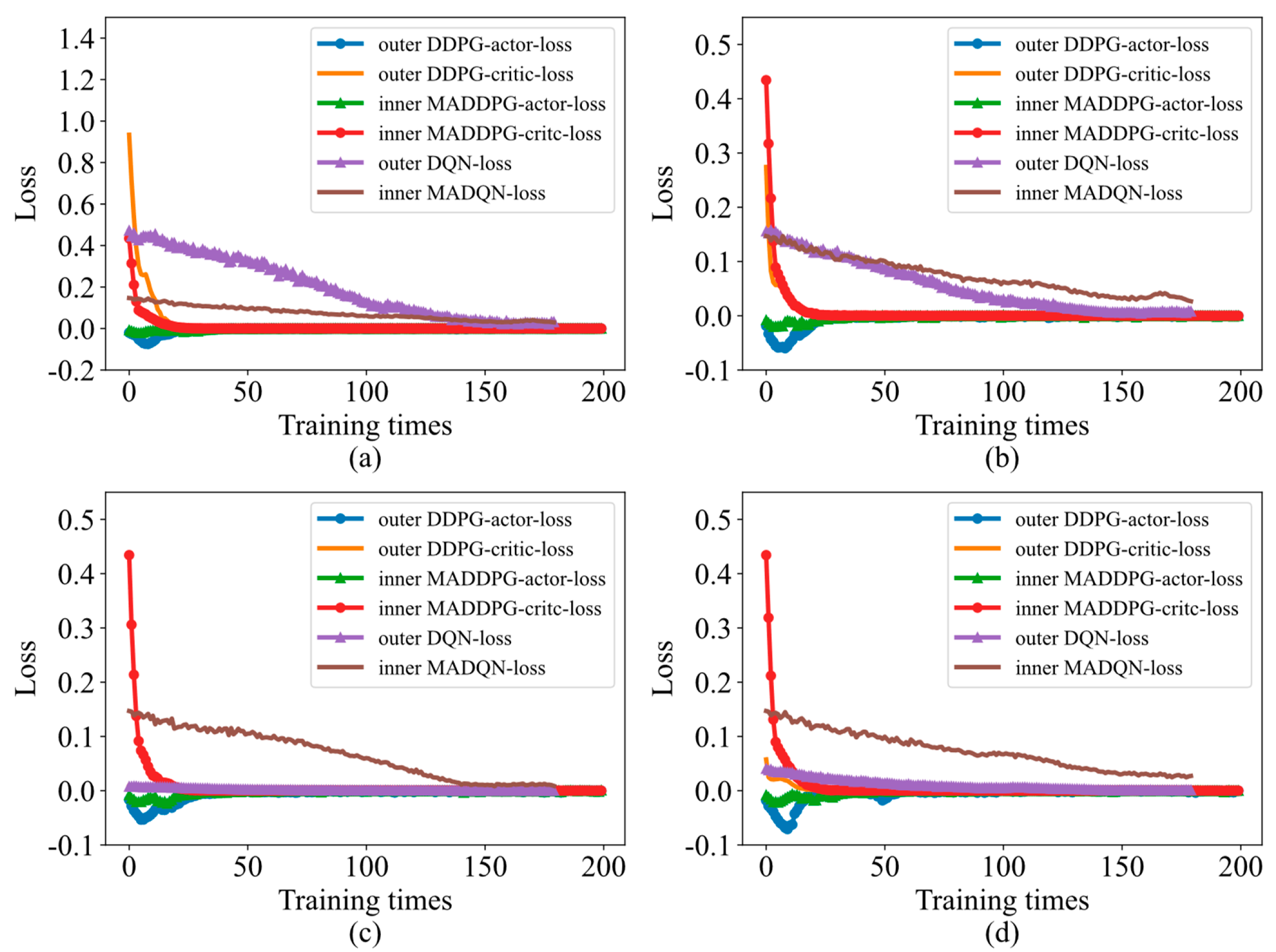
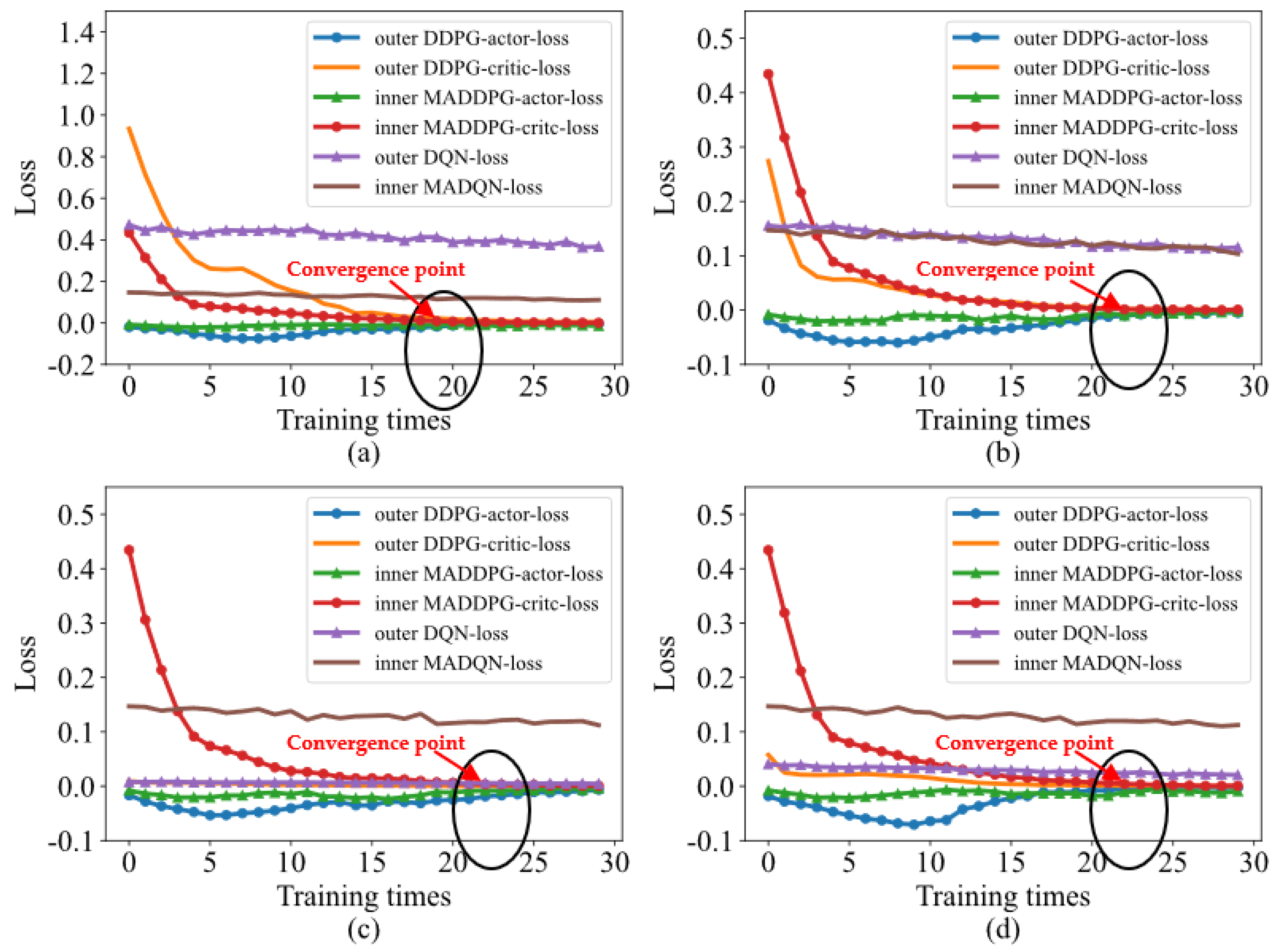
4.1. Robust Performance Based on the Loss Function

In the training process of DRL, the loss function is used to update the learning parameters of the deep neural network (DNN). If the loss function value gradually tends toward 0, it means that the robustness of the algorithm model is better. Therefore, for four decision-making objectives, we analyze the loss function of the neural network. The curve of loss changing with the training times is shown in Figure 4. The loss values of the actor network of outer DDPG and the actor network of inner MADDPG are negative and gradually tend toward 0. This is due to the updating of the actor network using the sampled policy gradient. The update of other neural networks uses cross-entropy loss, so the loss value is positive and tends to become smaller and smaller.

To further explore the convergence speed of the model, we observed the change of loss when the training times were 1–30, as shown in Figure 5. In the case of decision-making objective 1, the neural networks loss value of the DDPG-MADDPG algorithm will all converge to 0 after 19 training times. In the case of decision-making objectives 2, 3, and 4, the neural networks loss values of the DDPG-MADDPG algorithm all converge to 0 after 22 training times. However, in the case of decision-making objectives 1, 2 and 4, the neural networks loss values of the DQN-MADQN algorithm will converge, but none of them can converge to 0. In the case of decision target 3, the neural networks loss values of the outer DQN can converge to 0 at the beginning. The neural networks loss values of the inner MADQN will gradually converge, but they cannot converge to 0. Therefore, the model of the DQN-MADQN algorithm is unstable for different decision-making objectives. In conclusion, through comparison with the DQN-MADQN model, the loss value of the DDPG-MADDPG model can be restrained to 0 in the first 22 training times.

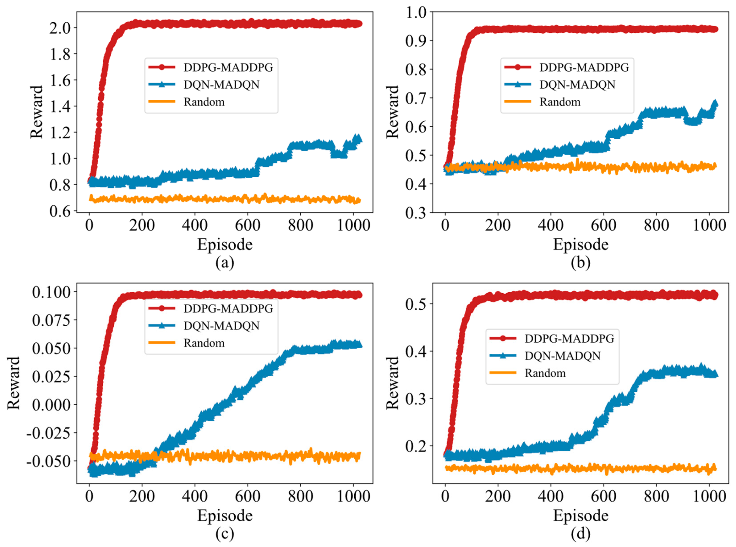
4.2. Convergence Performance Based on Reward Function

To verify the convergence performance of the algorithms, we analyzed the average reward in 1024 decision-making periods, and the curves are shown in Figure 6. In 0–150 episodes, the reward started from 0 and gradually increased. There are two main reasons. One is that in the initial stage, the algorithm is constantly adapting to the environment, which leads to trial and error in the algorithm to find a better anti-jamming strategy. Second, because the algorithm is in the exploratory stage, the weight parameters of the neural network have not reached the optimum, resulting in large fluctuations in the reward value. After 150 episodes, the reward of the DDPG-MADDPG algorithm converged quickly. The reward value basically tended to be stable, and it stabilized at the optimal solution. However, the DQN-MADQN algorithm needs to gradually converge after 800 episodes. The convergence speed was slow, and it was stuck in a locally optimal solution. Because the random decision-making method adopted a uniform random strategy, its results were relatively stable, and it is impossible to make decisions according to the optimal strategy. Therefore, compared with the DQN-MADQN algorithm, the convergence time of the DDPG-MADDPG algorithm was improved by more than 80%.

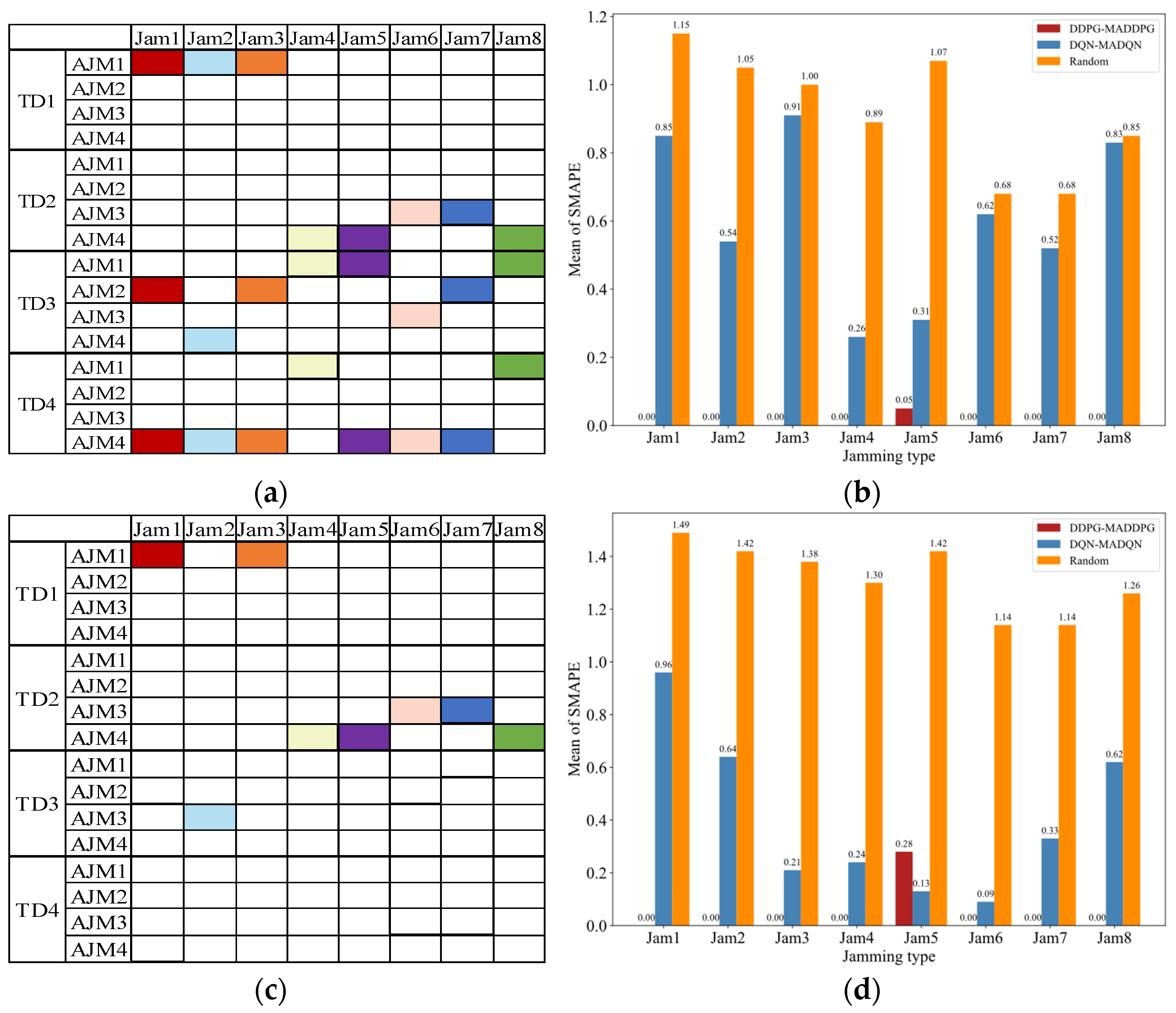
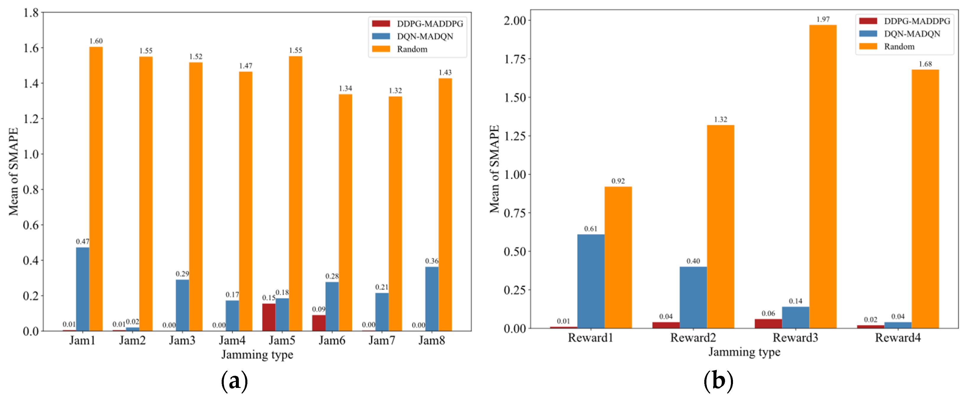
4.3. Decision Accuracy Performance Based on SMAPE

To verify the accuracy of the anti-jamming decision-making method, we calculated the decision-making error between the current anti-jamming policy $\pi \left(a_t\left|s_t\right.\right)$ and the optimal anti-jamming policy ${\pi }^{\ast }$. The symmetric mean absolute percentage error (SMAPE) was used as the criterion to characterize the decision-making error. It was defined as:

$$\mathrm{SMAPE}=\frac{100\%}{B}{\displaystyle \sum }_{b=1}^B\frac{\left|{\widehat{x}}_b-x_b\right|}{\left(\left|{\widehat{x}}_b\right|+\left|x_b\right|\right)/2}$$

(20)

where $b$ is the number of predicted data sets. $x_b$ is the true value of the $b\mathrm{th}$ sample, which is the optimal solution for the decision making. ${\widehat{x}}_b$ is the predicted value for the $b\mathrm{th}$ sample.

Figure 7 shows the anti-jamming strategy and the SMAPE value for decision-making objectives 1 and 2. For decision-making objective 1, the optimal decision-making result for each jamming is the cascade use of three ECCMs, as shown in Figure 7a. This is because decision-making objective 1 only considers the optimal anti-jamming effect and abandons the complexity brought by the increase in the number of ECCMs. The decision error in Figure 7b shows that the SMAPE of the DDPG-MADDPG algorithm suppressing jamming $Ja{m}_5$ is 0.05, and the other SMAPEs are all 0. However, the SMAPE of the DQN-MADQN algorithm is less than 0.5 when suppressing jamming $Ja{m}_4$ and $Ja{m}_5$, and the rest of the SMAPEs are greater than 0.5. The SMAPEs of the random decision making are all greater than 0.5. For decision-making objective 2, the optimal decision-making result for each jamming is the cascade use of three ECCMs, as shown in Figure 7c. For each jamming, the algorithm decides on one ECCM. This is because decision-making objective 2 only considers the average value of the anti-jamming effect. Compared with the strategy of cascading multiple ECCMs, the anti-jamming effect of one ECCM is smaller than the average value. The decision error in Figure 7d shows that the SMAPE of the DDPG-MADDPG algorithm suppressing jamming $Ja{m}_5$ is 0.28, and the other SMAPEs are all 0. However, the SMAPE of the DQN-MADQN algorithm is greater than 0.5 when jamming $Ja{m}_1$, $Ja{m}_2$ and $Ja{m}_8$ are suppressed, and the rest of the SMAPEs are less than 0.5. The SMAPEs of the random decision making are all greater than 0.5.

Figure 8 shows the anti-jamming strategy and SMAPE value for decision-making objectives 3 and 4. For decision-making objective 3, the optimal decision-making result is shown in Figure 8a. The optimal strategy to suppress jamming $Ja{m}_4$ is the ECCM $AJ{M}_4$ of transform sub-domain $T{D}_2$. The optimal strategy to suppress jamming $Ja{m}_1$, $Ja{m}_2$, $Ja{m}_3$, and $Ja{m}_5$ is the cascade use of two ECCMs. The optimal strategy to suppress jamming $Ja{m}_7$ and $Ja{m}_8$ is the cascade use of three ECCMs. This is because decision-making objective 3 not only considers the anti-jamming effect but also the complexity brought by the number of ECCMs. The decision error in Figure 8b shows that the SMAPE of the DDPG-MADDPG algorithm suppressing jamming is 0 for $Ja{m}_3$, $Ja{m}_4$, and $Ja{m}_8$. Although other SMAPEs are not 0, they are less than 0.25. However, the SMAPEs of the DQN-MADQN algorithm are 0 when $Ja{m}_1$, $Ja{m}_2$, $Ja{m}_6$, and $Ja{m}_7$ are suppressed, the SMAPEs are 0.67 when jamming $Ja{m}_8$ is suppressed, and the other SMAPEs are less than 0.25. The SMAPEs of the random algorithm are all greater than one. For decision-making objective 4, the optimal decision-making result is shown in Figure 8c. The optimal strategy for suppressing jamming $Ja{m}_1$ is the cascade use of two ECCMs. When suppressing the others, three ECCMs are chosen to be used in the cascade. Compared with decision-making objective 3, decision-making objective 4 focuses more on the importance of the anti-jamming effect. The decision error in Figure 8d shows that the SMAPEs of the DDPG-MADDPG algorithm suppress $Ja{m}_5$ and $Ja{m}_6$, which are less than 0.15. The SMAPEs when suppressing other jamming modes are 0. Although the SMAPEs when the DQN-MADQN algorithm suppresses $Ja{m}_7$ and $Ja{m}_8$ are 0, the SMAPEs when suppressing other jamming modes are greater than 0.1. The SMAPEs of the random algorithm are all greater than one.

For comparative analysis, we calculated the average SMAPEs, as shown in Figure 9. In Figure 9a, the average SMAPE of the DDPG-MADDPG algorithm is approximately 0, indicating that the decision-making results are approximately equal to the optimal anti-jamming strategy. The average SMAPE of the DQN-MADQN algorithm is greater than 0.1, indicating that it hardly found the optimal anti-jamming strategy. In Figure 9b, the average SMAPE of the DDPG-MADDPG algorithm is also approximately 0. When the decision-making objectives are 1, 2, and 3, the average SMAPE of the DQN-MADQN algorithm is greater than 0.1, indicating that it hardly found the optimal solution. Therefore, compared with DQN-MADQN, the decision error of DDPG-MADDPG is reduced by more than 85%.

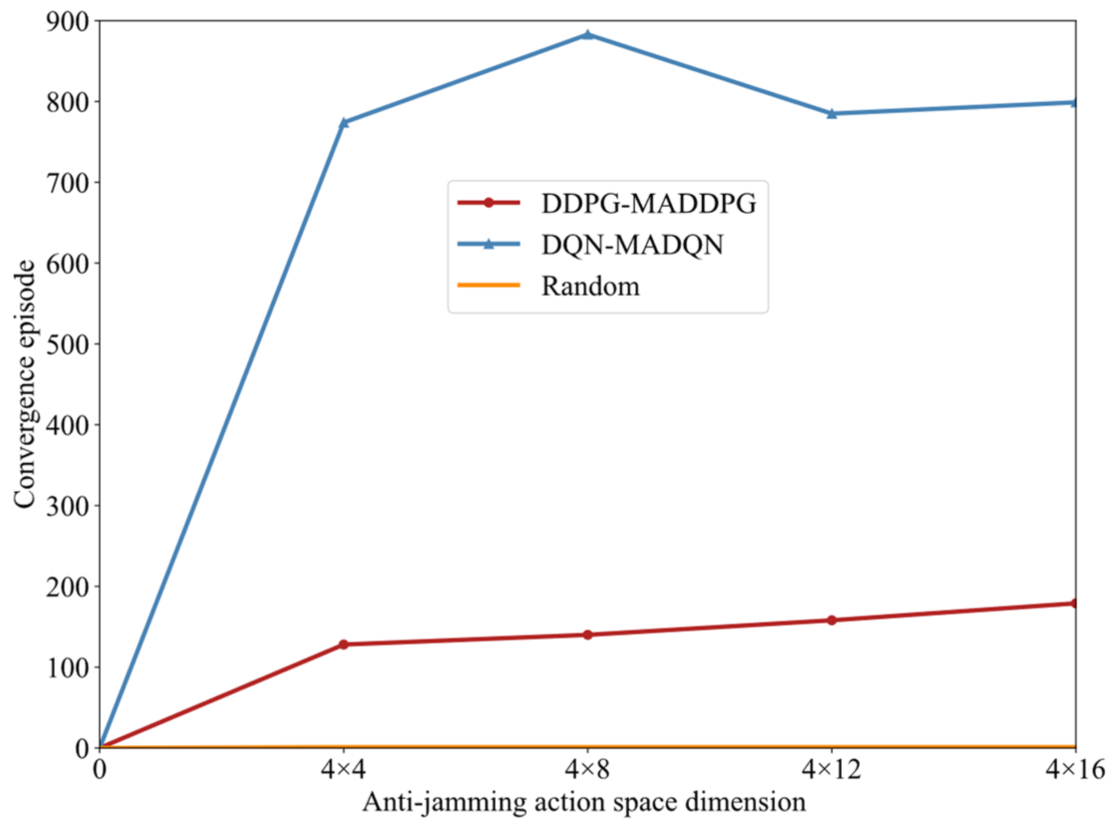
4.4. Generalization Performance Based on Large Action Space

To verify the generalization performance of the algorithm in large data dimensions, we expanded the action space of the algorithms based on decision-making objective 4. We set the anti-jamming action space to 4 × 4 (where $M=4,W=4$), 4 × 8 (where $M=4,W=8$), 4 × 12 (where $M=4,W=12$), and 4 × 16 (where $M=4,W=16$), respectively.

Under different anti-jamming action space dimensions, we observed the convergence episode of the reward function, as shown in Figure 10. The convergence episode of the DDPG-MADDPG algorithm was smaller than the convergence episode of the DQN-MADQN algorithm. As the dimension of the anti-jamming action space increased, the gap between the two became larger. The convergence episode of the DQN-MADQN was very unstable. When the action space dimension was 4 × 8, the convergence episode suddenly became larger and then became smaller, but the overall trend was upward. Because the random algorithm is a random decision method, there is no concept of convergence time. The decisions it makes are evenly distributed, so the curve is a straight line with one convergence episode. Therefore, the convergence time of the DDPG-MADDPG algorithm within 4×16 dimensions can be controlled within 200 convergence episodes. In conclusion, the DDPG-MADDPG algorithm has better scalability and stronger adaptability when dealing with the optimal selection problem of a high-dimensional knowledge base of ECCMs.

5. Conclusions

In this investigation, we proposed an intelligent radar anti-jamming decision-making method based on the DDPG-MADDPG algorithm. By establishing the working scenario of radar and jamming, we designed an intelligent radar anti-jamming decision-making model, and the decision-making process was formulated. Anti-jamming improvement factors play an important role in the problem of evaluating the performance of ECCMs, and the correlation matrix of jamming and anti-jamming is derived from it. With the correlation matrix of jamming and anti-jamming as prior knowledge, the DDPG-MADDPG algorithm was designed to generate an anti-jamming strategy. To verify the performance of the radar anti-jamming decision-making method based on the DDPG-MADDPG algorithm, it was compared with the anti-jamming decision-making method based on the DQN-MADQN algorithm and a random decision-making algorithm.

Four comparative experiments were performed: (1) We analyzed the loss function of the neural network to verify the robustness of the algorithms. The loss value of the DDPG-MADDPG model was restrained to 0 in the first 22 training times. However, the loss value of the DQN-MADQN model could hardly converge to 0. It was verified that the proposed method has superior robustness performance for different decision-making objectives. (2) The reward function was analyzed to verify the robust convergence performance of the algorithms. Among the four decision-making objectives, the reward values of the DDPG-MADDPG algorithm achieved convergence within 150 episodes. However, the DQN-MADQN algorithm needed to gradually converge after 800 episodes. This proves that the DDPG-MADDPG algorithm has a short convergence time, which can be improved by about 80%. (3) The anti-jamming decisions were performed for eight jamming modes, and the criterion based on SMAPE was used to evaluate the anti-jamming decision making accuracy. The average SMAPE of the DDPG-MADDPG algorithm was approximately 0, indicating that the decision-making results were approximately equal to the optimal anti-jamming strategy. Compared with the DQN-MADQN algorithm, the decision error of the DDPG-MADDPG algorithm was reduced by more than 85%. (4) We tested the convergence time of the algorithms at different action space dimensions. The convergence time of the DDPG-MADDPG algorithm within 4×16 dimensions can be controlled within 200 convergence episodes. However, the convergence time of the DQN-MADQN model reached 890 convergence episodes in the 4×8 dimensions. It can be seen that the DDPG-MADDPG algorithm still has excellent generalization performance at high dimensions.

In future research, we will design targeted intelligent radar anti-jamming decision-making methods based on the dynamic and varied scene of one jamming mode. The research results are and will be continuously put into the knowledge base. We will also obtain more data and expert knowledge through experiments to continuously enrich the database. In the end, we will study more generalized intelligent radar anti-jamming decision-making algorithms.

References

1. Geng, J.; Jiu, B.; Li, K.; Zhao, Y.; Liu, H.; Li, H. Radar and Jammer Intelligent Game under Jamming Power Dynamic Allocation. Remote Sens. 2023, 15, 581. [Google Scholar] [CrossRef]
2. Li, K.; Jiu, B.; Pu, W.; Liu, H.; Peng, X. Neural Fictitious Self-Play for Radar Antijamming Dynamic Game with Imperfect Information. IEEE Trans. Aerosp. Electron. Syst. 2022, 58, 5533–5547. [Google Scholar] [CrossRef]
3. Li, K.; Jiu, B.; Liu, H. Game Theoretic Strategies Design for Monostatic Radar and Jammer Based on Mutual Information. IEEE Access 2019, 7, 72257–72266. [Google Scholar] [CrossRef]
4. Feng, X.; Zhao, Z.; Li, F.; Cui, W.; Zhao, Y. Radar Phase-Coded Waveform Design with Local Low Range Sidelobes Based on Particle Swarm-Assisted Projection Optimization. Remote Sens. 2022, 14, 4186. [Google Scholar] [CrossRef]
5. Jin, M.H.; Yeo, S.-R.; Choi, H.H.; Park, C.; Lee, S.J. Jammer Identification Technique based on a Template Matching Method. J. Position. Navig. Timing 2014, 3, 45–51. [Google Scholar] [CrossRef]
6. Yu, W.; Sun, Y.; Wang, X.; Li, K.; Luo, J. Modeling and Analyzing of Fire-Control Radar Anti-Jamming Performance in the Complex Electromagnetic Circumstances. In Proceedings of the International Conference on Man-Machine-Environment System Engineering, Jinggangshan, China, 21–23 October 2017; Springer: Singapore, 2017. [Google Scholar] [CrossRef]
7. Guo, W.; Zhang, S.; Wang, Z. A method to evaluate radar effectiveness based on fuzzy analytic hierarchy process. In Proceedings of the 2008 Chinese Control and Decision Conference, Yantai, China, 2–4 July 2008. [Google Scholar] [CrossRef]
8. Xia, X.; Hao, D.; Wu, X. Optimal Waveform Design for Smart Noise Jamming. In Proceedings of the 7th International Conference on Education, Management, Information and Mechanical Engineering, Shenyang, China, 28–30 April 2017. [Google Scholar] [CrossRef]
9. Liu, Z.; Zhang, Q.; Li, K. A Smart Noise Jamming Suppression Method Based on Atomic Dictionary Parameter Optimization Decomposition. Remote Sens. 2022, 14, 1921. [Google Scholar] [CrossRef]
10. Liu, Y.-X.; Zhang, Q.; Xiong, S.-C.; Ni, J.-C.; Wang, D.; Wang, H.-B. An ISAR Shape Deception Jamming Method Based on Template Multiplication and Time Delay. Remote Sens. 2023, 15, 2762. [Google Scholar] [CrossRef]
11. Dai, H.; Zhao, Y.; Su, H.; Wang, Z.; Bao, Q.; Pan, J. Research on an Intra-Pulse Orthogonal Waveform and Methods Resisting Interrupted-Sampling Repeater Jamming within the Same Frequency Band. Remote Sens. 2023, 15, 3673. [Google Scholar] [CrossRef]
12. Zhan, H.; Wang, T.; Guo, T.; Su, X. An Anti-Intermittent Sampling Jamming Technique Utilizing the OTSU Algorithm of Random Orthogonal Sub-Pulses. Remote Sens. 2023, 15, 3080. [Google Scholar] [CrossRef]
13. Han, B.; Qu, X.; Yang, X.; Li, W.; Zhang, Z. DRFM-Based Repeater Jamming Reconstruction and Cancellation Method with Accurate Edge Detection. Remote Sens. 2023, 15, 1759. [Google Scholar] [CrossRef]
14. Kirk, B.H.; Narayanan, R.M.; Gallagher, K.A.; Martone, A.F.; Sherbondy, K.D. Avoidance of Time-Varying Radio Frequency Interference with Software-Defined Cognitive Radar. IEEE Trans. Aerosp. Electron. Syst. 2019, 55, 1090–1107. [Google Scholar] [CrossRef]
15. Wang, X.; Wang, S.; Liang, X.; Zhao, D.; Huang, J.; Xu, X.; Dai, B.; Miao, Q. Deep Reinforcement Learning: A Survey. IEEE Trans. Neural Networks Learn. Syst. 2022, 1–15. [Google Scholar] [CrossRef]
16. Feng, S.; Haykin, S. Cognitive Risk Control for Anti-Jamming V2V Communications in Autonomous Vehicle Networks. IEEE Trans. Veh. Technol. 2019, 68, 9920–9934. [Google Scholar] [CrossRef]
17. Lotfi, I.; Niyato, D.; Sun, S.; Dinh, H.T.; Li, Y.; Kim, D.I. Protecting Multi-Function Wireless Systems from Jammers with Backscatter Assistance: An Intelligent Strategy. IEEE Trans. Veh. Technol. 2021, 70, 11812–11826. [Google Scholar] [CrossRef]
18. Pourranjbar, A.; Kaddoum, G.; Ferdowsi, A.; Saad, W. Reinforcement Learning for Deceiving Reactive Jammers in Wireless Networks. IEEE Trans. Commun. 2021, 69, 3682–3697. [Google Scholar] [CrossRef]
19. Xiao, L.; Jiang, D.; Xu, D.; Zhu, H.; Zhang, Y.; Poor, H.V. Two-dimensional anti-jamming mobile communication based on reinforcement learning. IEEE Trans. Veh. Technol. 2018, 67, 9499–9512. [Google Scholar] [CrossRef]
20. Ailiya; Yi, W.; Varshney, P.K. Adaptation of Frequency Hopping Interval for Radar Anti-Jamming Based on Reinforcement Learning. IEEE Trans. Veh. Technol. 2022, 71, 12434–12449. [Google Scholar] [CrossRef]
21. Thornton, C.E.; Kozy, M.A.; Buehrer, R.M.; Martone, A.F.; Sherbondy, K.D. Deep Reinforcement Learning Control for Radar Detection and Tracking in Congested Spectral Environments. IEEE Trans. Cogn. Commun. Netw. 2020, 6, 1335–1349. [Google Scholar] [CrossRef]
22. Liu, P.; Liu, Y.; Huang, T.; Lu, Y.; Wang, X. Decentralized Automotive Radar Spectrum Allocation to Avoid Mutual Interference Using Reinforcement Learning. IEEE Trans. Aerosp. Electron. Syst. 2020, 57, 190–205. [Google Scholar] [CrossRef]
23. Selvi, E.; Buehrer, R.M.; Martone, A.; Sherbondy, K. Reinforcement Learning for Adaptable Bandwidth Tracking Radars. IEEE Trans. Aerosp. Electron. Syst. 2020, 56, 3904–3921. [Google Scholar] [CrossRef]
24. Feng, C.; Fu, X.; Wang, Z.; Dong, J.; Zhao, Z.; Pan, T. An Optimization Method for Collaborative Radar Antijamming Based on Multi-Agent Reinforcement Learning. Remote Sens. 2023, 15, 2893. [Google Scholar] [CrossRef]
25. Li, K.; Jiu, B.; Liu, H.; Liang, S. Reinforcement learning based anti-jamming frequency hopping strategies design for cognitive radar. In Proceedings of the 2018 IEEE International Conference on Signal Processing, Communications and Computing (ICSPCC), Qingdao, China, 14–16 September 2018; pp. 1–5. [Google Scholar]
26. Li, K.; Jiu, B.; Liu, H. Deep Q-Network based anti-Jamming strategy design for frequency agile radar. In Proceedings of the International Radar Conference (RADAR), Toulon, France, 23–27 September 2019. [Google Scholar] [CrossRef]
27. Ak, S.; Brüggenwirth, S. Avoiding Jammers: A Reinforcement Learning Approach. In Proceedings of the 2020 IEEE International Radar Conference (RADAR), Washington, DC, USA, 28–30 April 2020; pp. 321–326. [Google Scholar]
28. Li, K.; Jiu, B.; Wang, P.; Liu, H.; Shi, Y. Radar active antagonism through deep reinforcement learning: A Way to address the challenge of mainlobe jamming. Signal Process. 2021, 186, 108130. [Google Scholar] [CrossRef]
29. Li, K.; Jiu, B.; Liu, H.; Pu, W. Robust Antijamming Strategy Design for Frequency-Agile Radar against Main Lobe Jamming. Remote Sens. 2021, 13, 3043. [Google Scholar] [CrossRef]
30. Geng, J.; Jiu, B.; Li, K.; Zhao, Y.; Liu, H. Reinforcement Learning Based Radar Anti-Jamming Strategy Design against a Non-Stationary Jammer. In Proceedings of the 2022 IEEE International Conference on Signal Processing, Communications and Computing (ICSPCC), Xi’an, China, 25–27 October 2022. [Google Scholar] [CrossRef]
31. He, X.; Liao, K.; Peng, S.; Tian, Z.; Huang, J. Interrupted-Sampling Repeater Jamming-Suppression Method Based on a Multi-Stages Multi-Domains Joint Anti-Jamming Depth Network. Remote Sens. 2022, 14, 3445. [Google Scholar] [CrossRef]
32. Sharma, H.; Kumar, N.; Tekchandani, R. Mitigating Jamming Attack in 5G Heterogeneous Networks: A Federated Deep Reinforcement Learning Approach. IEEE Trans. Veh. Technol. 2023, 72, 2439–2452. [Google Scholar] [CrossRef]
33. Du, Y.; Zandi, H.; Kotevska, O.; Kurte, K.; Munk, J.; Amasyali, K.; Mckee, E.; Li, F. Intelligent multi-zone residential HVAC control strategy based on deep reinforcement learning. Appl. Energy 2021, 281, 116117. [Google Scholar] [CrossRef]
34. Zehni, M.; Zhao, Z. An Adversarial Learning Based Approach for 2D Unknown View Tomography. IEEE Trans. Comput. Imaging 2022, 8, 705–720. [Google Scholar] [CrossRef]
35. Peng, H.; Shen, X. Multi-Agent Reinforcement Learning Based Resource Management in MEC- and UAV-Assisted Vehicular Networks. IEEE J. Sel. Areas Commun. 2021, 39, 131–141. [Google Scholar] [CrossRef]
36. Johnston, S.L. The ECCM improvement factor (EIF)–Illustrative examples, applications, and considerations in its utilization in radar ECCM performance assessment. In Proceedings of the International Conference on Radar, Nanjing, China, 4–7 November 1986. [Google Scholar]
37. Liu, X.; Yang, J.; Hou, B.; Lu, J.; Yao, Z. Radar seeker performance evaluation based on information fusion method. SN Appl. Sci. 2020, 2, 674. [Google Scholar] [CrossRef]
38. Wang, X.; Zhang, S.; Zhu, L.; Chen, S.; Zhao, H. Research on anti-Narrowband AM jamming of Ultra-wideband impulse radio detection radar based on improved singular spectrum analysis. Measurement 2022, 188, 110386. [Google Scholar] [CrossRef]
39. Li, T.; Wang, Z.; Liu, J. Evaluating Effect of Blanket Jamming on Radar Via Robust Time-Frequency Analysis and Peak to Average Power Ratio. IEEE Access 2020, 8, 214504–214519. [Google Scholar] [CrossRef]
40. Xing, H.; Xing, Q.; Wang, K. Radar Anti-Jamming Countermeasures Intelligent Decision-Making: A Partially Observable Markov Decision Process Approach. Aerospace 2023, 10, 236. [Google Scholar] [CrossRef]
41. Wang, F.; Liu, D.; Liu, P.; Li, B. A Research on the Radar Anti-jamming Evaluation Index System. In Proceedings of the 2015 International Conference on Applied Science and Engineering Innovation, Jinan, China, 30–31 August 2015. [Google Scholar]
42. Lillicrap, T.; Hunt, J.; Pritzel, A. Continuous control with deep reinforcement learning. arXiv 2015, arXiv:1509.02971. [Google Scholar]
43. Watkins, C.J.C.H.; Dayan, P. Q-learning. Mach. Learn. 1992, 8, 279–292. [Google Scholar]
44. Mnih, V.; Kavukcuoglu, K.; Silver, D.; Rusu, A.A.; Veness, J.; Bellemare, M.G.; Graves, A.; Riedmiller, M.; Fidjeland, A.K.; Ostrovski, G.; et al. Human-level control through deep reinforcement learning. Nature 2015, 518, 529–533. [Google Scholar] [CrossRef] [PubMed]
45. Lowe, R.; Wu, Y.; Tamar, A.; Harb, J.; Abbeel, P.; Mordatch, I. Multi-agent actor-critic for mixed cooperative-competitive environments. In Proceedings of the 31st International Conference on Neural Information Processing Systems, Long Beach, CA, USA, 4–9 December 2017. [Google Scholar]
46. Jang, E.; Gu, S.; Poole, B. Categorical reparameterization with gumbel-softmax. arXiv 2016, arXiv:1611.01144. [Google Scholar]
47. Rasheed, F.; Yau, K.-L.A.; Low, Y.-C. Deep reinforcement learning for traffic signal control under disturbances: A case study on Sunway city, Malaysia. Futur. Gener. Comput. Syst. 2020, 109, 431–445. [Google Scholar] [CrossRef]
Figure 1. The working scenario of radar and jamming.
Remotesensing 15 04046 g001
Figure 2. Intelligent radar anti-jamming decision-making model.
Remotesensing 15 04046 g002
Figure 3. The dual RL model of DDPG-MADDPG.
Remotesensing 15 04046 g003
Figure 4. The curve of loss changing with training times. (a), (b), (c) and (d) are the training results when the decision-making objectives are 1, 2, 3, and 4, respectively. DDPG-MADDPG consists of four networks: the actor network of the outer DDPG, the critic network of the outer DDPG, the actor network of the inner MADDPG, and the critic network of the inner MADDPG. DQN-MADQN consists of two networks: the outer DQN network and the inner MADQN network.
Remotesensing 15 04046 g004
Figure 5. The curve of loss changing with 1–30 training times. (a), (b), (c) and (d) are the training results with 1–30 training times when the decision-making objectives are 1, 2, 3, and 4, respectively. DDPG-MADDPG consists of four networks: the actor network of the outer DDPG, the critic network of the outer DDPG, the actor network of the inner MADDPG, and the critic network of the inner MADDPG. DQN-MADQN consists of two networks: the outer DQN network and the inner MADQN network.
Remotesensing 15 04046 g005
Figure 6. The curve of reward changing with episodes. (a), (b), (c) and (d) are the training results when the decision-making objectives are 1, 2, 3, and 4, respectively.
Remotesensing 15 04046 g006
Figure 7. The optimal anti-jamming strategy and decision-making errors based on SMAPE. (a,c) show the optimal anti-jamming strategy determined by the DDPG-MADDPG algorithm for decision-making objectives 1 and 2. We mark the ECCMs selected by the algorithm in color. (b,d) show the decision-making errors based on SMAPE for decision-making objectives 1 and 2.
Remotesensing 15 04046 g007
Figure 8. The optimal anti-jamming strategy and decision-making errors based on SMAPE. (a,c) show the optimal anti-jamming strategy determined by the DDPG-MADDPG algorithm for decision-making objectives 3 and 4. We mark the ECCMs selected by the algorithm in color. (b,d) show the decision-making errors based on SMAPE for decision-making objectives 3 and 4.
Remotesensing 15 04046 g008
Figure 9. The average SMAPEs. (a) is the mean of the SMAPE obtained under the four decision-making objectives according to different jamming modes. (b) is the mean of the SMAPE obtained under the eight jamming modes according to different decision-making objectives.
Remotesensing 15 04046 g009
Figure 10. The convergence episode of different action space dimensions.
Remotesensing 15 04046 g010