
Dimensionality Reduction and Anomaly Detection Based on Kittler’s Taxonomy: Analyzing Water Bodies in Two Dimensional Spaces

 , , , ,
  and
and
Abstract
:1. Introduction
2. Materials and Methods
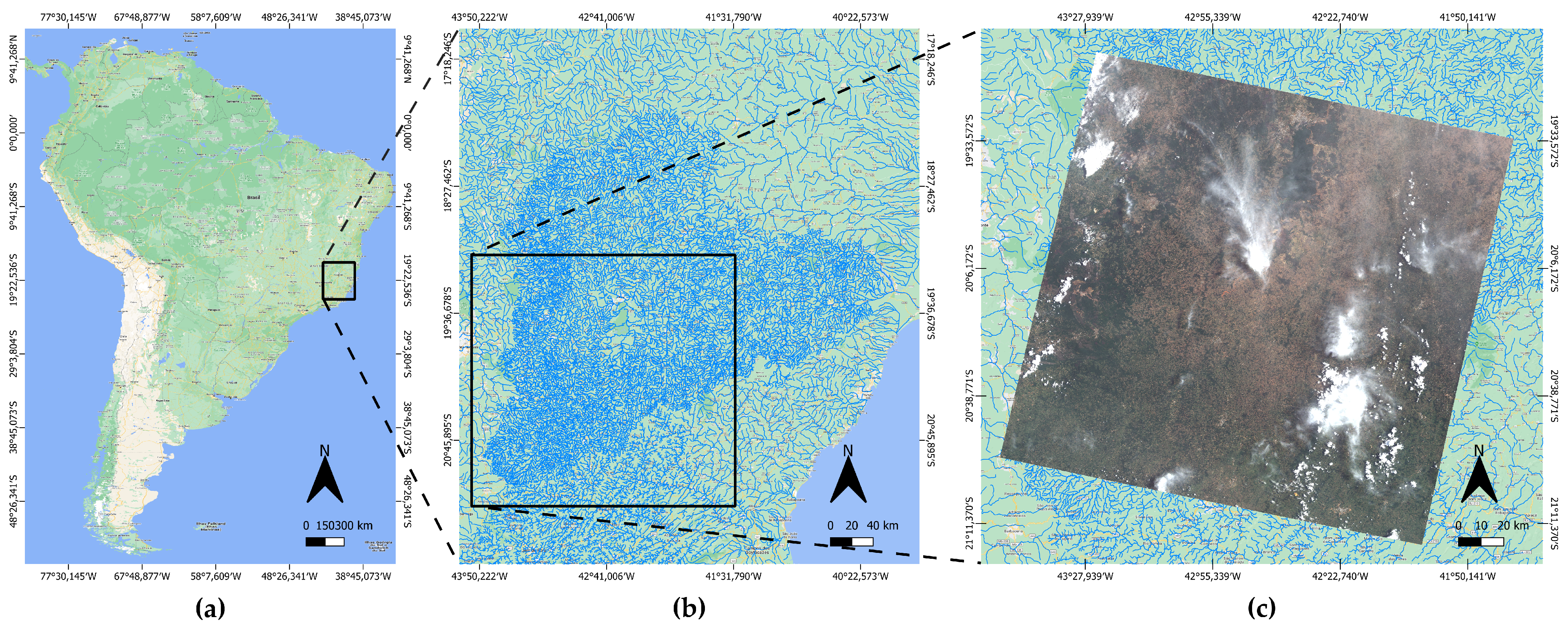
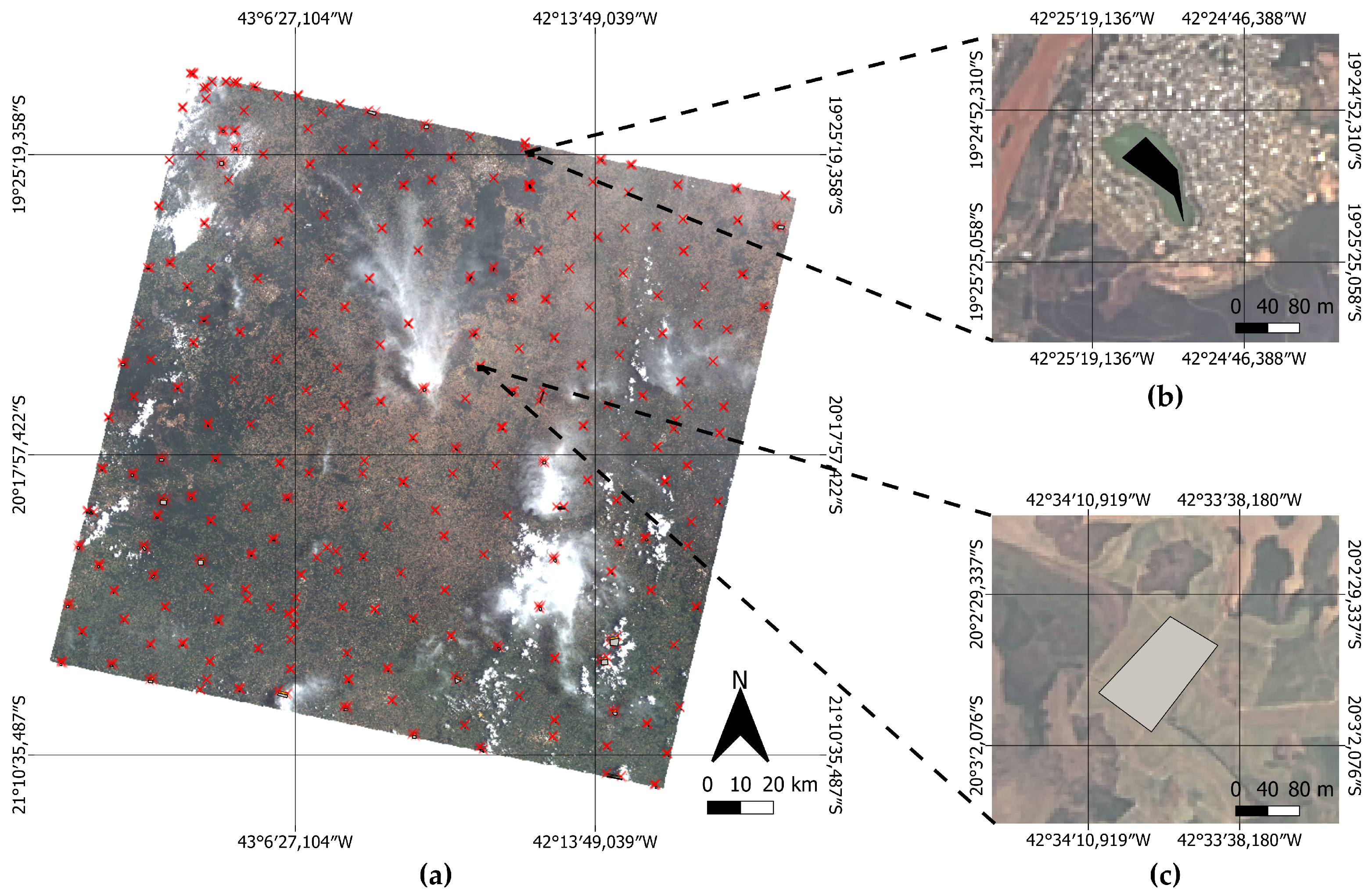
2.1. Study Area
2.2. Materials
2.3. Conceptualization
2.3.1. Dimensionality Reduction
2.3.2. Principal Component Analysis (PCA)
2.3.3. Multi- and Hyperspectral Images
2.3.4. Classification
2.3.5. Kittler’s Taxonomy
- Unexpected structure and structural components: this category of anomaly is related to a complete or partial change of the study area, i.e., of the domain. In this case, the observation differs considerably from the reference models of the classifiers in terms of its structure (which defines its shape) and components (which together make up the structure). Let us consider a model created to classify pixels in an image into “water” and “non-water” classes. During the classification, when analyzing a river that belongs to the image, if this river has undergone a change of domain, for example, it received a considerable amount of ore tailings, the classifier that was able to identify the river as water may fail, since the structure and components of this river are unexpected (water was expected and now it has turned to mud). This example was studied and published in [17]. Both the referred study [17] and any other study that applies anomaly detection based on Kittler’s Taxonomy to the analysis of water bodies (including this study) are very important to help preserve water resources. Clean water and sanitation correspond to the 6th goal of the UN Sustainable Development Goals [30]. This goal has received considerable critical attention from the scientific community to investigate and publish studies in order to help ensure the availability and the sustainable management of water resources and sanitation for the world [31,32,33,34,35].
- Unexpected structural component: this other category of anomaly is related to the lack of attributes in the model characteristics (only a subset of object models is used), i.e., the lack of relevant information leads to the occurrence of this type of anomaly. For example, the application of any filter may be responsible for eliminating features relevant to the model to classify an object as belonging to a certain type of anomaly, since the entire universe of features was not contemplated.
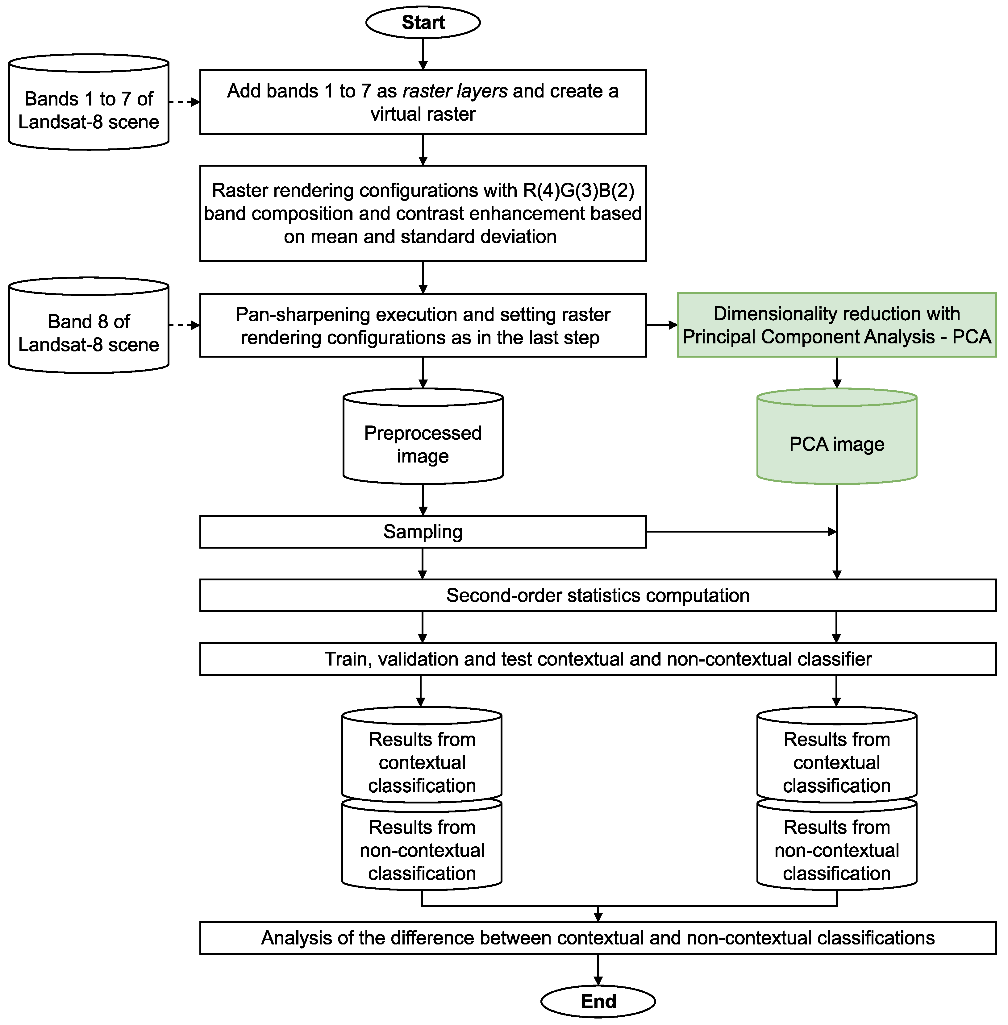
2.4. Methodology
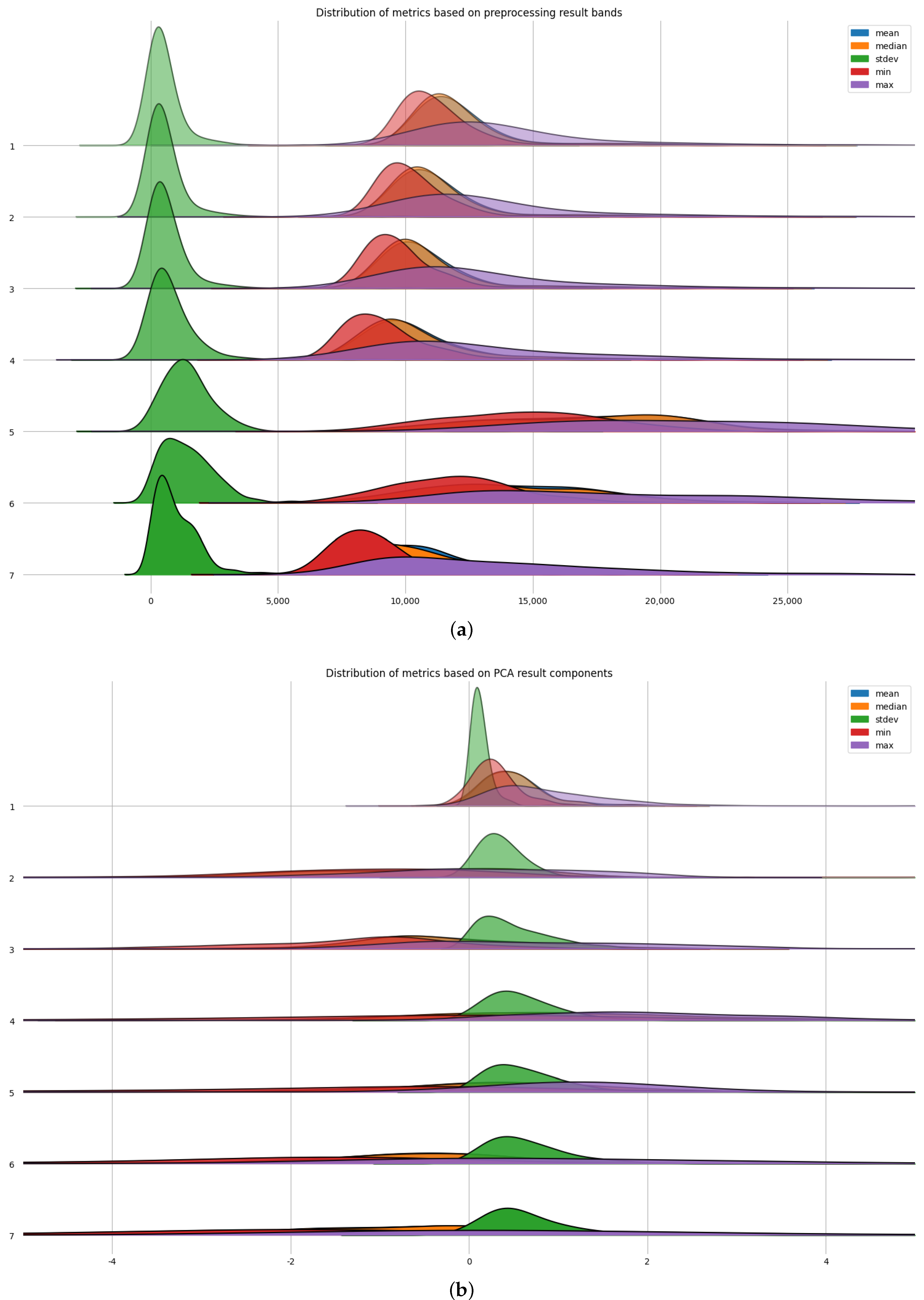
3. Results
4. Discussion
5. Conclusions
Author Contributions
Funding
Data Availability Statement
Acknowledgments
Conflicts of Interest
Appendix A. Processing Parameters
Appendix A.1. Pre-Processing
Appendix A.2. Dimensionality Reduction
- Rescale Output: no;
- Algorithm: pca;
- Option Perform pca whitening: checked (True);
- Number of Components: 0, indicating that all components will be kept;
- Option Center and reduce data: unchecked (False).
Appendix A.3. Classification
- Maximum training sample size per class: 1000;
- Maximum validation sample size per class: 1000;
- Bound sample number by minimum: 1;
- Training and validation sample ratio: ;
- Name of the discrimination field (the name of the field containing the classes in the collected samples file, a shapefile): Class;
- Default elevation: 0;
- Random seed: 0.
- Boost type: real;
- Weak count: 100;
- Weight Trim Rate: ;
- Maximum depth of the tree: 1.
- Maximum depth of the tree: 65,535;
- Minimum number of samples in each node: 10;
- Termination criteria for regression tree: ;
- Cluster possible values of a categorical variable into K <= cat clusters to find a suboptimal split: 10;
- Option Set Use1seRule flag to false: checked (True);
- Option Set TruncatePrunedTree flag to false: checked (True).
Appendix A.4. Feature Extraction
References
- Tiouiouine, A.; Yameogo, S.; Valles, V.; Barbiero, L.; Dassonville, F.; Moulin, M.; Bouramtane, T.; Bahaj, T.; Morarech, M.; Kacimi, I. Dimension Reduction and Analysis of a 10-Year Physicochemical and Biological Water Database Applied to Water Resources Intended for Human Consumption in the Provence-Alpes-Côte d’Azur Region, France. Water 2020, 12, 525. [Google Scholar] [CrossRef]
- Wang, G.; Lauri, F.; Hajjam El Hassani, A. A Study of Dimensionality Reduction’s Influence on Heart Disease Prediction. In Proceedings of the 2021 12th International Conference on Information, Intelligence, Systems & Applications (IISA), Chania Crete, Greece, 12–14 July 2021; pp. 1–6. [Google Scholar] [CrossRef]
- Sameer, Y.M.; Abed, A.N.; Sayl, K.N. Geomatics-based approach for highway route selection. Appl. Geomat. 2023, 15, 161–176. [Google Scholar] [CrossRef]
- Fowler, J.E.; Du, Q.; Zhu, W.; Younan, N.H. Classification performance of random-projection-based dimensionality reduction of hyperspectral imagery. In Proceedings of the 2009 IEEE International Geoscience and Remote Sensing Symposium, Cape Town, South Africa, 12–17 July 2009; Volume 5, pp. V-76–V-79. [Google Scholar] [CrossRef]
- Ghosh, S.; Pramanik, P. A Combined Framework for Dimensionality Reduction of Hyperspectral Images using Feature Selection and Feature Extraction. In Proceedings of the 2019 IEEE Recent Advances in Geoscience and Remote Sensing: Technologies, Standards and Applications (TENGARSS), Kochi, India, 17–20 October 2019; pp. 39–44. [Google Scholar] [CrossRef]
- Bilius, L.B.; Pentiuc, S.G. Tensor-Based and Projection-Based Methods for Dimensionality Reduction of Hyperspectral Images. In Proceedings of the 2022 International Conference on Development and Application Systems (DAS), Suceava, Romania, 26–28 May 2022; pp. 167–170. [Google Scholar] [CrossRef]
- Sellami, A.; Farah, M. Comparative study of dimensionality reduction methods for remote sensing images interpretation. In Proceedings of the 2018 4th International Conference on Advanced Technologies for Signal and Image Processing (ATSIP), Sousse, Tunisia, 21–24 March 2018; pp. 1–6. [Google Scholar] [CrossRef]
- Avramovic, A.; Risojevic, V. Descriptor dimensionality reduction for aerial image classification. In Proceedings of the 2011 18th International Conference on Systems, Signals and Image Processing, Sarajevo, Bosnia, 16–18 June 2011; pp. 1–4. [Google Scholar]
- Journaux, L.; Tizon, X.; Foucherot, I.; Gouton, P. Dimensionality Reduction Techniques: An Operational Comparison On Multispectral Satellite Images Using Unsupervised Clustering. In Proceedings of the Proceedings of the 7th Nordic Signal Processing Symposium—NORSIG 2006, Reykjavik, Iceland, 7–9 June 2006; pp. 242–245. [Google Scholar] [CrossRef]
- Grobler, T.; Kleynhans, W.; Salmon, B. Empirically Comparing Two Dimensionality Reduction Techniques – PCA and FFT: A Settlement Detection Case Study in the Gauteng Province of South Africa. In Proceedings of the IGARSS 2019—2019 IEEE International Geoscience and Remote Sensing Symposium, Yokohama, Japan, 28 July–2 August 2019; pp. 3329–3332. [Google Scholar] [CrossRef]
- Navin, M.S.; Agilandeeswari, L.; Anjaneyulu, G. Dimensionality Reduction and Vegetation Monitoring On LISS III Satellite Image Using Principal Component Analysis and Normalized Difference Vegetation Index. In Proceedings of the 2020 International Conference on Emerging Trends in Information Technology and Engineering (ic-ETITE), Vellore, India, 24–25 February 2020; pp. 1–5. [Google Scholar] [CrossRef]
- Yang, X.; Xu, W.d.; Liu, H.; Zhu, L.y. Research on Dimensionality Reduction of Hyperspectral Image under Close Range. In Proceedings of the 2019 International Conference on Communications, Information System and Computer Engineering (CISCE), Haikou, China, 5–7 July 2019; pp. 171–174. [Google Scholar] [CrossRef]
- Zhang, X.; Huyan, N.; Zhou, N.; An, J. Semi-supervised sparse dimensionality reduction for hyperspectral image classification. In Proceedings of the 2016 IEEE Region 10 Conference (TENCON), Singapore, 22–25 November 2016; pp. 2830–2833. [Google Scholar] [CrossRef]
- Gu, Y.; Wang, Q. Discriminative graph-based dimensionality reduction for hyperspectral image classification. In Proceedings of the 2016 8th Workshop on Hyperspectral Image and Signal Processing: Evolution in Remote Sensing (WHISPERS), Los Angeles, CA, USA, 21–24 August 2016; pp. 1–5. [Google Scholar] [CrossRef]
- Liang, L.; Xia, Y.; Xun, L.; Yan, Q.; Zhang, D. Class-Probability Based Semi-Supervised Dimensionality Reduction for Hyperspectral Images. In Proceedings of the 2018 IEEE 9th International Conference on Software Engineering and Service Science (ICSESS), Beijing, China, 23–25 November 2018; pp. 460–463. [Google Scholar] [CrossRef]
- Kittler, J.; Christmas, W.; de Campos, T.; Windridge, D.; Yan, F.; Illingworth, J.; Osman, M. Domain Anomaly Detection in Machine Perception: A System Architecture and Taxonomy. IEEE Trans. Pattern Anal. Mach. Intell. 2014, 36, 845–859. [Google Scholar] [CrossRef] [PubMed]
- Dias, M.A.; Silva, E.A.d.; Azevedo, S.C.d.; Casaca, W.; Statella, T.; Negri, R.G. An Incongruence-Based Anomaly Detection Strategy for Analyzing Water Pollution in Images from Remote Sensing. Remote Sens. 2020, 12, 43. [Google Scholar] [CrossRef]
- Dias, M.A.; Marinho, G.C.; Negri, R.G.; Casaca, W.; Muñoz, I.B.; Eler, D.M. A Machine Learning Strategy Based on Kittler’s Taxonomy to Detect Anomalies and Recognize Contexts Applied to Monitor Water Bodies in Environments. Remote Sens. 2022, 14, 2222. [Google Scholar] [CrossRef]
- USGS—The United States Geological Survey, “Earth Explorer”. Available online: https://earthexplorer.usgs.gov/ (accessed on 5 August 2023).
- Marcílio-Jr, W.E.; Eler, D.M. Explaining dimensionality reduction results using Shapley values. Expert Syst. Appl. 2021, 178, 115020. [Google Scholar] [CrossRef]
- Crosta, A. Processamento Digital de Imagens de Sensoriamento Remoto; UNICAMP/Instituto de Geociências: Campinas, Brazilian, 1999. [Google Scholar]
- Bishop, C.M. Pattern Recognition and Machine Learning (Information Science and Statistics); Springer: Berlin/Heidelberg, Germany, 2006. [Google Scholar]
- Richards, J.; Jia, X. Remote Sensing Digital Image Analysis; Springer: Berlin/Heidelberg, Germany, 1999. [Google Scholar] [CrossRef]
- Boosting—OpenCV Documentation. Available online: https://docs.opencv.org/2.4/modules/ml/doc/boosting.html (accessed on 11 March 2023).
- Decision Trees—OpenCV Documentation. Available online: https://docs.opencv.org/2.4/modules/ml/doc/decision_trees.html (accessed on 11 March 2023).
- Weinshall, D.; Zweig, A.; Hermansky, H.; Kombrink, S.; Ohl, F.W.; Anemüller, J.; Bach, J.H.; Van Gool, L.; Nater, F.; Pajdla, T.; et al. Beyond Novelty Detection: Incongruent Events, When General and Specific Classifiers Disagree. IEEE Trans. Pattern Anal. Mach. Intell. 2012, 34, 1886–1901. [Google Scholar] [CrossRef] [PubMed]
- Kittler, J.; Zor, C. A measure of surprise for incongruence detection. In Proceedings of the 2nd IET International Conference on Intelligent Signal Processing 2015 (ISP), London, UK, 1–2 December 2015; pp. 1–6. [Google Scholar] [CrossRef]
- Ponti, M.; Kittler, J.; Riva, M.; de Campos, T.; Zor, C. A decision cognizant Kullback–Leibler divergence. Pattern Recognit. 2017, 61, 470–478. [Google Scholar] [CrossRef]
- Kittler, J.; Zor, C. Delta Divergence: A Novel Decision Cognizant Measure of Classifier Incongruence. IEEE Trans. Cybern. 2019, 49, 2331–2343. [Google Scholar] [CrossRef] [PubMed]
- United Nations Department of Economic and Social Affairs (UN DESA). The Sustainable Development Goals Report 2022–July 2022; United Nations Publications: New York, NY, USA, 2022. [Google Scholar]
- Assaf, A.T.; Sayl, K.N.; Adham, A. Surface Water Detection Method for Water Resources Management. J. Phys. Conf. Ser. 2021, 1973, 012149. [Google Scholar] [CrossRef]
- Adham, A.; Sayl, K.N.; Abed, R.; Abdeladhim, M.A.; Wesseling, J.G.; Riksen, M.; Fleskens, L.; Karim, U.; Ritsema, C.J. A GIS-based approach for identifying potential sites for harvesting rainwater in the Western Desert of Iraq. Int. Soil Water Conserv. Res. 2018, 6, 297–304. [Google Scholar] [CrossRef]
- Shen, J.; Li, J.; Zhang, Y.; Song, J. Farmers’ Water Poverty Measurement and Analysis of Endogenous Drivers. Water Resour. Manag. 2023, 1–18. [Google Scholar] [CrossRef]
- Sulaiman, S.O.; Kamel, A.H.; Sayl, K.N.; Alfadhel, M.Y. Water resources management and sustainability over the Western desert of Iraq. Environ. Earth Sci. 2019, 78, 495. [Google Scholar] [CrossRef]
- Sayl, K.N.; Muhammad, N.S.; Yaseen, Z.M.; El-shafie, A. Estimation the Physical Variables of Rainwater Harvesting System Using Integrated GIS-Based Remote Sensing Approach. Water Resour. Manag. 2016, 30, 3299–3313. [Google Scholar] [CrossRef]
- Gonzales, R.C.; Wintz, P. Digital Image Processing, 2nd ed.; Addison-Wesley Longman Publishing Co., Inc.: St, Boston, MA, USA, 1987. [Google Scholar]
- Documentation for QGIS 2.18. Available online: https://docs.qgis.org/2.18/en/docs/ (accessed on 11 March 2023).
- Vivone, G.; Alparone, L.; Chanussot, J.; Dalla Mura, M.; Garzelli, A.; Licciardi, G.A.; Restaino, R.; Wald, L. A Critical Comparison Among Pansharpening Algorithms. IEEE Trans. Geosci. Remote Sens. 2015, 53, 2565–2586. [Google Scholar] [CrossRef]
- Mhangara, P.; Mapurisa, W.; Mudau, N. Comparison of Image Fusion Techniques Using Satellite Pour l’Observation de la Terre (SPOT) 6 Satellite Imagery. Appl. Sci. 2020, 10, 1881. [Google Scholar] [CrossRef]
- Xu, Q.; Li, B.; Zhang, Y.; Ding, L. High-Fidelity Component Substitution Pansharpening by the Fitting of Substitution Data. IEEE Trans. Geosci. Remote Sens. 2014, 52, 7380–7392. [Google Scholar] [CrossRef]
- Documentation for Orfeo ToolBox 6.4. Available online: https://www.orfeo-toolbox.org/CookBook-6.4/ (accessed on 11 March 2023).
- Shen, L.; Li, C. Water body extraction from Landsat ETM+ imagery using adaboost algorithm. In Proceedings of the 2010 18th International Conference on Geoinformatics, Beijing, China, 18–20 June 2010; pp. 1–4. [Google Scholar] [CrossRef]
- Yi-bin, L.; Ying-ying, W.; Xue-wen, R. Improvement of ID3 algorithm based on simplified information entropy and coordination degree. In Proceedings of the 2017 Chinese Automation Congress (CAC), Jinan, China, 20–22 October 2017; pp. 1526–1530. [Google Scholar] [CrossRef]
- Swain, P.H.; Hauska, H. The decision tree classifier: Design and potential. IEEE Trans. Geosci. Electron. 1977, 15, 142–147. [Google Scholar] [CrossRef]
- Documentation for QGIS 3.22. Available online: https://docs.qgis.org/3.22/en/docs/ (accessed on 11 March 2023).
- Documentation for Orfeo ToolBox 7.4. Available online: https://www.orfeo-toolbox.org/CookBook-7.4/ (accessed on 11 March 2023).

| Produced Labels | |||||
|---|---|---|---|---|---|
| 0 (No-Water) | 1 (Water) | ||||
| Pre-processing | DT | Reference labels | 0 (no-water) | 6190 | 129 |
| 1 (water) | 107 | 6212 | |||
| Boost | Reference labels | 0 (no-water) | 6245 | 74 | |
| 1 (water) | 130 | 6189 | |||
| PCA | DT | Reference labels | 0 (no-water) | 6224 | 95 |
| 1 (water) | 62 | 6257 | |||
| Boost | Reference labels | 0 (no-water) | 6195 | 124 | |
| 1 (water) | 94 | 6225 | |||
Disclaimer/Publisher’s Note: The statements, opinions and data contained in all publications are solely those of the individual author(s) and contributor(s) and not of MDPI and/or the editor(s). MDPI and/or the editor(s) disclaim responsibility for any injury to people or property resulting from any ideas, methods, instructions or products referred to in the content. |
© 2023 by the authors. Licensee MDPI, Basel, Switzerland. This article is an open access article distributed under the terms and conditions of the Creative Commons Attribution (CC BY) license (https://creativecommons.org/licenses/by/4.0/).
Share and Cite
Marinho, G.C.; Júnior, W.E.M.; Dias, M.A.; Eler, D.M.; Negri, R.G.; Casaca, W. Dimensionality Reduction and Anomaly Detection Based on Kittler’s Taxonomy: Analyzing Water Bodies in Two Dimensional Spaces. Remote Sens. 2023, 15, 4085. https://doi.org/10.3390/rs15164085
Marinho GC, Júnior WEM, Dias MA, Eler DM, Negri RG, Casaca W. Dimensionality Reduction and Anomaly Detection Based on Kittler’s Taxonomy: Analyzing Water Bodies in Two Dimensional Spaces. Remote Sensing. 2023; 15(16):4085. https://doi.org/10.3390/rs15164085
Chicago/Turabian StyleMarinho, Giovanna Carreira, Wilson Estécio Marcílio Júnior, Mauricio Araujo Dias, Danilo Medeiros Eler, Rogério Galante Negri, and Wallace Casaca. 2023. "Dimensionality Reduction and Anomaly Detection Based on Kittler’s Taxonomy: Analyzing Water Bodies in Two Dimensional Spaces" Remote Sensing 15, no. 16: 4085. https://doi.org/10.3390/rs15164085
APA StyleMarinho, G. C., Júnior, W. E. M., Dias, M. A., Eler, D. M., Negri, R. G., & Casaca, W. (2023). Dimensionality Reduction and Anomaly Detection Based on Kittler’s Taxonomy: Analyzing Water Bodies in Two Dimensional Spaces. Remote Sensing, 15(16), 4085. https://doi.org/10.3390/rs15164085