Rapid Detection of Iron Ore and Mining Areas Based on MSSA-BNVTELM, Visible—Infrared Spectroscopy, and Remote Sensing

Abstract

The accuracy and rapidity of total iron content (TFE) analysis can accelerate iron ore production. Although the conventional TFE detection methods are accurate, its detection speed presents difficulties in meeting production requirements. Therefore, this paper proposes a method of TFE detection based on reflectance spectroscopy (wavelength range: 340–2500 nm) and remote sensing. Firstly, spectral experiments were conducted on iron ore using the HR SVC-1024 spectrometer to obtain spectral data for each sample. Then, the spectra were smoothed and dimensionally reduced by using wavelet transform and principal component analysis. To improve the detection accuracy of TFE, a two hidden layer extreme learning machine with variable neuron nodes based on an improved sparrow search algorithm and batch normalization optimization (MSSA-BNVTELM) is proposed. According to the experimental results, MSSA-BNVTELM exhibited superior detection accuracy in comparison to other algorithms. In addition, this research established a remote sensing detection model using Sentinel-2 data and MSSA-BNVTEM to detect the distribution of TFE in the mining area. The distribution of TFE in the mine area was plotted based on the detection results. The results show that the remote sensing of the mine area can be useful for detection of the TFE distribution, providing assistance for the mining plan.

1. Introduction

In the mining process, iron ore needs to be matched and blended in a specific proportion to meet the quality requirements of the ore product. Iron ores with different total iron content (TFE) are blended to increase the output of qualified ore, improve the economic efficiency of the enterprise, and maximize the utilization of iron ore [1,2]. Therefore, it is crucial to detect the TFE of iron ore during the ore preparation process. Although the chemical spot-drop method can accurately determine the TFE of iron ore, its low detection efficiency and high cost make it impractical for large-scale implementation in mining [3,4].

Spectroscopy detection enables fast and non-destructive detection, making it widely used in ore detection [5]. Compared with chemical spotting and flame atomic absorption [6], spectroscopy has significant advantages in terms of repeat detection and speed of detection in ores. Guatame-Garcia et al. [7] used infrared spectroscopy (IR) to rapidly measure the composition of diatomite ores and to classify the ores according to their carbonate content. Prado et al. [8] conducted a semi-quantitative analysis of the minerals in the deposit using spectroscopy to extract effective features of minerals and study changes within the ore body. Oluwaseye et al. [9] detected copper ore using near-infrared (NIR) sensors. Basile et al. [10] determined the composition of nickel laterite minerals based on IR and demonstrated the feasibility of the method. During spectroscopy experiments, the presence of noise makes it difficult to establish a linear relationship between the spectrum and the mineral content. Therefore, it is more advantageous to use nonlinear methods to build calibration models for quantitative detection than to use linear analysis methods.

Remote sensing has been successfully applied in mine detection [11]. Hai et al. [12] realized the identification and monitoring of surface elements in open-pit mining areas based on multi-source remote sensing information. Ali et al. [13] monitored coal mining operations and assessed soil reclamation based on remote sensing information. Li et al. [14] accurately monitored rare earth mining in rare earth mining areas based on high-resolution remote sensing images. Xie et al. [15] used reflectance spectroscopy and Landsat-8 data to detect the grade of copper mines. Xiao et al. [16] used remote sensing data to achieve the inversion of heavy metals in mining areas, which provided guidance for reclamation. Le et al. [17] used remote sensing data to obtain images of coal distribution in mining areas for coal classification. Although remote sensing information can reflect the spectral properties of different substances, it is still necessary to establish detection models for regression or classification purposes. Deep learning (DL) and machine learning (ML) are widely used as detection models in remote sensing [18,19,20]. Therefore, this paper performs dynamic detection of the mine area based on remote sensing data and the detection model.

Extreme learning machine (ELM) has been widely used to build detection models in the fields of spectroscopy and remote sensing [21,22,23]. Xiao et al. [24] improved ELM using optimization algorithms to measure cadmium in soil. Li et al. [25] used multilayer ELM and NIR for rapid detection of tobacco production areas. The ELM can also be used for tobacco grading [26]. In food classification, ELM has higher detection accuracy and detection speed than other algorithms [27]. Yin et al. [28] used ELM with remote sensing data to achieve the detection of saline sites. Yan et al. [29] used ELM to achieve image classification for remote sensing. Liang et al. [30] achieved automatic detection of algae in the ocean based on ELM. Therefore, this paper detects the TFE of iron ore and mine areas based on ELM, visible—infrared spectroscopy, and remote sensing data.

ELM, as a nonlinear method, can detect ores quickly and accurately, but its stability is influenced by the initial parameters. If the ELM is extended to two hidden layer ELM with variable neuron nodes (VTELM) [31], then this drawback will be further amplified. Therefore, the initial parameters of VTELM are optimized by using the sparrow search algorithm (SSA) [32], expecting further improvement in the stability of VTELM. To enhance the optimization capability of SSA, a modified SSA (MSSA) is proposed by introducing the Lévy flight strategy and the random wandering strategy in the update phase of the algorithm. In addition, batch normalization (BN) [33] is added to the VTELM structure to avoid activation function saturation and maintain the sensitivity of the activation function. Based on these two modified methods, in this paper, the VTELM based on MSSA and BN optimization (MSSA-BNVTELM) algorithm is proposed. Experiments based on the modeling of visible—infrared spectral data and remote sensing data show that MSSA-BNVTELM can rapidly detect the TFE in iron ore and mine areas.

The main contributions of this paper are as follows:

(1)

The SSA is modified using the Lévy flight strategy and the random wandering strategy to increase the global search capability of the SSA;

(2)

The MSSA-BNVTELM is proposed by introducing the BN structure into the network structure of the VTELM and optimizing the parameters of the VTELM using MSSA;

(3)

In this paper, reflectance spectroscopy of ore is utilized with MSSA-BNVTELM to achieve rapid TFE detection of iron ore, which is helpful for accelerating the production of iron ore;

(4)

In this paper, the remote sensing data of the mining area and MSSA-BNVTELM are used to realize the rapid detection of TFE in the mining area, which is helpful for the development of mine opening plan and soil reclamation.

2. Materials and Methods

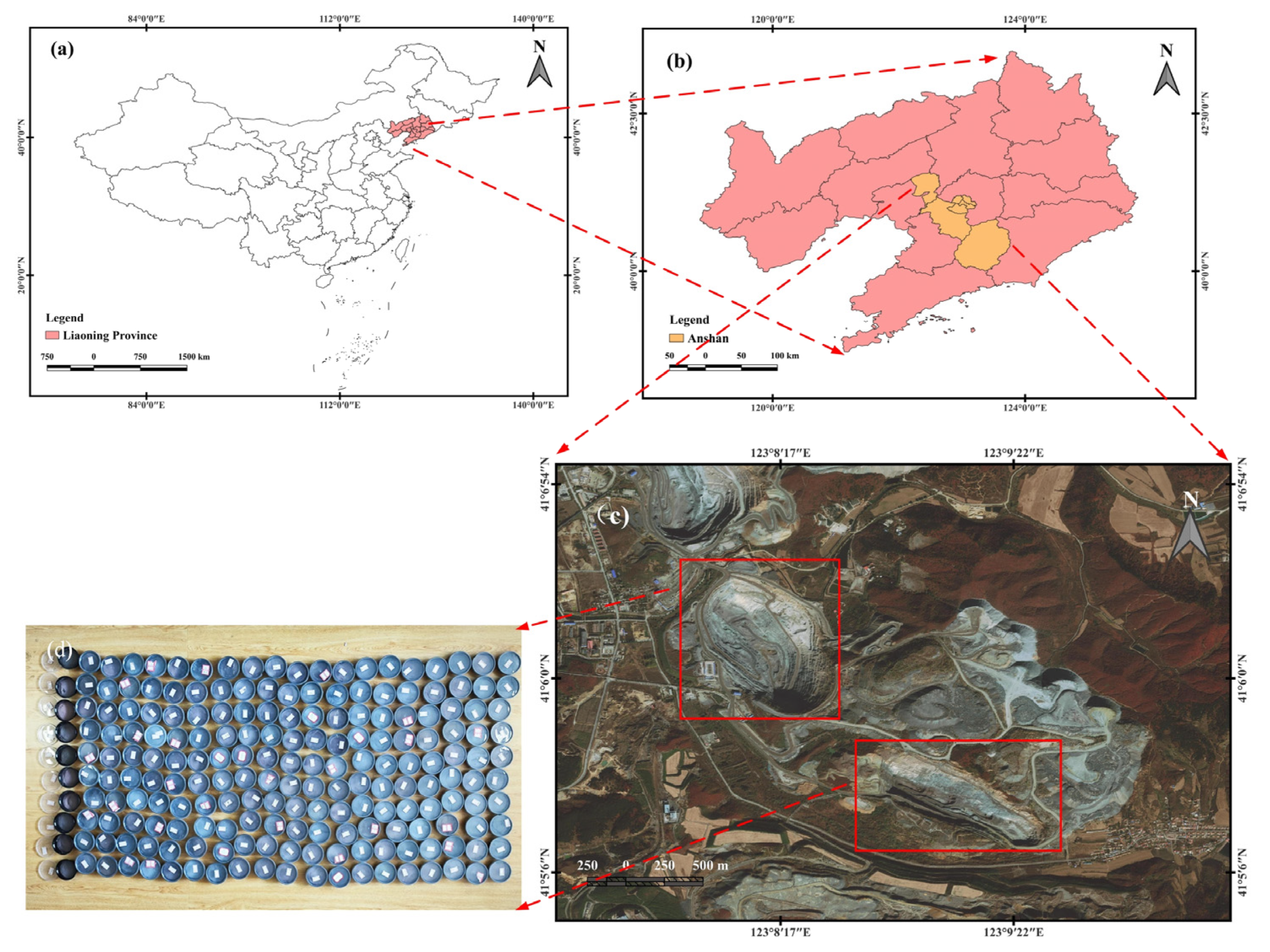
2.1. Study Area

The Anshan area is an important iron ore producing area in China, with its total iron ore resources accounting for about 1/3 of the total iron ore resources in the country. Therefore, this paper takes the Anqian Mine open-pit mine in Anshan City, Liaoning Province, China, as the study area. The geographic coordinates of the mine area are 41°6′32″–41°5′11″ north latitude and 123°7′54″–123°10′5″ east longitude. Figure 1 shows the study area of this paper.

2.2. Spectral Data

In support of this paper, 200 iron ore samples were collected from different locations in the study area. The sample collection date was 18 September 2022. The iron ore samples were processed by crushing, grinding, and sieving to make 200 powdered iron ore samples, and the samples of the processed iron ore are shown in Figure 1. Then, the samples were subjected to spectroscopic experiments using an HR SVC-1024 spectrometer. The band range was 340–2500 nm. After performing five spectral experiments, the TFE of the powder was determined using potassium dichromate titration. (The executive standard of the Potassium dichromate titration method is GB/T 6730.65-2009). The five spectra were averaged as the final sample spectral data. The original spectral curve is shown in Figure 2.

2.3. Remote Sensing Data

The samples were collected using the five-point-sampling method, and the latitude and longitude information of the samples are recorded in this paper to accurately correspond the sample information to the remote sensing information. The sample collection area is shown in Figure 3. Clear and cloudless weather was chosen for collecting samples to avoid excessive cloudiness and water content in the remote sensing information. Sentinel-2 data close to the ore collection date were selected as the remote sensing data. The remote sensing image was taken on 20 September 2022.

Sentinel-2 remote sensing images that have been radiometrically calibrated, geometrically corrected, and atmospherically corrected were downloaded from the ESA website. The remote sensing image contained the mining area of this study. The nearest-neighbor method was used to resample all the bands, and band fusion was performed to obtain color remote sensing images with a resolution of 10 m. Then, the remote sensing image was cropped to obtain the remote sensing image of the study area. The final remote sensing image obtained is shown in Figure 4.

The five-point-sampling method was utilized to obtain the TFE content corresponding to 82 pixel points and to extract the reflectance of 82 pixel points. The reflectance of 82 pixel points is shown in Figure 5.

2.4. Wavelet Transform

The wavelet transform (WT) [34] first transforms the original spectrum to obtain high- and low-frequency wavelet coefficients. Then, the information that is considered to represent noise in the wavelet coefficients is removed. Finally, the processed wavelet coefficients are inversely transformed to obtain smoothed and filtered spectral data.

$${\mathsf{\psi }}_{a,b}=\sqrt{\frac{1}{a}}\mathsf{\psi }(\frac{C-b}{a})$$

(1)

$$W{T}_C(a,b)={\displaystyle {\int }_{-\infty }^{+\infty }x(C)}{\mathsf{\psi }}_{a,b}(C)dC$$

(2)

where a is the scale parameter; b is the translation parameter; $\mathsf{\psi }$ is the wavelet basis function; C is the number of bands; and x(C) is the reflectance at the C band.

2.5. MSSA

SSA, as a swarm intelligence optimization algorithm, has proven its ability to search for optimization [35,36,37]. The position of the i-th sparrow is $X_i=(x_i^1,x_i^2,\mathrm{\dots },x_i^d)$; the fitness value is $f_i=f(x_i^1,x_i^2,\mathrm{\dots },x_i^d)$. Let there be n sparrows in the sparrow population, and the position of each sparrow is d-dimensional.

$$X=\left[\begin{array}{cccc}{x}_1^1& x_1^2& \mathrm{\dots }& x_1^d\\ x_2^1& x_2^2& \mathrm{\dots }& x_2^d\\ \mathrm{\dots }& \mathrm{\dots }& \mathrm{\dots }& \mathrm{\dots }\\ x_n^1& x_n^1& \mathrm{\dots }& x_n^d\end{array}\right].\hspace{1em}{F}_x=\left[\begin{array}{c}f(x_1^1,x_1^2,\mathrm{\dots },x_1^d)\\ \begin{array}{c}f(x_2^1,x_2^2,\mathrm{\dots },x_2^d)\\ \mathrm{\dots }\end{array}\\ f(x_n^1,x_n^2,\mathrm{\dots },x_n^d)\end{array}\right]$$

(3)

In SSA, the discoverers have better fitness values, so they have better search precedence. Therefore, the position of the discoverers is updated as in Equation (4).

$$X_{i,j}^{t+1}=\left\{\begin{array}{c}{X}_{i,d}^t\times \exp (\frac{-i}{\alpha \times ite{r}_{\max }}),R_2<ST\\ X_{i,d}^t+Q\cdot L,R_2\ge ST\end{array}\right.$$

(4)

where iter_max is the maximum search count, j is the solution space, i is the sparrow number, t is the current search count, and $\alpha \in (0,1]$ is a random value. R₂ is a uniformly distributed random value, which represents a warning value, $R_2\in [0,1]$. ST is a random value in [0.5, 1], which represents the sparrow safety value. Q is a value randomly taken in the standard Gaussian distribution, and L is an all-1 matrix.

Equation (5) is the follower’s update method.

$$X_{i,j}^{t+1}=\left\{\begin{array}{c}Q\cdot \exp (\frac{X_{worst} - X_{i,j}^t}{i^2}),i>\frac{n}{2}\\ X_p^{t+1}+\left|X_{i,j}-X_P^{t+1}\right|\cdot A^{+}\cdot L,otherwise\end{array}\right.$$

(5)

$$A^{+}=A^T{(A{A}^T)}^{-1}$$

(6)

where X_P is the best solution space of the current discoverer search, X_worst is the worst solution space of the population, and A is a 1*d-dimensional matrix with random values of 1 or −1.

The position of the alert sparrow is updated according to Equation (7).

$$X_{i,j}^{t+1}=\left\{\begin{array}{c}{X}_{best}^t+\beta \cdot \left|X_{i.j}^t-X_{best}^t\right|, f_i\ne f_g\\ X_{i,j}^t+K\cdot (\frac{\left|X_{i,j}^t - X_{worst}^t\right|}{(f_i - f_w) + \epsilon }), f_i=f_g\end{array}\right.$$

(7)

where X_best is the best solution space for the current population. β is the random number of the control step size, and its value conforms to the standard Gaussian distribution. K is a random value that conforms to a uniform distribution and takes values in the range [−1, 1]. f_i is the i-th individual solution. f_g and f_w are the current optimal solution and the current worst solution, respectively. ε is a constant.

This paper proposes an MSSA by introducing the Lévy flight and a random wandering strategy. Lévy flight is represented by Equation (8).

$$X_i^{\prime }(t)=X_i(t)+\epsilon \cdot rl$$

(8)

where $\epsilon$ controls the step size, and rl represents the Lévy distribution as a random number. The random wandering strategy can increase the diversity of solutions. The random wandering strategy can be represented by Equation (9).

$$X_i^{\prime }(t)=X_i(t)+\delta \cdot (X_j(t)-X_k(t))$$

(9)

where X_j(t) and X_k(t) are the j-th and k-th solution spaces, respectively; $\delta$ represents the scaling factor. The probability P is set to 0.5. When the random number is greater than 0.5, it executes Lévy flight; meanwhile, when the random number is less than 0.5, it executes random wandering.

2.6. VTELM

VTELM is an ML algorithm that extends ELM into two hidden layers. To maintain the diversity of network nodes and enhance the flexibility of the algorithm, VTELM allows each layer to have a different number of nodes. Figure 6 shows the structure of VTELM.

For N samples ${\{X_i,T_i\}}_{i=1}^N$, $X_i={[X_{i1},X_{i2},\cdot \cdot \cdot ,X_{in}]}^T\in R^n$, $T_i=[T_{i1},T_{i2},\cdot \cdot \cdot ,T_{im}]\in R^m$, n is the number of input features, and m is the number of output features. L₁ and L₂ represent the number of nodes in the first and second hidden layers, respectively, and the node parameters are randomly valued. The weights W₁ and W₂ have a value range of [−1, 1], and the thresholds B₁ and B₂ have a value range of [0, 1]. Given the activation function g, the output matrix H₁ of the first hidden layer is calculated according to Equation (10).

$$H_1=g(W_{1}X+B_1)$$

(10)

H₁ is used as input to calculate the network output H₂ of the next layer.

$$H_2=g(W_2{H}_1+B_2)$$

(11)

The $\beta$ can be solved by Equation (12).

$$\stackrel{\wedge }{\beta }=H_2^{+}T$$

(12)

where $H_2^{+}$ is the Moore–Penrose generalized inverse matrix of $H_2$. The final output of the VTELM algorithm is expressed by Equation (13).

$$f(x)=g(W_{2}g(W_{1}X+B_1)+B_2)\beta$$

(13)

2.7. MSSA-BNVTELM

The VTELM algorithm needs to use twice the activation function to express the nonlinearity of the algorithm. The activation function can improve the nonlinearity and generalization of the algorithm. However, the activation functions used by the VTELM algorithm all have a saturation region. If g enters the saturation region, the output becomes insensitive to small differences in the inputs. At this time, even though the input features vary a lot, the output features vary only a small amount. This results in the differences between the input features being heavily scaled down. Therefore, when g enters the saturation region, the output features cannot reflect the changes of the input features.

Observing Figure 7, these three activation functions exist in their respective saturation regions. When the independent variable is greater than 4, it is obvious that the sigmoid and dsig functions enter the saturation region, at which point the output becomes insensitive to minor variations in the input. When the independent variable is greater than 2, the tanh function enters the saturation region. To solve the activation function saturation problem, the BN structure is introduced in this paper before calculating the activation function. Figure 8 shows the structure of BNVTELM.

After adding BN, the net output h₁ of the first layer network is calculated according to Equation (14).

$$h_1=W_{1}X+B_1$$

(14)

After transforming the net output h₁ into a standard normal distribution, H₁ is calculated according to Equation (15).

$$H_1=g(\frac{h_1-E[h_1]}{\sqrt{Var[h_1]}})$$

(15)

where Var[h₁] denotes the variance of h₁, and E[h₁] denotes the mean value of h₁. The net output of the second layer network is calculated according to Equation (16).

$$h_2=W_2{H}_1+B_2$$

(16)

H₂ is calculated according to Equation (17).

$$H_2=g(\frac{h_2-E[h_2]}{\sqrt{Var[h_2]}})$$

(17)

The $\beta$ is still calculated according to Equation (12). The final output of BNVTELM is expressed by Equation (18), where Z in Equation (18) represents the calculation process of transforming the net output into a standard normal distribution.

$$f(X)=g(Z(W_{2}g(Z(W_{1}X+B_1))+B_2))\beta$$

(18)

In updating the BNVTELM parameters using MSSA, the total number of parameters is used as the dimension of the solution. The root mean square error (RMSE) is used as the fitness value. The MSSA-BNVTELM training process is recorded in Algorithm 1. The RMSE is calculated as follows:

$$\mathrm{RMSE}=\sqrt{{\displaystyle \sum _{i=1}^N(Y_i-Y_i^{*})/N}}$$

(19)

where Y denotes the actual value, and Y^* denotes the calculated value.

Algorithm 1 The algorithm flow of MSSA-BNVTELM
1	W1, W2, B1, and B2 are initialized randomly as sparrow positions.
2	Set MSSA parameters, population size, number of iterations, expectation error e, etc.
3	The $\beta$ is solved according to Equation (12).
4	Calculate the fitness value of each sparrow according to Equation (19).
5	Update the discoverer location according to Equation (4).
6	The follower position is updated according to Equation (5).
7	Update the vigilante position according to Equation (7).
8	Performs random wandering or Lévy flight with probability 0.5.
9	Recalculate $\beta$ for the updated individuals
10	Calculate RMSE according to Equation (19). If RMSE < e, the update is stopped; otherwise, return to step 5. The algorithm also stops updating if the number of iterations reaches the set requirement.

2.8. Uncertainty Analysis

In order to ensure the availability of the TFE detection model, the uncertainty of the model must be analyzed [38]. In this paper, the uncertainty of the TFE detection model is analyzed using a bootstrapping technique [39]. In each iteration of bootstrapping uncertainty analysis, 75% of the samples are randomly selected as training set samples, and 25% of the samples are randomly selected as test set samples to train 50 different MSSA-BNVTELM models. Then, we calculate the detection indexes based on test set outputs versus actual outputs.

3. Results and Discussion

3.1. WT and Feature Extraction

In WT, the dblets wavelets are chosen as wavelet basis functions for the analysis. To determine the number of decomposition layers of the dblets wavelet basis, db2, db3, db4, db5, and db6 are used to process the visible—infrared spectral data. To evaluate the noise-filtering effect, this paper uses the linear regression method to model and analyze the spectra after WT and uses RMSE as an evaluation index. When the RMSE is smaller, it proves that the linear regression fit is better, and the de-noising effect is better. In this paper, the spectral signals are processed using db2, db3, db4, db5, and db6 with decomposition levels from 2 to 8.

Observing Figure 9, the curves show a decreasing and then increasing trend. When the decomposition level is greater than 3, the distinction of the curve is small. The RMSE of the db4 wavelet reaches its minimum when the decomposition level is 4. Therefore, in this paper, the db4 wavelet with a decomposition level of 4 is chosen to denoise the spectrum. Figure 10 shows the spectra after denoising. Comparing to Figure 2, we can see that the curve in Figure 10 is smoother, which indicates that WT removes some noise from the spectrum.

The spectral experiments are conducted in the band range of 340–2500 nm, and the visible—infrared spectral data are 973 dimensions. The three-dimensional data at 340 and 2500 are removed because of the high noise contamination of the spectral data at these two bands. However, the 970-dimensional data have the problems of information redundancy and multicollinearity. If the 970-dimensional data are used as input, the accuracy of the algorithm will be reduced. Moreover, to match the high-dimensional input features, ELM needs to set a large number of hidden layer nodes, which will cause a redundant network structure and reduce the generalizability of ELM. Therefore, this paper uses PCA to reduce the dimensionality of 970-dimensional data. In this paper, the cumulative contribution rate is set to 99.9%, and six-dimensional features are extracted. The extracted features are shown in Figure 11. These six-dimensional features will be used as input features for subsequent iron ore detection model building.

3.2. Comparison of MSSA and SSA

In order to test whether the random wandering strategy with Lévy flight can improve the global search ability of SSA, this paper compares SSA-ELM with MSSA-ELM and records the results in Figure 12. All parameters are set identically in the comparison experiments. The W and B of ELM are the positions of sparrows, and RMSE is the fitness value. The number of iterations (t) and the number of populations (pop) are 30 and 40, respectively, and predators account for 20% of the pop.

In Figure 12, it can be clearly seen that both SSA-ELM and MSSA-ELM have decreasing RMSE as t increases. This shows that both SSA and MSSA can optimize ELM parameters and improve the prediction accuracy of ELM. When t is 2, the RMSE of MSSA-ELM begins to decrease until it reaches its minimum value at t of 7. However, when t is 12, the RMSE of SSA-ELM begins to decrease until it reaches its minimum value at t of 17. Therefore, MSSA-ELM has faster convergence than SSA-ELM. The best RMSE for MSSA-ELM is 2.764 compared with 2.849 for SSA-ELM; therefore, MSSA has better search capability than SSA. Therefore, the random wandering strategy and Lévy flight can increase the global search capability and speed up the convergence of SSA.

3.3. Hidden Layer Node Testing

Compared with ELM, VTELM increases the depth of the network. Therefore, VTELM needs to set the number of the two hidden layer nodes because the parameters between the two hidden layers are randomly generated. If the number of nodes does not match the scale of the model, it will cause a decrease in VTELM accuracy. Therefore, in this paper, the number of hidden layer nodes in VTELM is tested to determine the optimal number of nodes, using RMSE as the evaluation index. In order to expand the search range, the first layer nodes (L₁) are set to 5 to 40, and the second layer nodes (L₂) are set to 5 to 50 in this paper. After simulation experiments, the variation law of VTELM accuracy with the change of the number of nodes is obtained.

Observing Figure 13, the error generated by the algorithm is mainly controlled by L₂. The RMSE increases significantly when L₂ is greater than 30. When L₂ is approximately 30, RMSE decreases significantly compared to other L₂ values. When L₂ remains constant, RMSE decreases as L₁ increases. Therefore, we set L₁ and L₂ to be 20 and 30, respectively.

3.4. Model Comparison

In this paper, MSSA-BNVTELM, back propagation neural network (BP), radial basis function (RBF), and other algorithms are used to build a TFE detection model. All models use the same data, and the RMSE, mean absolute error (MAE), ratio of performance to interquartile (RPIQ), and Pearson coefficient (R²) are used as evaluation metrics to evaluate the accuracy of the models. Equations (20)–(22) are the computing methods for MAE, RPIQ, and R², respectively. To avoid the uncertainty of a single test, five experiments are conducted in this paper, and the average results of the five experiments are recorded in

Table 1. Algorithm Comparison.

Algorithm	RMSE	R2	MAE	RPIQ
BP	4.325	0.745	3.180	1.245
RBF	3.731	0.786	2.716	1.264
ELM	3.392	0.802	2.627	1.306
VTELM	3.175	0.828	2.312	1.392
MSSA-BNVTELM	2.164	0.943	1.702	1.521

.

$$\mathrm{MAE}=\frac{{\displaystyle \sum _{i=1}^N\left|Y_i-Y_i^{*}\right|}}{N}$$

(20)

$$\mathrm{RPIQ}=\frac{Q_3-Q_1}{\sqrt{\mathrm{RMSE}}}$$

(21)

$${\mathrm{R}}^2=\frac{N{\displaystyle \sum _{i=1}^N{Y}_i}{Y}_i^{*}-{\displaystyle \sum _{i=1}^N{Y}_i^{*}}{\displaystyle \sum _{i=1}^N{Y}_i}}{\sqrt{N{\displaystyle \sum _{i=1}^N{(Y_i^{*})}^2-({\displaystyle \sum _{i=1}^N{Y}_i^{*}{)}^2}}}\sqrt{N{\displaystyle \sum _{i=1}^N{(Y_i)}^2-({\displaystyle \sum _{i=1}^N{Y}_i^{*}{)}^2}}}}$$

(22)

where Y, Y^*, and N have the same meaning as Y, Y^*, and N in Equation (19). Q₃ and Q₁ are, respectively, values located at 75% size and 25% size.

Firstly, RBF obtains higher detection accuracy than BP from the experimental results. BP requires a gradient descent method to update the parameters, and it is easy to fall into the problem of local minima that cannot be avoided fundamentally; therefore, the stability of BP is low. However, RBF solves the problem of local minima from the computational method, so the detection accuracy of RBF gains improvement. However, RBF requires a large number of hyperparameters to be set, which leads to poor detection generalization of RBF. Comparing RBF and BP, ELM not only solves the local minimum problem but also requires only one parameter setting to complete the training of the algorithm, which reduces the dependence of ELM on parameter setting. Therefore, according to the information in Table 1, ELM has higher detection accuracy than BP and RBF. This shows that ELM can detect the TFE more accurately than BP and RBF. The accuracy of VTELM is improved compared to ELM by increasing the number of hidden layers and changing the solving relationship of parameters between two hidden layers. Compared with VTELM, the detection accuracy of MSSA-BNVTELM is further improved, which indicates that the improvement of VTELM using MSSA and BN can increase the detection accuracy of VTELM. In addition, MSSA-BNVTELM has the highest detection accuracy among these five algorithms. Therefore, the MSSA-BNVTELM proposed in this paper can detect the TFE more accurately compared with other algorithms.

In order to show more intuitively whether the output results of MSSA-BNVTELM can approximate the test set outputs, this paper plots the comparison between the experimental results and the actual values. The comparison results are shown in Figure 14. Observing Figure 14, it can be seen that the outputs of MSSA-BNVTELM can all be well approximated to the actual values, which indicates that TFE in ore can be effectively and accurately detected in this paper by utilizing MSSA-BNVTELM combined with visible—infrared spectroscopy.

3.5. Remote Sensing Detection

In order to detect the TFE content of the whole mining area, the reflectances corresponding to 82 pixel points are used as samples, and MSSA-BNVTELM, VTELM, ELM, BP, and RBF are used as modeling methods to model and analyze the mining area. The reflectances corresponding to 62 pixel points were used to train the algorithms, and the reflectances corresponding to 20 pixel points were used to test the algorithms. In order to select the appropriate remote sensing data, in this paper, Landsat-8 data and Sentinel-2 data were used for modeling.

Table 2. Remote sensing test comparison (Sentinel-2 data).

Algorithm	RMSE	R2	MAE	RPIQ
BP	3.052	0.744	2.622	0.989
RBF	3.229	0.685	2.775	0.905
ELM	2.685	0.889	2.374	1.101
VTELM	2.128	0.905	1.782	1.305
MSSA-BNVTELM	1.358	0.962	1.116	1.337

shows the test results using Sentinel-2 data.

Table 3. Remote sensing test comparison (Landsat-8 data).

Algorithm	RMSE	R2	MAE	RPIQ
BP	3.018	0.794	2.453	1.052
RBF	3.742	0.581	3.274	1.143
ELM	2.976	0.851	2.431	1.221
VTELM	2.201	0.881	1.834	1.155
MSSA-BNVTELM	1.647	0.923	1.245	1.317

shows the test results using Landsat-8 data.

The characteristic of ELM using the least-squares method to train network parameters ensures its high generalization and can adapt to more data learning. Therefore, the detection accuracy of ELM is higher than that of BP and RBF. The increase in network depth ensures that the detection accuracy of VTELM is higher than that of ELM. In order to further improve the detection accuracy of VTELM algorithm, this paper uses BN and MSSA to improve and optimize the network structure and parameters of VTELM. MSSA-BNVTELM has the highest detection accuracy compared to other mine detection models both using Landsat-8 data and Sentinel-2 data. This indicates that the improved approach of BN with MSSA not only makes MSSA-BNVTEM perform well in spectral data but also achieve success in remote sensing detection. MSSA and BN can improve the generalization and detection accuracy of VTELM. Observing the BP, the detection accuracy in using Landsat-8 data is higher than the detection accuracy in using Sentinel-2. The reduction of input data features causes the number of parameters that need to be updated by gradient descent in the BP algorithm to decrease and also reduces the possibility of locally optimal solutions. When modeling with Sentinel-2 data, the increase in input features requires more hidden layer nodes to be matched, so the amount of parameters becomes larger, and the possibility of falling into local optimal solutions increases.

However, it should be noted that modeling with Sentinel-2 data may be more appropriate for detecting TFE at the mine site than using Landsat-8 data. All models except BP had significantly higher accuracy when modeled with Sentinel-2 data than with Landsat-8 data. And from the final experimental data, it can be seen that MSSA-BNVTELM has the highest detection accuracy when modeled with Sentinel-2 data, with an R² of 0.962 and an RMSE of 1.358. Compared to the 7-band data of Landsat-8, Sentinel-2 data has 11-band data, so Sentinel-2 can provide more spectral information and is more suitable for detecting TEF.

In order to visualize the TFE content of the whole mine, this paper extracts the reflectance of all the pixel points in Figure 4. The reflectance was taken as input, and the trained MSSA-BNVTELM was used as a detection model to predict the TFE in the mine area, and the prediction was plotted. The TFE distribution of the mine area is shown in Figure 15. According to Figure 15, the distribution of TFE in the mine area can be clearly seen, which can be helpful for the development of the mine’s mining plan.

3.6. Uncertainty Analysis of Detection Models

The uncertainty of the TFE detection model must be quantified to ensure the stability of the detection model. This quantification of uncertainty can be assessed by comparing the metrics obtained from cross-validation with the metrics obtained using bootstrapping technique. The uncertainty of the TFE detection model is calculated based on 50 bootstrapping iterations, and the results are shown in

Table 4. TFE detection model (MSSA-BNVTELM) metrics with 50 bootstrap iterations.

Input Data	RMSE	R2	MAE	RPIQ
Visible–infrared	2.089	0.941	1.588	1.623
Sentinel-2	1.180	0.958	1.008	1.452
Landsat-8	1.752	0.938	1.227	1.511

Compared to the cross-validation models (Table 1, Table 2 and Table 3), the fitting metrics of the bootstrap method (Table 4) show less variation in the metrics of the MSSA-BNVTELM model, which indicates that the MSSA-BNVTELM builds a model with lower variability and uncertainty. For example, when the input data are from Sentinel-2, the MAE of the cross-validated model is 1.116, while the bootstrap uncertainty result produces an MAE of 1.008, which is a smaller deviation.

4. Conclusions

Rapid detection of TFE can accelerate iron ore production. Restricted by the efficiency of chemical testing methods, it is difficult to achieve a quantitative analysis of each ore in mine production. As a result, ore blending has the problem of low efficiency and inaccuracy. This paper proposes visible—infrared spectroscopy combined with a machine learning detection method to improve the detection efficiency of TFE. First, we measured the visible—infrared spectrum of iron ore using an HR SVC-1024 spectrometer. In order to reduce the error caused by a single measurement, the spectral experiment was executed five times, and then, the average value was taken as the visible—infrared spectrum of the sample. Then, the spectra were smoothed and filtered based on the WT. The PCA was used to extract spectral features because of the large dimensionality of the original spectra. Finally, the ELM was optimized using SSA to improve its stability and accuracy. In this paper, two strategies were used to modify SSA to further improve its optimization capability. The experiments proved that MSSA has a stronger global search capability than SSA. Therefore, this paper uses MSSA to optimize the VTELM parameters. In addition, in order to maintain the sensitivity of the activation function, this paper adds BN structure to the VTELM algorithm and proposes an MSSA-BNVTELM algorithm. The experiments proved that MSSA-BNVTELM can detect the TFE of iron ore accurately and quickly. This paper presents a novel method for the rapid detection of TFE, which is important for accelerating iron ore production and improving production efficiency.

In addition, this paper utilizes Sentinel-2 and Landsat-8 data to establish TFE detection models in the mining area. According to the comparison of the experimental results, it was found that Sentinel-2 data are more suitable for detecting TFE content. The R² of the model established by Sentinel-2 is 0.96, and the R² of the model established by Landsat-8 is 0.96. Finally, the reflectance of all pixel points of the Sentinel-2 remote sensing image was extracted and inputted into the trained model to obtain the TFE distribution map of the mine site. The TFE distribution map clearly shows the distribution of TFE at the mine site, which can help in the production planning of the mine.

References

1. Yao, J.; Liu, C.; Huang, G.; Xu, K.; Yuan, Q. Multi-Source and Multi-Target Iron Ore Blending Method in Open Pit Mine. Arch. Min. Sci. 2022, 67, 631–644. [Google Scholar]
2. Cao, Y.; Wu, S.; Han, H.; Wang, H.; Xue, F.; Liu, X. Mixed State and High Effective Utilization of Pilbara Blending Iron Ore Powder. J. Iron Steel Res. Int. 2011, 18, 1–5. [Google Scholar] [CrossRef]
3. Cheng, Y.; Shen, Z.; Yang, Y.; Liang, Q.; Liu, H. Development of a Redox Microtitration Method for the Determination of Metallic Iron Content in Reduced Micron-Sized Iron Ore Concentrate Particles. Metall. Mater. Trans. B-Proc. Metall. Mater. Proc. Sci. 2022, 53, 807–815. [Google Scholar] [CrossRef]
4. Hu, H.; Tang, Y.; Ying, H.; Wang, M.; Wan, P.; Yang, X.J. The Effect of Copper on Iron Reduction and Its Application to the Determination of Total Iron Content in Iron and Copper Ores by Potassium Dichromate Titration. Talanta 2014, 125, 425–431. [Google Scholar] [CrossRef] [PubMed]
5. Xie, H.; Mao, Z.; Xiao, D.; Liu, J. Rapid Detection of Copper Ore Grade Based on Visible-Infrared Spectroscopy and TSVD-IVTELM. Measurement 2022, 203, 112003. [Google Scholar] [CrossRef]
6. Singh, N.; Rashmi; Gupta, P.K. Measurements of major and minor constituents in sulphide ore by gravimetry followed by flame atomic absorption spectrometry. Rev. Anal. Chem. 2006, 25, 141–153. [Google Scholar] [CrossRef]
7. Guatame-Garcia, A.; Buxton, M. The Use of Infrared Spectroscopy to Determine the Quality of Carbonate-Rich Diatomite Ores. Minerals 2018, 8, 120. [Google Scholar] [CrossRef]
8. Prado, E.M.G.; Silva, A.M.; Ducart, D.F.; Toledo, C.L.B.; de Assis, L.M. Reflectance Spectroradiometry Applied to a Semi-Quantitative Analysis of the Mineralogy of the N4ws Deposit, Carajás Mineral Province, Pará, Brazil. Ore Geol. Rev. 2016, 78, 101–119. [Google Scholar] [CrossRef]
9. Oluwaseye, F.I.; Iyakwari, S.; Idzi, A.A.; Kehinde, O.H.; Osu, U. Qualitative identification of copper bearing minerals using near infrared sensors. Physicochem. Probl. Miner. Process. 2016, 52, 620–633. [Google Scholar]
10. Basile, A.; Hughes, J.; McFarlane, A.J.; Bhargava, S.K. Development of a Model for Serpentine Quantification in Nickel Laterite Minerals by Infrared Spectroscopy. Miner. Eng. 2010, 23, 407–412. [Google Scholar] [CrossRef]
11. Li, W.J.; Pang, J.M. Application of Remote Sensing in Investigation of Geological Environment of Iron Mine. In Proceedings of the 2020 5th International Conference on Materials Science, Energy Technology and Environmental Engineering, Shanghai, China, 7–9 August 2020; Volume 571, p. 012079. [Google Scholar]
12. Hai, W.J.; Xia, N.; Song, J.M.; Tang, M.Y. Identification and Monitoring of Surface Elements in Open-Pit Coal Mine Area Based on Multi-Source Remote Sensing Images. Pol. J. Environ. Stud. 2022, 31, 4127–4136. [Google Scholar] [CrossRef]
13. Ali, N.; Fu, X.D.; Ashraf, U.; Chen, J.; Thanh, H.V.; Anees, A.; Riaz, M.S.; Fida, M.; Hussain, M.A.; Hussain, S.; et al. Remote Sensing for Surface Coal Mining and Reclamation Monitoring in the Central Salt Range, Punjab, Pakistan. Sustainability 2022, 14, 9835. [Google Scholar] [CrossRef]
14. Li, H.K.; Xu, F.; Weng, X.Y. Recognition method for high-resolution remote-sensing imageries of ionic rare earth mining based on object-oriented technology. Arab. J. Geosci. 2020, 13, 1137. [Google Scholar] [CrossRef]
15. Xiao, D.; Xie, H.; Fu, Y.; Li, F. Inversion of Low-Grade Copper Mining Areas Based on Spectral Information and Remote Sensing Data Using Vis-NIR. Spectroscopy 2022, 36, 30–37. [Google Scholar]
16. Xiao, D.; Xie, H.; Fu, Y.; Li, F. Mine Reclamation Based on Remote Sensing Information and Error Compensation Extreme Learning Machine. Spectrosc. Lett. 2021, 54, 151–164. [Google Scholar] [CrossRef]
17. Le, B.T.; Xiao, D.; Okello, D.; He, D.; Xu, J.; Doan, T.T. Coal Exploration Technology Based on Visible-Infrared Spectra and Remote Sensing Data. Spectrosc. Lett. 2017, 50, 440–450. [Google Scholar] [CrossRef]
18. Ju, H.; Bi, F.; Bian, M.; Shi, Y. Multiscale Feature Fusion Network for Automatic Port Segmentation from Remote Sensing Images. J. Appl. Remote Sens. 2022, 16, 044506. [Google Scholar] [CrossRef]
19. Chen, Y.N.; Fan, K.C.; Chang, Y.L.; Moriyama, T. Special Issue Review: Artificial Intelligence and Machine Learning Applications in Remote Sensing. Remote Sens. 2023, 15, 569. [Google Scholar] [CrossRef]
20. Xu, S.; Deng, B.; Meng, Y.; Liu, G.; Han, J. ReA-Net: A Multiscale Region Attention Network With Neighborhood Consistency Supervision for Building Extraction From Remote Sensing Image. IEEE J. Sel. Top. Appl. Earth Obs. Remote Sens. 2022, 15, 9033–9047. [Google Scholar] [CrossRef]
21. Huang, G.B.; Zhou, H.; Ding, X.; Zhang, R. Extreme Learning Machine for Regression and Multiclass Classification. IEEE Trans. Syst. Man Cybern. Part B-Cybern. 2012, 42, 513–529. [Google Scholar] [CrossRef]
22. Huang, G.B.; Zhu, Q.Y.; Siew, C.K. Extreme Learning Machine: Theory and Applications. Neurocomputing 2006, 70, 489–501. [Google Scholar] [CrossRef]
23. Cao, J.; Lin, Z. Extreme Learning Machines on High Dimensional and Large Data Applications: A Survey. Math. Probl. Eng. 2015, 2015, 103796. [Google Scholar] [CrossRef]
24. Xiao, D.; Huang, J.; Li, J.; Fu, Y.; Li, Z. Inversion Study of Cadmium Content in Soil Based on Reflection Spectroscopy and MSC-ELM Model. Spectrochim. Acta Part A Mol. Biomol. Spectrosc. 2022, 283, 121696. [Google Scholar] [CrossRef] [PubMed]
25. Li, R.; Huang, W.; Shang, G.; Zhang, X.; Wang, X.; Liu, J.; Wang, Y.; Qiao, J.; Fan, X.; Wu, K.; et al. Rapid Recognizing the Producing Area of a Tobacco Leaf Using Near-Infrared Technology and a Multi-Layer Extreme Learning Machine Algorithm. J. Braz. Chem. Soc. 2022, 33, 251–259. [Google Scholar] [CrossRef]
26. Li, R.; Zhang, X.; Li, K.; Qiao, J.; Wang, Y.; Zhang, J.; Zi, W. Nondestructive and Rapid Grading of Tobacco Leaves by Use of a Hand-Held near-Infrared Spectrometer, Based on a Particle Swarm Optimization-Extreme Learning Machine Algorithm. Spectrosc. Lett. 2020, 53, 685–691. [Google Scholar] [CrossRef]
27. Zheng, W.; Fu, X.; Ying, Y. Spectroscopy-Based Food Classification with Extreme Learning Machine. Chemom. Intell. Lab. Syst. 2014, 139, 42–47. [Google Scholar] [CrossRef]
28. Yin, H.; Chen, C.; He, Y.; Jia, J.; Chen, Y.; Du, R.; Xiang, R.; Zhang, X.; Zhang, Z. Synergistic Estimation of Soil Salinity Based on Sentinel-1 Image Texture and Sentinel-2 Salinity Spectral Indices. J. Appl. Remote Sens. 2023, 17, 018502. [Google Scholar] [CrossRef]
29. Yan, D.; Chu, Y.; Li, L.; Liu, D. Hyperspectral Remote Sensing Image Classification with Information Discriminative Extreme Learning Machine. Multimed. Tools Appl. 2018, 77, 5803–5818. [Google Scholar] [CrossRef]
30. Liang, X.J.; Qin, P.; Xiao, Y.F.; Kim, K.Y.; Liu, R.J.; Chen, X.Y.; Wang, Q.B. Automatic Remote Sensing Detection of Floating Macroalgae in the Yellow and East China Seas Using Extreme Learning Machine. J. Coast. Res. 2019, 90, 272–281. [Google Scholar] [CrossRef]
31. Fu, Y.; Xie, H.; Mao, Y.; Ren, T.; Xiao, D. Copper Content Inversion of Copper Ore Based on Reflectance Spectra and the VTELM Algorithm. Sensors 2020, 20, 6780. [Google Scholar] [CrossRef]
32. Xue, J.; Shen, B. A Novel Swarm Intelligence Optimization Approach: Sparrow Search Algorithm. Syst. Sci. Control Eng. 2020, 8, 22–34. [Google Scholar] [CrossRef]
33. Ioffe, S.; Szegedy, C. Batch Normalization: Accelerating Deep Network Training by Reducing Internal Covariate Shift. In Proceedings of the 32nd International Conference on Machine Learning (PMLR), Lille, France, 7–9 July 2015; Volume 37, pp. 448–456. [Google Scholar]
34. Zhou, F.; Zhu, H.; Li, C. A Pretreatment Method Based on Wavelet Transform for Quantitative Analysis of UV–Vis Spectroscopy. Optik 2019, 182, 786–792. [Google Scholar] [CrossRef]
35. Zhang, C.; Chen, P.; Jiang, F.; Xie, J.; Yu, T. Fault Diagnosis of Nuclear Power Plant Based on Sparrow Search Algorithm Optimized CNN-LSTM Neural Network. Energies 2023, 16, 2934. [Google Scholar] [CrossRef]
36. Salim, A.; Khedr, A.M.; Osamy, W. IoVSSA: Efficient Mobility-Aware Clustering Algorithm in Internet of Vehicles Using Sparrow Search Algorithm. IEEE Sens. J. 2023, 23, 4239–4255. [Google Scholar] [CrossRef]
37. Ouyang, M.; Wang, Y.; Wu, F.; Lin, Y. Continuous Reactor Temperature Control with Optimized PID Parameters Based on Improved Sparrow Algorithm. Processes 2023, 11, 1302. [Google Scholar] [CrossRef]
38. Gasmi, A.; Gomez, C.; Chehbouni, A.; Dhiba, D.; El Gharous, M. Using PRISMA Hyperspectral Satellite Imagery and GIS Approaches for Soil Fertility Mapping (FertiMap) in Northern Morocco. Remote Sens. 2022, 14, 4080. [Google Scholar] [CrossRef]
39. Breiman, L. Bagging Predictors. Mach. Learn. 1996, 24, 123–140. [Google Scholar] [CrossRef]
Figure 1. Study area. (a) Province in which the study area is located, (b) The city in which the study area is located, (c) The study area of this paper (The red square boxes show the main source areas of the samples), (d) 200 iron ore samples collected from the mining area.
Remotesensing 15 04100 g001
Figure 2. Original spectral curve.
Remotesensing 15 04100 g002
Figure 3. Sample points for the five-point-sampling method.
Remotesensing 15 04100 g003
Figure 4. Sentinel-2 remote sensing images of the study area.
Remotesensing 15 04100 g004
Figure 5. Spectral curves of remote sensing images.
Remotesensing 15 04100 g005
Figure 6. Structure diagram of VTELM.
Remotesensing 15 04100 g006
Figure 7. Curve of activation function.
Remotesensing 15 04100 g007
Figure 8. Curve of activation function.
Remotesensing 15 04100 g008
Figure 9. The effect of different db wavelet denoising.
Remotesensing 15 04100 g009
Figure 10. Spectra after wavelet transform.
Remotesensing 15 04100 g010
Figure 11. PCA extracted spectral features.
Remotesensing 15 04100 g011
Figure 12. Variation of the fitness values with the number of iterations.
Remotesensing 15 04100 g012
Figure 13. Change of RMSE when the number of nodes changes.
Remotesensing 15 04100 g013
Figure 14. Comparison between the best predicted results and actual output.
Remotesensing 15 04100 g014
Figure 15. Comparison between the best predicted results and actual output.
Remotesensing 15 04100 g015