Robust Space-Time Adaptive Processing Method for GNSS Receivers in Coherent Signal Environments

Abstract

In the coherent signal environments caused by multipath propagation, the interference suppression performance of the global navigation satellite systems (GNSS) receivers decreases sharply. In this paper, a robust space-time adaptive processing (STAP) method for GNSS receivers is proposed to suppress interferences in coherent signal environments, by using the modified space-time two-dimensional iterative adaptive approach (ST2D-IAA) spectrum estimation. This method applies the IAA algorithm to the ST2D signal model of GNSS receivers, and further modifies the ST2D-IAA algorithm to accurately estimate the power spectrum and noise power simultaneously. The space-time interference-plus-noise covariance matrix (STINCM) is reconstructed by using the estimated power spectrum and noise power in the interference angle region. Based on the reconstructed STINCM, we construct the STAP beamforming optimization problem for the space-time steering vector (STSV) error vector, and further correct the STSV of GNSS signal. Finally, the weight vector of STAP beamforming is calculated by using the reconstructed STINCM and the corrected STSV of GNSS signal. Simulation results show that the proposed method can suppress interferences in coherent signal environments and outperforms the current methods.

1. Introduction

The global navigation satellite systems (GNSS) use the advantages of satellites to provide real-time, high-precision navigation, positioning and timing services, which play a vital role in the economic and military fields [1,2,3]. The current GNSS mainly includes the United States global positioning systems (GPS), China’s Beidou Systems, Europe’s GALILEO systems and Russia’s GLONASS systems. However, the accuracy and reliability of GNSS receivers can be easily affected by all kinds of intentional and unintentional interferences [4]. With the significant increase in the types and quantities of interference, GNSS applications have posed a great threat, especially the rapid increase in cheap jamming devices [5]. Therefore, it is urgent to improve the interference suppression ability of GNSS receivers. An effective method to suppress interferences is to use antenna array processing technology, which can form a nulling in the direction of interference [6].

A large number of interference suppression algorithms for GNSS receivers based on antenna arrays have been proposed. Among these algorithms, space only processing (SOP) and space-time adaptive processing (STAP) are two typical representatives [7]. The SOP algorithms [8] use only one spatial filter to process the observed signals, mainly divided into power inversion algorithms and adaptive beamforming algorithms. The power inversion algorithms [9] do not need to know the array structure and satellite signal information in advance, and utilizes the characteristics that the intensity of the satellite signal is lower than the noise and interferences when it reaches the receivers. However, this kind of algorithms cannot guarantee that the mainlobe of the beampattern always points to the satellite signal. Adaptive beamforming algorithms are proposed to enhance desired satellite signals while suppressing interference signals which are based on the criteria of minimum variance distortionless response (MVDR), minimum power distortionless response (MPDR) and maximum signal-to-interference-plus-noise ratio (SINR). In practice, there may be direction errors, local scattering, wavefront distortion and limited number of sampling snapshots, which lead to the covariance matrix mismatches and steering vector errors. In order to improve the beamforming performance, a large number of robust adaptive beamforming methods have been proposed to eliminate these errors, such as diagonal loading [10], eigenspace-based [11], uncertainty set-based [12], interference-plus-noise covariance matrix (INCM) reconstruction [13,14,15,16] methods. Although these SOP algorithms can effectively suppress multiple interferences, the degrees-of-freedom of interference suppression is limited by the number of antenna array elements.

In order to overcome the shortcomings of the SOP algorithms, the STAP algorithms are proposed to increase the number of interference suppression degrees-of-freedom in GNSS receivers. The STAP algorithms work by placing a finite impulse response (FIR) filter behind each sensor without the need to increase the number of physical array antennas [17,18,19]. The distortionless STAP method can guarantee the distortionless response of GNSS signal and suppress the interference signals [20]. The essence of this method is to ensure the linearity of the phase by constraining the coefficients of the FIR filter. However, the imprecise prior information caused by the direction errors will result in the mismatch of the steering vector, which further deteriorates the performance of STAP method [21]. Therefore, it is of great significance to study a robust STAP method that can deal with steering vector errors. In the vicinity of GNSS receivers, due to the obstruction of buildings or obstacles, GNSS signal will be refracted and reflected, resulting in the coherent interference, which seriously reduces the positioning performance of GNSS receivers [22].

The multipath signal can be used for remote sensing purposes in GNSS interferometric reflectometry, such as the estimation of lake ice thickness in [23]. In general, the GNSS multipath signal is coherent with the direct line-of-sight signal. As a result, the coherent interference causes the spatial spectrum diffusion in the angle region, which reduces the accuracy of the angle estimation algorithms. In order to deal with the coherent interference problems, the spatial smoothing technique [24] resorves the correlation by restoring the rank of the signal covariance matrix. Forward/backward spatial smoothing techniques [25] construct an average forward/backward covariance matrix by dividing the uniform linear array into multiple coincident subarrays, thereby overcoming the defect of rank deficiency. However, this kind of techniques deal with the coherence problems at the cost of the number of effective degrees-of-freedom, and still cannot deal with the coherent interference completely in the low signal-to-noise ratios (SNR) environments. Since the parametric maximum likelihood beamforming technique [26] can handle the coherent interference, it can be considered as an alternative to the methods described above. This method parameterizes all the incident signals, but the derived beamforming optimization problem is a complex high-dimensional expression, which dramatically increases the computational complexity of the system. In [27], a polarization smoothing method is proposed to restore the rank of the matrix by averaging the array data across the polarization domain. Another polarization smoothing method is developed in [28] by performing polarization differential smoothing on the array data, which can work with colored noise. However, both of these methods cannot estimate the polarization parameter. In [29], the 2D direction-of-arrival (DOA) estimation problem of coherent sources is revisited via a polarized uniform rectangular array, where the rank-deficiency of the source matrix is solved by the rearrangement of the array data.

In recent years, various deformation forms of beamformers based on sparse methods [30] have been extensively studied, also known as iterative adaptive approaches (IAA) algorithms, showing good robustness to coherent interference and array perturbations. The IAA algorithms use the weighted minimum variance algorithm to update variables iteratively, and has been widely used in many fields such as multiple-input multiple-output radar imaging, source localization, blood flow velocity estimation, synthetic aperture radar imaging and channel prediction. A generalized IAA [31] is proposed for robust spectral analysis, which utilizes a weighted $l_p$ norm to achieve high accuracy and outlier suppression. The IAA-based adaptive beamforming algorithms [32] have robust performance for model errors. The idea of these algorithms is to iteratively estimate the spatial spectrum, which is then used to reconstruct INCM and correct the direction of the desired signal. A virtual uniform linear IAA [33] is proposed for the design of a coprime array robust adaptive beamformer that can directly process snapshots data in the longest virtual uniform linear array. A covariance matrix reconstruction method based on IAA is proposed in [34], which can overcome the direction errors and deal with coherent interference when linear arrays are mutually coupled. So far, there is no literature on the application of IAA algorithm in space-time two-dimensional (ST2D) signal model of GNSS receivers.

In order to deal with the interference suppression of GNSS receivers in coherent signal environments, a robust STAP method based on modified ST2D-IAA spectrum estimation is proposed. First, the IAA algorithm is applied to the ST2D signal model of GNSS receivers, and the ST2D-IAA algorithm is further modified to accurately estimate the power spectrum and the noise power simultaneously. Secondly, the estimated power spectrum and the noise power of the interference angle region are used to reconstruct the space-time interference-plus-noise covariance matrix (STINCM) of GNSS receivers. Then, the STAP beamforming optimization problem is constructed, and the space-time steering vector (STSV) error vector is obtained after solving this optimization problem, which is used to correct the STSV of GNSS signal. Finally, the weight vector of STAP beamforming is calculated. Simulation results show that the proposed method can suppress interferences in coherent signal environments and is robust to model errors.

Notations: The lower-case (upper-case) bold characters are used to represent the vectors (matrices). $\mathbb{C}$ denotes the set of the complex numbers. The superscripts ${(·)}^T$, ${(·)}^H$, ${(·)}^{*}$ and ${(·)}^{-1}$ stand for the transpose, Hermitian transpose, conjugate and matrix inversion, respectively. j denotes the imaginary unit with $j^2=-1$. ⊗ stands for the Kronecker product. $\parallel ·\parallel$ and $|·|$ denote the Euclidean norm and absolute value, respectively. $\mathrm{diag}\{·\}$ denotes the diagonalization operator. $E\{·\}$ represents the mathematical expectation. ${\mathbf{I}}_N$ denotes the $N\times N$ identity matrix.

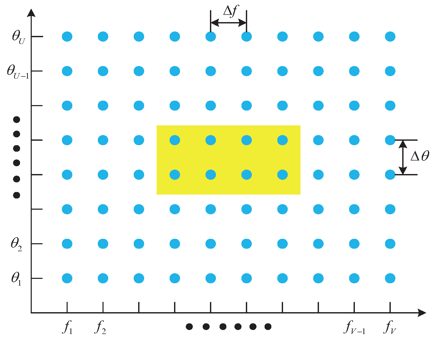
2. ST2D Signal Model of GNSS Receivers

Figure 1 shows a general STAP filter structure for GNSS receiver. Consider a uniform linear array composed of M antenna elements, and the spacing between adjacent elements is d. A temporal filter with N taps and the sampling period $T_s$ is connected behind each antenna element. The received signal of each antenna element is down-converted to the baseband by the radio frequency (RF) front end for the analog-to-digital conversion. After passing through the RF front end, the digitized signal is processed by a FIR filter. Finally, the output signal of the STAP filter is sent to each channel of the GNSS receivers for signal acquisition, tracking, and navigation solution. Consider that the direction of GNSS signal reaching the antenna array is ${\theta }_d$, and the directions of G interferences are ${\theta }_{i_g}(g=1,2,\cdots ,G)$. The received signal vector of the antenna array can be expressed as

$$\begin{array}{cc}\hfill {\mathbf{x}}_1\left(t\right)& ={\mathbf{d}}_1\left(t\right)+{\mathbf{i}}_1\left(t\right)+{\mathbf{n}}_1\left(t\right)\hfill \\ \hfill & ={\mathbf{a}}_s\left({\theta }_d\right)s_d\left(t\right)+\sum _{g=1}^G{\mathbf{a}}_s({\theta }_{i_g})s_{i_g}\left(t\right)+{\mathbf{n}}_1\left(t\right)\hfill \end{array}$$

(1)

where ${\mathbf{d}}_1\left(t\right)$, ${\mathbf{i}}_1\left(t\right)$, and ${\mathbf{n}}_1\left(t\right)$ are respectively the GNSS signal, interference and noise, ${\mathbf{a}}_s\left({\theta }_d\right)$ and ${\mathbf{a}}_s\left({\theta }_{i_g}\right)$ are respectively the steering vectors of the GNSS signal and the g-th interference, $s_d\left(t\right)$ and $s_{i_g}\left(t\right)$ are respectively the complex waveforms of GNSS signal and the g-th interference. The steering vector ${\mathbf{a}}_s\left(\theta \right)\in {\mathbb{C}}^{M\times 1}$ is defined as

$$\begin{array}{c}\hfill {\mathbf{a}}_s\left(\theta \right)={[1,e^{-j2\pi dsin\theta /\lambda },\cdots ,e^{-j2\pi (M-1)dsin\theta /\lambda }]}^T\end{array}$$

(2)

where $\lambda$ is the signal wavelength.

Stack $MN$ time domain snapshots signals into a vector as

$$\begin{array}{cc}\hfill \mathbf{x}\left(t\right)& =\mathbf{d}\left(t\right)+\mathbf{i}\left(t\right)+\mathbf{n}\left(t\right)\hfill \\ \hfill & =({\mathbf{I}}_N\otimes {\mathbf{a}}_s\left({\theta }_d\right)){\mathbf{s}}_d+\sum _{g=1}^G({\mathbf{I}}_N\otimes {\mathbf{a}}_s\left({\theta }_{i_g}\right)){\mathbf{s}}_{i_g}+\mathbf{n}\left(t\right)\hfill \\ \hfill & ={[x_{11}\left(t\right),\cdots ,x_{M1}\left(t\right),\cdots ,x_{1N}\left(t\right),\cdots ,x_{MN}\left(t\right)]}^T\hfill \end{array}$$

(3)

where ${\mathbf{s}}_d={[s_d\left(t\right),\cdots ,s_d(t-(N-1)T_s)]}^T$ and ${\mathbf{s}}_{i_g}={[s_{i_g}\left(t\right),\cdots ,s_{i_g}(t-(N-1)T_s)]}^T$ are the complex envelope sets of the GNSS signal and the g-th interference, respectively. $x_{mn}\left(t\right)$ is the time domain sample at the n-th tap of the temporal filter after the m-th element.

Define the weight vector as $\mathbf{w}={[w_{11},\cdots ,w_{M1},\cdots ,w_{1N},\cdots ,w_{MN}]}^T\in {\mathbb{C}}^{MN\times 1}$, where $w_{mn}$ is the STAP weight at the n-th tap of the temporal filter after the m-th element. The STAP beamformer output can be written as

$$\begin{array}{c}\hfill y={\mathbf{w}}^H\mathbf{x}\left(t\right)=\sum _{m=1}^M\sum _{n=1}^N{w}_{mn}^{*}{x}_{mn}\left(t\right)\end{array}$$

(4)

To generate the weight vector, the well-known Power Inversion (PI) criterion is proposed to minimize the output power of the STAP beamformer. In the PI algorithm, an antenna element is selected as the reference element and the remaining antennas are then viewed as auxiliary elements. The weight vector of the PI algorithm is calculated as

$$\begin{array}{c}\hfill {\mathbf{w}}_{\mathrm{PI}}=\alpha {\mathbf{R}}_{xx}^{-1}\mathbf{c}\end{array}$$

(5)

where $\alpha =1/\left({\mathbf{c}}^H{\mathbf{R}}_{xx}^{-1}\mathbf{c}\right)$ with $\mathbf{c}={[1,0,\cdots ,0]}^T\in {\mathbb{C}}^{MN\times 1}$, and ${\mathbf{R}}_{xx}$ is the auto-correlation matrix of $\mathbf{x}\left(t\right)$ which is denoted as ${\mathbf{R}}_{xx}=E\left\{\mathbf{x}\left(t\right){\mathbf{x}}^H\left(t\right)\right\}$.

3. Proposed Robust STAP Method for GNSS Receivers in Coherent Signal Environments

In this section, a robust STAP MVDR beamforming method for coherent signals in GNSS receivers is proposed. We firstly develop a ST2D-IAA algorithm and modify it to obtain the power spectrum of 2D grid points and the noise power. Then we reconstruct the STINCM for GNSS receivers by using the estimated power spectrum of the interference angle region and the noise power. Furthermore, the STSV of GNSS signal is corrected. Finally, the weight vector of the STAP beamforming is calculated based on the reconstructed STINCM and the corrected STSV of GNSS signal.

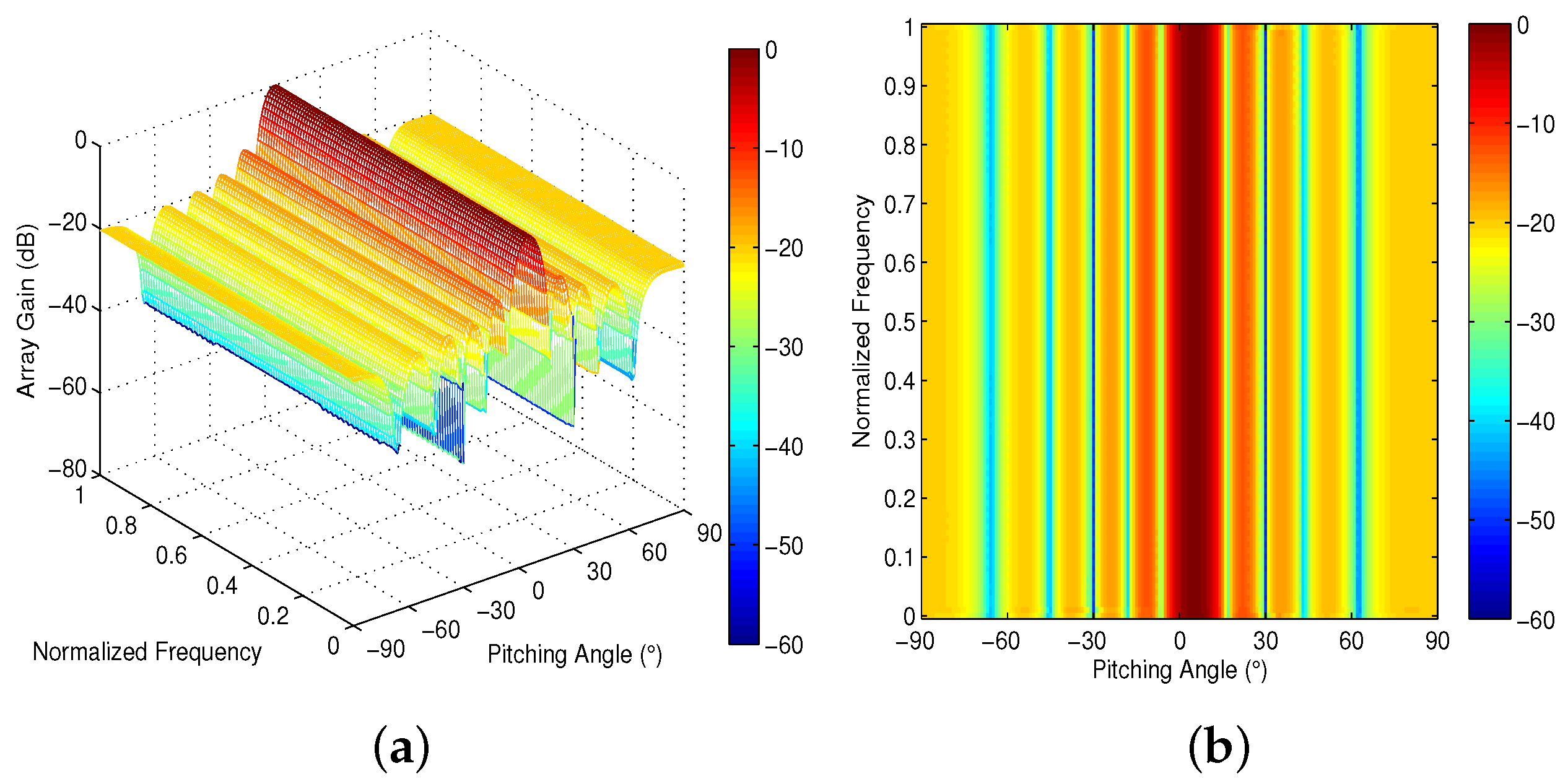
3.1. ST2D-IAA Spectrum Estimation

Considering the STAP beamformer, the ST2D parameters of impinging signals is denoted as

$$\Phi =\left\{(\theta ,f)\right|\theta \in [0,\pi /2],f\in (0,f_h]\}$$

(6)

where $\theta$ represents the pitching angle, f represents the frequency, and $f_h$ represents the cutoff frequency of the low-pass filters in GNSS receivers. The whole space domain $\Theta =\left\{\theta \right|\theta \in [0,\pi /2]\}$ can be uniformly discretized as $\overline{\Theta }=\{{\theta }_1,{\theta }_2,\cdots ,{\theta }_K\}$ by K grid points, and the time domain $\Omega =\left\{f\right|f\in (0,f_h]\}$ can be uniformly discretized as $\overline{\Omega }=\{f_1,f_2,\cdots ,f_L\}$ by L grid points. Accordingly, the joint space-time domain $\Phi$ can be discretized as

$$\overline{\Phi }=\left\{({\theta }_k,f_l)\right|{\theta }_k\in \{{\theta }_1,{\theta }_2,\cdots ,{\theta }_K\},f\in \{f_1,f_2,\cdots ,f_L\}\}$$

(7)

by $K\times L$ 2D grid points. The STSV of the grid point $({\theta }_k,f_l)$ is represented as

$$\mathbf{a}({\theta }_k,f_l)={\mathbf{a}}_s\left({\theta }_k\right)\otimes {\mathbf{a}}_t\left(f_l\right)$$

(8)

for $k=1,2,\cdots ,K$ and $l=1,2,\cdots ,L$. The temporal steering vector ${\mathbf{a}}_t\left(f_l\right)$ is defined as

$${\mathbf{a}}_t\left(f_l\right)={[1,e^{-j2\pi f_l/f_s},\cdots ,e^{-j2\pi (N-1)f_l/f_s}]}^T$$

(9)

where $f_s$ represents the sampling frequency. The space-time steering matrix of all 2D grid points in $\overline{\Phi }$ is denoted as

$$\mathbf{A}=[\mathbf{a}({\theta }_1,f_1),\cdots ,\mathbf{a}({\theta }_1,f_L),\cdots ,\mathbf{a}({\theta }_K,f_1),\cdots ,\mathbf{a}({\theta }_K,f_L)]$$

(10)

The complex envelope vector of all 2D grid points in $\overline{\Phi }$ is written as

$$\mathbf{s}\left(t\right)={[s_{1,1}\left(t\right),\cdots ,s_{1,L}\left(t\right),\cdots ,s_{K,1}\left(t\right),\cdots ,s_{K,L}\left(t\right)]}^T$$

(11)

The power vector of all 2D grid points in $\overline{\Phi }$ is given by

$$\mathbf{p}={[p_{1,1},\cdots ,p_{1,L},\cdots ,p_{K,1},\cdots ,p_{K,L}]}^T$$

(12)

In order to apply the IAA algorithm to the STAP beamforming of GNSS receivers, we propose a ST2D-IAA algorithm to estimate the power spectrum. Similar to the IAA algorithm, we build the weighted least squares cost function for ST2D-IAA algorithm as

$$\begin{array}{c}\hfill \sum _{t=1}^T{\parallel \mathbf{x}\left(t\right)-s_{k,l}\left(t\right)\mathbf{a}({\theta }_k,f_l)\parallel }_{{\mathbf{Q}}^{-1}(k,l)}^2\end{array}$$

(13)

where ${\parallel \mathbf{x}\parallel }_{{\mathbf{Q}}^{-1}(k,l)}^2\triangleq {\mathbf{x}}^H{\mathbf{Q}}^{-1}(k,l)\mathbf{x}$ and the matrix $\mathbf{Q}(k,l)$ is denoted as

$$\begin{array}{c}\hfill \mathbf{Q}(k,l)=\mathbf{R}-p_{k,l}\mathbf{a}({\theta }_k,f_l){\mathbf{a}}^H({\theta }_k,f_l)\end{array}$$

(14)

with

$$\begin{array}{c}\hfill \mathbf{R}=\mathbf{A}\mathrm{diag}\left\{\mathbf{p}\right\}{\mathbf{A}}^H\end{array}$$

(15)

$$\begin{array}{c}\hfill p_{k,l}=\frac{1}{T}\sum _{t=1}^T{\left|s_{k,l}\left(t\right)\right|}^2\end{array}$$

(16)

Minimizing (13) with respect to $s_{k,l}\left(t\right)$ yields

$$\begin{array}{c}\hfill s_{k,l}\left(t\right)=\frac{{\mathbf{a}}^H({\theta }_k,f_l){\mathbf{Q}}^{-1}(k,l)\mathbf{x}\left(t\right)}{{\mathbf{a}}^H({\theta }_k,f_l){\mathbf{Q}}^{-1}(k,l)\mathbf{a}({\theta }_k,f_l)}\end{array}$$

(17)

Using (14) and the matrix inversion lemma (see, e.g., [35]), (17) can be rewritten as

$$\begin{array}{c}\hfill s_{k,l}\left(t\right)=\frac{{\mathbf{a}}^H({\theta }_k,f_l){\mathbf{R}}^{-1}\mathbf{x}\left(t\right)}{{\mathbf{a}}^H({\theta }_k,f_l){\mathbf{R}}^{-1}\mathbf{a}({\theta }_k,f_l)}\end{array}$$

(18)

The steps of the ST2D-IAA algorithm are shown in the Appendix A.1. It should be noted that this algorithm has to be performed in an iterative way because it requires $\mathbf{R}$ which contains the unknown signal powers. The initialization of this algorithm is implemented using a standard delay-and-sum beamformer. Let ${\mathbf{p}}^{\left(i\right)}$ denote the power vector at the i-th iteration in the ST2D-IAA algorithm. The iteration will be terminated when the relative change $\parallel {\mathbf{p}}^{\left(i\right)}-{\mathbf{p}}^{(i-1)}\parallel$ is less than a specified tolerance. Extensive simulations have shown that the number of iterations is less than 12 for the ST2D-IAA algorithm to converge. One can obtain an accurate power spectrum of all 2D grid points from the results of ST2D-IAA algorithm. In addition, the presence of coherent sources has little influence on the performance of ST2D-IAA algorithm.

Although the ST2D-IAA algorithm can obtain accurate power spectrum, it cannot estimate the noise power iteratively. In order to estimate the power spectrum and the noise power simultaneously in the iteration, we further modify the ST2D-IAA algorithm. Based on the weighted least squares method, we modify the optimization problem for estimating $s_{k,l}\left(t\right)$ as below

$$\begin{array}{c}\hfill \underset{s_{k,l}\left(t\right)}{min}\sum _{t=1}^T{\parallel \mathbf{x}\left(t\right)-s_{k,l}\left(t\right)\mathbf{a}({\theta }_k,f_l)\parallel }_{{\overline{\mathbf{R}}}^{-1}}^2\end{array}$$

(19)

where the matrix $\overline{\mathbf{R}}$ is denoted as $\overline{\mathbf{R}}=\mathbf{A}\mathrm{diag}\left\{\overline{\mathbf{p}}\right\}{\mathbf{A}}^H+{\overline{\sigma }}_n^2{\mathbf{I}}_{MN}$ with the power vector $\overline{\mathbf{p}}={[{\overline{p}}_{1,1},\cdots ,{\overline{p}}_{1,L},\cdots ,{\overline{p}}_{K,1},\cdots ,{\overline{p}}_{K,L}]}^T$ and the noise power ${\overline{\sigma }}_n^2$. By iteratively solving (19), $s_{k,l}\left(t\right)$ in the $(i+1)$-th iteration is estimated as

$$\begin{array}{c}\hfill {\overline{s}}_{k,l}^{(i+1)}\left(t\right)=\frac{{\mathbf{a}}^H({\theta }_k,f_l){({\overline{\mathbf{R}}}^{\left(i\right)})}^{-1}\mathbf{x}\left(t\right)}{{\mathbf{a}}^H({\theta }_k,f_l){({\overline{\mathbf{R}}}^{\left(i\right)})}^{-1}\mathbf{a}({\theta }_k,f_l)}\end{array}$$

(20)

where

$$\begin{array}{c}\hfill {\overline{\mathbf{R}}}^{\left(i\right)}=\mathbf{A}\mathrm{diag}\left\{{\overline{\mathbf{p}}}^{\left(i\right)}\right\}{\mathbf{A}}^H+{\left({\overline{\sigma }}_n^2\right)}^{\left(i\right)}{\mathbf{I}}_{MN}\end{array}$$

(21)

$$\begin{array}{c}\hfill {\overline{\mathbf{p}}}^{\left(i\right)}={[{\overline{p}}_{1,1}^{\left(i\right)},\cdots ,{\overline{p}}_{1,L}^{\left(i\right)},\cdots ,{\overline{p}}_{K,1}^{\left(i\right)},\cdots ,{\overline{p}}_{K,L}^{\left(i\right)}]}^T\end{array}$$

(22)

$$\begin{array}{c}\hfill {\overline{p}}_{k,l}^{\left(i\right)}=\frac{1}{T}\sum _{t=1}^T{\left|{\overline{s}}_{k,l}^{\left(i\right)}\left(t\right)\right|}^2\end{array}$$

(23)

$$\begin{array}{c}\hfill {\left({\overline{\sigma }}_n^2\right)}^{\left(i\right)}=\frac{1}{MN}\parallel {(\mathbf{x}\left(t\right)-{\overline{\phi }}^{\left(i\right)}\mathbf{A}{\overline{\mathbf{s}}}^{\left(i\right)}\left(t\right)\parallel }^2\end{array}$$

(24)

$$\begin{array}{c}\hfill {\overline{\mathbf{s}}}^{\left(i\right)}\left(t\right)={[{\overline{s}}_{1,1}^{\left(i\right)}\left(t\right),\cdots ,{\overline{s}}_{1,L}^{\left(i\right)}\left(t\right),\cdots ,{\overline{s}}_{K,1}^{\left(i\right)}\left(t\right),\cdots ,{\overline{s}}_{K,L}^{\left(i\right)}\left(t\right)]}^T\end{array}$$

(25)

where the scaling coefficient ${\overline{\phi }}^{\left(i\right)}$ is obtained from the following optimization problem

$$\begin{array}{c}\hfill \underset{{\overline{\phi }}^{\left(i\right)}}{min}{\parallel \mathbf{x}\left(t\right)-{\overline{\phi }}^{\left(i\right)}\mathbf{A}{\overline{\mathbf{s}}}^{\left(i\right)}\left(t\right)\parallel }^2\end{array}$$

(26)

The solution of (26) is given by

$$\begin{array}{c}\hfill {\overline{\phi }}^{\left(i\right)}=\frac{{\left({\overline{\mathbf{s}}}^{\left(i\right)}\left(t\right)\right)}^H{\mathbf{A}}^H\mathbf{x}\left(t\right)}{{\left({\overline{\mathbf{s}}}^{\left(i\right)}\left(t\right)\right)}^H{\mathbf{A}}^H\mathbf{A}{\overline{\mathbf{s}}}^{\left(i\right)}\left(t\right)}\end{array}$$

(27)

The criterion for the termination of the iteration process (20)–(27) is given by $\parallel {\overline{\mathbf{p}}}^{\left(i\right)}-{\overline{\mathbf{p}}}^{(i-1)}\parallel <\varsigma$. Through extensive simulations, the modified ST2D-IAA algorithm will converge after at most 12 iterations. The steps of the modified ST2D-IAA algorithm are shown in Appendix A.2.

3.2. STINCM Reconstruction

Since the powers of interferences are much higher than those of GNSS signal and noise, the ST2D parameters associated with the interferences can be easily estimated through Pauta criterion. The ST2D parameter of the q-th interference can be denoted as

$$\begin{array}{c}\hfill {\Phi }_g=\left\{(\theta ,f)\right|\theta \in ({\theta }_{i_g},{\theta }_{i_g}+U▵\theta ),f\in (f_{i_g},f_{i_g}+V▵f)\}\end{array}$$

(28)

where $▵\theta$ and $▵f$ denote the spatial and temporal widths occupied by a certain basic 2D subregion, respectively. ${\Phi }_g$ corresponds to the area marked in yellow as shown in Figure 2, which contains the following discretized 2D grid points

$$\begin{array}{cc}\hfill {\overline{\Phi }}_g& =\left\{(\theta ,f)\right|\theta \in \{{\theta }_{i_g,1},\cdots ,{\theta }_{i_g,U}\},f\in \{f_{i_g,1},\cdots ,f_{i_g,V}\}\}\hfill \\ \hfill & =\left\{\begin{array}{cc}\hfill ({\theta }_{i_g,1},& f_{i_g,1})({\theta }_{i_g,1},f_{i_g,2})\cdots ({\theta }_{i_g,1},f_{i_g,V})\hfill \\ \hfill ({\theta }_{i_g,2},& f_{i_g,1})({\theta }_{i_g,2},f_{i_g,2})\cdots ({\theta }_{i_g,2},f_{i_g,V})\hfill \\ \hfill & ⋮⋮\ddots ⋮\hfill \\ \hfill ({\theta }_{i_g,U},& f_{i_g,1})({\theta }_{i_g,U},f_{i_g,2})\cdots ({\theta }_{i_g,U},f_{i_g,V})\hfill \end{array}\right\}\hfill \end{array}$$

(29)

The ST2D steering matrix corresponding to ${\overline{\Phi }}_g$ can be denoted as

$$\begin{array}{c}\hfill \mathbf{A}\left({\overline{\Phi }}_g\right)=[\mathbf{a}({\theta }_{i_g,1},f_{i_g,1}),\cdots ,\mathbf{a}({\theta }_{i_g,1},f_{i_g,V}),\cdots ,\mathbf{a}({\theta }_{i_g,U},f_{i_g,1}),\cdots ,\mathbf{a}({\theta }_{i_g,U},f_{i_g,V})]\end{array}$$

(30)

Based on the results of modified ST2D-IAA algorithm, the ST2D spectrum estimation vector corresponding to ${\overline{\Phi }}_g$ can be written as

$$\begin{array}{cc}\hfill \overline{\mathbf{p}}\left({\overline{\Phi }}_g\right)=[& \overline{p}({\theta }_{i_g,1},f_{i_g,1}),\cdots ,\overline{p}({\theta }_{i_g,1},f_{i_g,V}),\cdots ,\overline{p}({\theta }_{i_g,U},f_{i_g,1}),\cdots ,\overline{p}({\theta }_{i_g,U},f_{i_g,V}){]}^T\hfill \end{array}$$

(31)

Considering all of the ST2D steering matrices $\mathbf{A}\left({\overline{\Phi }}_g\right),g=1,\cdots ,G$ and the ST2D spectrum estimation vectors $\overline{\mathbf{p}}\left({\overline{\Phi }}_g\right),g=1,\cdots ,G$, we can construct the space-time interference covariance matrix as

$$\begin{array}{cc}\hfill {\widehat{\mathbf{R}}}_i& =\sum _{g=1}^G\mathbf{A}\left({\overline{\Phi }}_g\right)\mathrm{diag}\left\{\overline{\mathbf{p}}\left({\overline{\Phi }}_g\right)\right\}{\mathbf{A}}^H\left({\overline{\Phi }}_g\right)\hfill \\ \hfill & =\sum _{g=1}^G\sum _{u=1}^U\sum _{v=1}^V\overline{p}({\theta }_{i_g,u},f_{i_g,v})\mathbf{a}({\theta }_{i_g,u},f_{i_g,v}){\mathbf{a}}^H({\theta }_{i_g,u},f_{i_g,v})\hfill \end{array}$$

(32)

The final noise power ${\overline{\sigma }}_n^2$ can be obtained from the modified ST2D-IAA algorithm. Thus, the noise covariance matrix can be estimated as

$$\begin{array}{c}\hfill {\widehat{\mathbf{R}}}_n={\overline{\sigma }}_n^2{\mathbf{I}}_{MN}\end{array}$$

(33)

By using the constructed space-time interference covariance matrix ${\widehat{\mathbf{R}}}_i$ and the noise covariance matrix ${\widehat{\mathbf{R}}}_n$, we reconstruct the STINCM as

$$\begin{array}{cc}\hfill {\widehat{\mathbf{R}}}_{in}=& {\widehat{\mathbf{R}}}_i+{\widehat{\mathbf{R}}}_n\hfill \\ \hfill =& \sum _{g=1}^G\sum _{u=1}^U\sum _{v=1}^V\overline{p}({\theta }_{i_g,u},f_{i_g,v})\mathbf{a}({\theta }_{i_g,u},f_{i_g,v}){\mathbf{a}}^H({\theta }_{i_g,u},f_{i_g,v})+{\overline{\sigma }}_n^2{\mathbf{I}}_{MN}\hfill \end{array}$$

(34)

3.3. STSV Estimation

In order to suppress the interferences with high powers while remaining a distortionless response for the GNSS signal, we formulate the optimization problem of the STAP beamforming based on the MVDR criterion as

$$\begin{array}{cc}\hfill \underset{\mathbf{w}}{min}& {\mathbf{w}}^H{\mathbf{R}}_{in}\mathbf{w}\hfill \\ \hfill \mathrm{subject}\mathrm{to}& N\mathrm{is}\mathrm{odd}\hfill \\ \hfill & {\mathbf{w}}^H\mathbf{a}=1\hfill \\ \hfill & \mathbf{a}={[\underset{M(N-1)/2}{\underbrace{0,\cdots ,0}},{\mathbf{a}}_s\left({\theta }_d\right),\underset{M(N-1)/2}{\underbrace{0,\cdots ,0}}]}^T\hfill \end{array}$$

(35)

where ${\mathbf{R}}_{in}=E\left\{(\mathbf{i}\left(t\right)+\mathbf{n}\left(t\right)){(\mathbf{i}\left(t\right)+\mathbf{n}\left(t\right))}^H\right\}\in {\mathbb{C}}^{MN\times MN}$ represents the theoretical STINCM. The constraints in (35) are imposed to guarantee the linearity of the STAP beamforming response so that no biases are introduced into the code and carrier phase measurements [12]. The optimal solution of (35) is given by

$${\mathbf{w}}_{opt}=\frac{{\mathbf{R}}_{in}^{-1}\mathbf{a}}{{\mathbf{a}}^H{\mathbf{R}}_{in}^{-1}\mathbf{a}}$$

(36)

Since ${\mathbf{R}}_{in}$ is unavailable in practice, we replace it with the reconstructed STINCM ${\widehat{\mathbf{R}}}_{in}$ in (34). Besides, the STSV $\mathbf{a}$ is not accurate because it may have STSV error caused by many factors in practical circumstances. By taking the STSV error $\mathbf{e}$ into account, the actual STSV can be written as $\mathbf{a}+\mathbf{e}$. Based on the reconstructed STINCM ${\widehat{\mathbf{R}}}_{in}$ and the actual STSV $\mathbf{a}+\mathbf{e}$, the STAP beamformer output power can be denoted as

$$\widehat{P}(\mathbf{a}+\mathbf{e})=\frac{1}{{(\mathbf{a}+\mathbf{e})}^H{\widehat{\mathbf{R}}}_{in}^{-1}(\mathbf{a}+\mathbf{e})}$$

(37)

The STSV error $\mathbf{e}$ can be estimated by maximizing $\widehat{P}(\mathbf{a}+\mathbf{e})$ or, equivalently, by minimizing the denominator of $\widehat{P}(\mathbf{a}+\mathbf{e})$. The STSV error $\mathbf{e}$ can be further decomposed into the orthogonal component ${\mathbf{e}}_{\perp }$ and the parallel component ${\mathbf{e}}_{\Vert }$. Since the parallel component ${\mathbf{e}}_{\Vert }$ does not have influence on the STAP beamforming performance, we dismiss ${\mathbf{e}}_{\Vert }$ and only take ${\mathbf{e}}_{\perp }$ into computation. The optimization problem for estimating ${\mathbf{e}}_{\perp }$ can be formulated as

$$\begin{array}{cc}\hfill \underset{{\mathbf{e}}_{\perp }}{min}& {(\mathbf{a}+{\mathbf{e}}_{\perp })}^H{\widehat{\mathbf{R}}}_{in}^{-1}(\mathbf{a}+{\mathbf{e}}_{\perp })\hfill \\ \hfill \mathrm{subject}\mathrm{to}& {\mathbf{a}}^H{\mathbf{e}}_{\perp }=0\hfill \\ \hfill & {(\mathbf{a}+{\mathbf{e}}_{\perp })}^H{\widehat{\mathbf{R}}}_{in}(\mathbf{a}+{\mathbf{e}}_{\perp })\le {\mathbf{a}}^H{\widehat{\mathbf{R}}}_{in}\mathbf{a}\hfill \end{array}$$

(38)

Since ${\widehat{\mathbf{R}}}_{in}^{-1}\succ 0$ with the symbol ≻ denoting the positive-definite operation, the convex optimization problem (38) can be easily solved to obtain the solution ${\widehat{\mathbf{e}}}_{\perp }$. With the estimated ${\widehat{\mathbf{e}}}_{\perp }$, the STSV $\mathbf{a}$ can be corrected as

$$\begin{array}{c}\hfill \widehat{\mathbf{a}}=\mathbf{a}+{\widehat{\mathbf{e}}}_{\perp }\end{array}$$

(39)

From the last constraint in the optimization problem (35), it can be seen that the corrected STSV $\widehat{\mathbf{a}}$ should satisfy $\widehat{\mathbf{a}}={[{\displaystyle \underset{M(N-1)/2}{{\displaystyle \underbrace{0,\cdots ,0}}}},{\widehat{\mathbf{a}}}_s\left({\theta }_d\right),\underset{M(N-1)/2}{{\displaystyle \underbrace{0\cdots ,0}}}]}^T$. It means that ${\widehat{\mathbf{a}}}_s\left({\theta }_d\right)$ can be denoted as ${\widehat{\mathbf{a}}}_s\left({\theta }_d\right)=\widehat{\mathbf{a}}(\frac{MN-M+2}{2}:\frac{M(N+1)}{2})$. The optimal weight vector is obtained as

$$\begin{array}{c}\hfill \widehat{\mathbf{w}}=\frac{{\widehat{\mathbf{R}}}_{in}^{-1}\widehat{\mathbf{a}}}{{\widehat{\mathbf{a}}}^H{\widehat{\mathbf{R}}}_{in}^{-1}\widehat{\mathbf{a}}}\end{array}$$

(40)

It should be mentioned that the GNSS signal is generated with the direct-sequence spread-spectrum (DSSS) technique, which shows that it lies in the whole frequency band after passing through low-pass filters in GNSS receivers. In other words, the STSV of the GNSS signal does not have the form $\mathbf{a}({\theta }_d,f_d)={\mathbf{a}}_s\left({\theta }_d\right)\otimes {\mathbf{a}}_t\left(f_d\right)$ with a certain frequency $f_d$. Therefore, the constraints of the optimization problem (35) have to be revised for the GNSS signal. The revised optimization problem can be obtained from

$$\begin{array}{cc}\hfill \underset{\mathbf{w}}{min}& {\mathbf{w}}^H{\widehat{\mathbf{R}}}_{in}\mathbf{w}\hfill \\ \hfill \mathrm{subject}\mathrm{to}& N\mathrm{is}\mathrm{odd}\hfill \\ \hfill & {\mathbf{w}}^H\mathbf{C}=\mathbf{f}\hfill \\ \hfill & \mathbf{C}={\left[\begin{array}{cccc}{\widehat{\mathbf{a}}}_s\left({\theta }_d\right)& \mathbf{0}& \cdots & \mathbf{0}\\ \mathbf{0}& {\widehat{\mathbf{a}}}_s\left({\theta }_d\right)& \cdots & \mathbf{0}\\ ⋮& ⋮& \ddots & ⋮\\ \mathbf{0}& \mathbf{0}& \cdots & {\widehat{\mathbf{a}}}_s\left({\theta }_d\right)\end{array}\right]}_{MN\times N}\hfill \\ \hfill & \mathbf{f}={[\underset{(N-1)/2}{\underbrace{0,\cdots ,0}},1,\underset{(N-1)/2}{\underbrace{0,\cdots ,0}}]}^T\hfill \end{array}$$

(41)

By solving (41), the final weight vector can be given by

$$\begin{array}{c}\hfill \overline{\mathbf{w}}={\widehat{\mathbf{R}}}_{in}^{-1}\mathbf{C}{\left[{\mathbf{C}}^H{\widehat{\mathbf{R}}}_{in}^{-1}\mathbf{C}\right]}^{-1}\mathbf{f}\end{array}$$

(42)

Based on the weight vector in (42), the array output carrier-to-noise ratio $C/N_0$ of the GNSS signal can be denoted as

$$C/N_0=\frac{B{\sigma }_d^2{\left|{\mathbf{w}}^H\mathbf{C}\right|}^2}{{\mathbf{w}}^H{\widehat{\mathbf{R}}}_{in}\mathbf{w}}$$

(43)

where B denotes the signal bandwidth and ${\sigma }_d^2$ denotes the power of the GNSS signal.

The work [36] assesses the performance of receivers by measuring a zero baseline and a short baseline in the field. In the short baseline test, the multipath error is compensated by a set of harmonic functions, which can guarantee the property of unbiasedness of the least-squares estimators. However, The least-squares method provided in [36] may be less agile than the proposed method of this paper in terms of iterations.

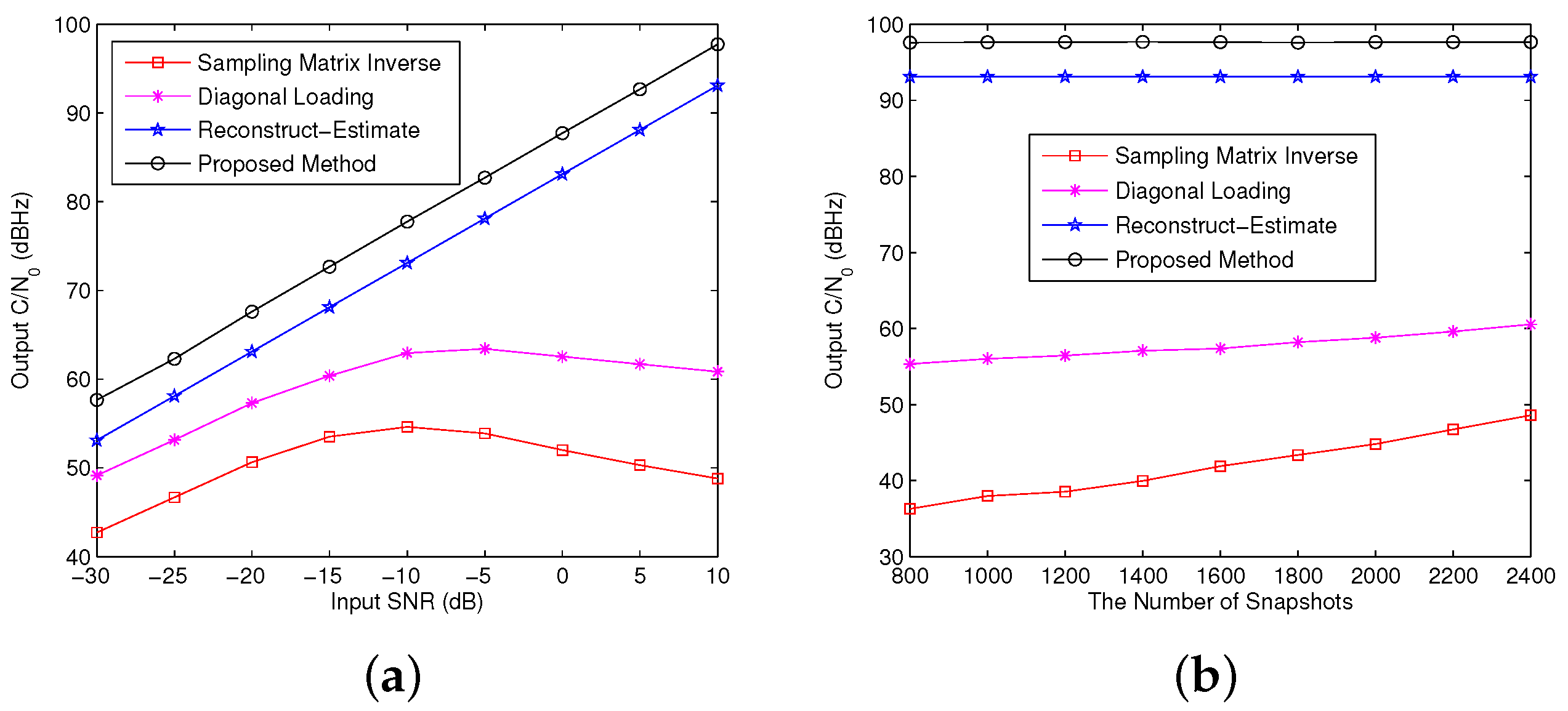
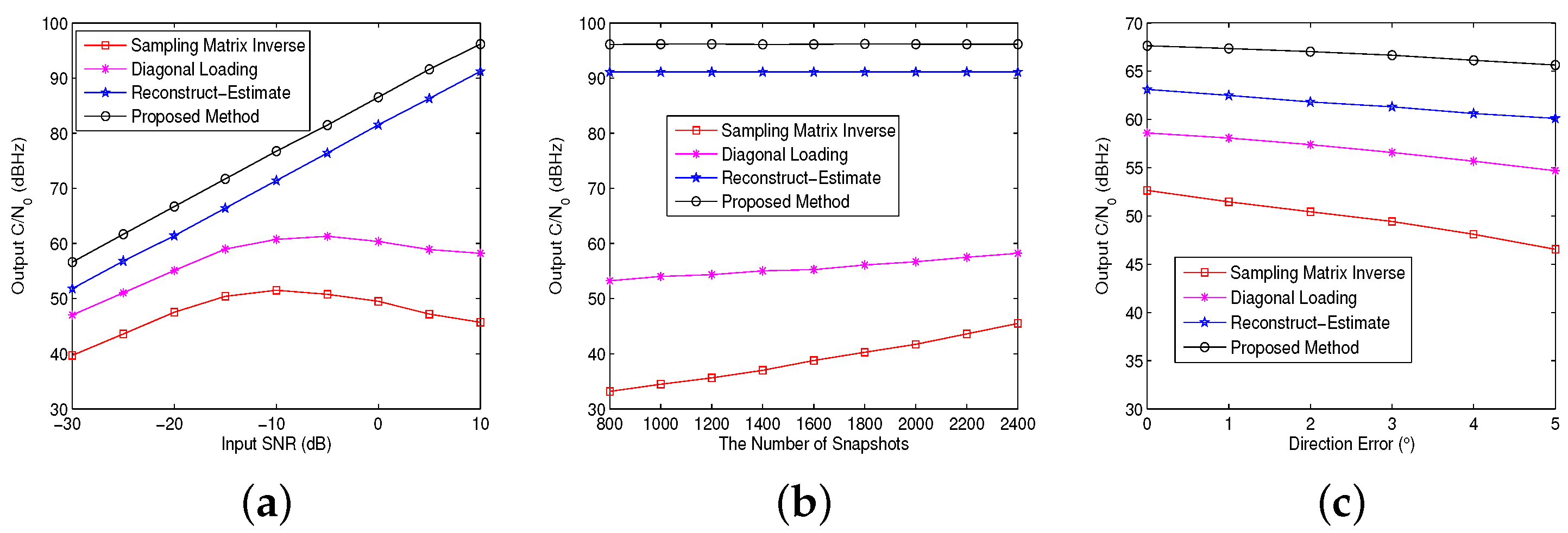
4. Simulation Results

Consider a uniform linear array consisting of 10 omnidirectional elements with half wavelength spacing and each element is followed by 8-order FIR filter. The desired GNSS signal is assumed as BeiDou-2 (BD2) signal at B3 band whose carrier frequency is 1268.52 MHz and mainlobe bandwidth is 20.46 MHz. The desired BD2 signal impinges on the array from the direction ${\theta }_d=5^{\circ }$. Two interferences whose bandwidths are the same as the desired BD2 signal are respectively incident from the directions ${\theta }_{i_1}={30}^{\circ }$ and ${\theta }_{i_2}=-{30}^{\circ }$ and the common INR is 30 dB. Only the interference from the direction ${30}^{\circ }$ is coherent with the desired BD2 signal. In coherent signal environment, the number of samples utilized to calculate the weight vector is chosen as 2400.

Firstly, the spatial-temporal beampatterns corresponding to the proposed method are obtained to observe whether nulls are formed in the directions of interferences. Then, the output $C/N_0$ performance of the proposed method is mainly compared with the sample matrix inverse method in [37], the diagonal loading in [10], the reconstruct-estimate method in [38]. Although the sampling matrix inverse method is widely used to calculate the weighted vector of STAP beamformers, it can neither suppress the interferences in the coherent signal environments nor be robust to the STSV error caused by the model errors. As for the diagonal loading method, it is a widely used method to deal with space-time covariance matrix errors. The reconstruct-estimate method is also an INCM reconstruction method with STAP structure, which is robust to model errors. In order to verify the robustness of the proposed method in the coherent signal environments and model error conditions, the above methods are selected for comparison. In the reconstruct-estimate method, the angle region of the desired BD2 signal is $[{\theta }_d-5^{\circ },{\theta }_d+5^{\circ }]$. In the proposed method of this paper, the two interference angle regions are $[{\theta }_{i_1}-{10}^{\circ },{\theta }_{i_1}+{10}^{\circ }]$ and $[{\theta }_{i_2}-{10}^{\circ },{\theta }_{i_2}+{10}^{\circ }]$, respectively. The threshold $\varsigma$ is set to ${10}^{-3}$.

Example 1: Spatial-temporal beampatterns. The 3D and 2D spatial-temporal beampatterns of the proposed method are shown in Figure 3a and Figure 3b respectively. It can be seen that while the entire frequency band at the desired BD2 signal direction forms a mainlobe, nullings are formed in the entire frequency bands of the interference directions ${30}^{\circ }$ and $-{30}^{\circ }$, respectively. This shows that the proposed STAP beamforming method can effectively suppress the interferences in the coherent signal environments, because the proposed method uses the modified ST2D-IAA method to estimate the precise power spectrum.

Example 2: Output $C/N_0$ performance.Figure 4a shows the relationship curves of the sampling matrix inverse method, diagonal loading method, reconstruct-estimate method and the proposed method with the change of the output $C/N_0$ versus the input SNR. Note that although the GNSS signal input SNR is usually $-20$ dB, the spot beam has been or will be equipped with modern GNSS in the future, so the corresponding SNR will be increased to 27 dB, so the SNR range of BD2 signal is $[-30,10]$ dB. It can be seen from Figure 4a that the output $C/N_0$ performance of the proposed method is better than those of the other methods, because the proposed method can suppress the interferences in the coherent signal environments, while the other methods cannot deal with the interferences in the coherent signal environments. Figure 4b shows the relationship curves of the sampling matrix inverse method, diagonal loading method, reconstruct-estimate method and the proposed method with the change of the output $C/N_0$ versus the number of snapshots. It can be seen that the output $C/N_0$ performance of the proposed method is still better than the other methods, and the proposed method has good advantages in the output $C/N_0$.

Example 3: The scenary of direction error. When the direction error of the desired BD2 signal is $3^{\circ }$, that is, the actual direction of the BD2 signal is $8^{\circ }$. In this case, Figure 5a and Figure 5b respectively show the relationship curves of the change of the output $C/N_0$ versus the input SNR and the number of snapshots, while Figure 5c shows the relationship curves of the output $C/N_0$ versus the direction error. It can be seen from these figures that both the proposed method and the reconstruct-estimate method are robust to the signal direction error, because both of them consider the signal STSV error and correct the signal STSV. However, the performance of the diagonal loading method and the sampling matrix inverse method is poor in the case of signal direction error, because these two methods do not consider the signal STSV error, and do not correct the signal STSV. In addition, the proposed method has the best performance of the output $C/N_0$, which is because the proposed method not only reconstructs the STINCM, but also corrects the signal STSV.

Example 4: The case of arbitrary STSV error. In the case of arbitrary STSV error of the signal, the actual STSV of the desired BD2 signal can be expressed as $\mathbf{a}=\mathbf{a}({\theta }_d+\delta \theta )+\delta \mathbf{a}$, where the direction error $\delta \theta$ is fixed at $3^{\circ }$, the STSV error $\delta \mathbf{a}$ is a random vector with the mean 0 and the variance ${\sigma }^2{\mathbf{I}}_{MN\times 1}$. The parameter ${\sigma }^2$ is set to $0.64$. Figure 6a and Figure 6b respectively show the relationship curves of output $C/N_0$ versus the input SNR and versus the number of snapshots under the condition of arbitrary STSV error of the signal. It can be seen that the output $C/N_0$ of the proposed method is higher than that of the other methods, because the proposed method combines the accurate STINCM and the corrected STSV, which indicates that the proposed method is robust to arbitrary STSV error of signal.

Example 5: The situation of small number of snapshots. We investigate the performance of the tested methods when the number of snapshots is small. The simulated curves of output $C/N_0$ versus the number of snapshots are displayed in Figure 7, where the number of snapshots ranges from 20 to 200. Obviously, the proposed method has the minimal performance loss, and performs better than the other methods in the situation of small number of snapshots. The reason lies in that the ST2D-IAA spectrum estimation in the proposed method can work with the limited sampling snapshots. As described in [33], the IAA spectrum estimation can even handle the single snapshot in the coprime virtual uniform linear array. Therefore, the performance of the proposed method is robust against the small number of snapshots.

5. Conclusions

In this paper, a robust STAP method based on the modified ST2D-IAA spectrum estimation is proposed to suppress interferences for GNSS receivers in coherent signal environments. By applying the IAA algorithm to the ST2D signal model in GNSS receivers and further modifying the ST2D-IAA algorithm, the power spectrum and noise power can be estimated accurately at the same time. The STINCM of GNSS receivers is reconstructed by selecting the estimated power spectrum and noise power corresponding to the interference angle regions. In order to obtain the error vector of the STSV, the STAP beamforming optimization problem based on the MVDR criterion is constructed to correct the STSV of GNSS signal. The weight vector of STAP beamforming is calculated by combining the reconstructed STINCM and the corrected GNSS signal STSV. Simulation results show that the proposed method can suppress the interferences in the coherent signal environments, and has better robustness than the existing methods under the conditions of model errors. The proposed method has a potential prospect in maintaining the integrity and functionality of GNSS systems against coherent interference in many applications.

References

1. Marut, G.; Hadas, T.; Kaplon, J.; Trzcina, E.; Rohm, W. Monitoring the water vapor content at high spatio-temporal resolution using a network of low-cost multi-GNSS receivers. IEEE Trans. Geosci. Remote Sens. 2022, 60, 5804614. [Google Scholar] [CrossRef]
2. Suzuki, T. GNSS Odometry: Precise trajectory estimation based on carrier phase cycle slip estimation. IEEE Robot. Autom. Lett. 2022, 7, 7319–7326. [Google Scholar] [CrossRef]
3. Osechas, O.; Fohlmeister, F.; Dautermann, T.; Felux, M. Impact of GNSS-band radio interference on operational avionics. Navig. J. Inst. Navig. 2022, 69, navi.516. [Google Scholar] [CrossRef]
4. Chen, X.; He, D.; Yan, X.; Yu, W.; Truong, T.K. GNSS interference type recognition with fingerprint spectrum DNN method. IEEE Trans. Aerosp. Electron. Syst. 2022, 58, 4745–4760. [Google Scholar] [CrossRef]
5. Meng, L.; Yang, L.; Yang, W.; Zhang, L. A survey of GNSS spoofing and anti-spoofing technology. Remote Sens. 2022, 14, 4826. [Google Scholar] [CrossRef]
6. Huang, L.; Lu, Z.; Xiao, Z.; Ren, C.; Song, J.; Li, B. Suppression of jammer multipath in GNSS antenna array receiver. Remote Sens. 2022, 14, 350. [Google Scholar] [CrossRef]
7. Lu, Z.; Song, J.; Huang, L.; Ren, C.; Xiao, Z.; Li, B. Distortionless 1/2 overlap windowing in frequency domain anti-jamming of satellite navigation receivers. Remote Sens. 2022, 14, 1801. [Google Scholar] [CrossRef]
8. Zhang, J.; Feng, W.; Yuan, T.; Wang, J.; Sangaiah, A.K. SCSTCF: Spatial-channel selection and temporal regularized correlation filters for visual tracking. Appl. Soft Comput. 2022, 118, 108485. [Google Scholar] [CrossRef]
9. Zhou, M.; Wang, Q.; He, F.; Meng, J. Impacts of phase noise on the anti-jamming performance of power inversion algorithm. Sensors 2022, 22, 2362. [Google Scholar] [CrossRef]
10. Cox, H.; Zeskind, R.M.; Owen, M.M. Robust adaptive beamforming. IEEE Trans. Acoust. Speech Signal Process. 1987, 35, 1365–1376. [Google Scholar] [CrossRef]
11. Zhang, W.; Liu, T.; Yang, G.; Jiang, C.; Hu, Y.; Lan, T.; Zhao, Z. A novel method for improving quality of oblique incidence sounding ionograms based on eigenspace-based beamforming technology and Capon high-resolution range profile. Remote Sens. 2022, 14, 4305. [Google Scholar] [CrossRef]
12. Huang, Y.; Fu, H.; Vorobyov, S.A.; Luo, Z.Q. Robust adaptive beamforming via worst-case sinr maximization with nonconvex uncertainty sets. IEEE Trans. Signal Process. 2023, 71, 218–232. [Google Scholar] [CrossRef]
13. Gu, Y.; Leshem, A. Robust adaptive beamforming based on interference covariance matrix reconstruction and steering vector estimation. IEEE Trans. Signal Process. 2012, 60, 3881–3884. [Google Scholar]
14. Meng, Z.; Dong, S.; Shi, X.; Wang, X. Robust beamforming for non-circular signals in uniform linear arrays with unknown mutual couplin. Digit. Signal Process. 2022, 122, 103378. [Google Scholar] [CrossRef]
15. Li, H.; Geng, J.; Xie, J. Robust adaptive beamforming based on covariance matrix reconstruction with RCB principle. Digit. Signal Process. 2022, 127, 103565. [Google Scholar] [CrossRef]
16. Meng, Z.; Zhou, W. Robust adaptive beamforming for coprime array with steering vector estimation and covariance matrix reconstruction. IET Commun. 2020, 14, 2749–2758. [Google Scholar] [CrossRef]
17. Xie, Y.; Chen, F.; Huang, L.; Liu, Z.; Wang, F. Carrier phase bias correction for GNSS space-time array processing using time-delay data. GPS Solut. 2023, 27, 113. [Google Scholar] [CrossRef]
18. Hao, F.; Li, X.; Wang, W.; Zhao, J. A STAP anti-interference technology with zero phase bias in wireless IoT systems based on high-precision positioning. Front. Phys. 2023, 11, 284. [Google Scholar] [CrossRef]
19. Stenberg, N.; Axell, E.; Rantakokko, J.; Hendeby, G. Results on GNSS spoofing mitigation using multiple receivers. Navig. J. Inst. Navig. 2022, 69, navi.510. [Google Scholar] [CrossRef]
20. Wang, Y.; Liu, W.; Huang, L.; Xiao, Z.; Wang, F. Distortionless pseudo-code tracking space-time adaptive processor based on the PI criterion for GNSS receiver. IET Radar Sonar Navig. 2020, 14, 1984–1990. [Google Scholar] [CrossRef]
21. Brachvogel, M.; Niestroj, M.; Meurer, M.; Hasnain, S.N.; Stephan, R.; Hein, M.A. Space-time adaptive processing as a solution for mitigating interference using spatially-distributed antenna arrays. Navig. J. Inst. Navig. 2023, 70, navi.592. [Google Scholar] [CrossRef]
22. Chen, X.; Morton, Y. Iterative subspace alternating projection method for GNSS multipath DOA estimation. IET Radar Sonar Navig. 2016, 10, 1260–1269. [Google Scholar] [CrossRef]
23. Ghiasi, Y.; Duguay, C.R.; Murfitt, J.; van der Sanden, J.J.; Thompson, A.; Drouin, H.; Prévost, C. Application of GNSS interferometric reflectometry for the estimation of lake ice thickness. Remote Sens. 2020, 12, 2721. [Google Scholar] [CrossRef]
24. Wen, F.; Shi, J.; Zhang, Z. Generalized spatial smoothing in bistatic EMVS-MIMO radar. Signal Process. 2022, 193, 108406. [Google Scholar] [CrossRef]
25. Shi, J.; Yang, Z.; Liu, Y. On parameter identifiability of diversity-smoothing-based MIMO radar. IEEE Trans. Aerosp. Electron. Syst. 2021, 58, 1660–1675. [Google Scholar] [CrossRef]
26. Pote, R.R.; Rao, B.D. Maximum likelihood-based gridless doa estimation using structured covariance matrix recovery and sbl with grid refinement. IEEE Trans. Signal Process. 2023, 71, 802–815. [Google Scholar] [CrossRef]
27. Rahamim, D.; Tabrikian, J.; Shavit, R. Source localization using vector sensor array in a multipath environment. IEEE Trans. Signal Process. 2004, 52, 3096–3103. [Google Scholar] [CrossRef]
28. He, J.; Jiang, S.; Wang, J.; Liu, Z. Polarization difference smoothing for direction finding of coherent signals. IEEE Trans. Aerosp. Electron. Syst. 2010, 46, 469–480. [Google Scholar] [CrossRef]
29. Zhang, Z.; Wen, F.; Shi, J.; He, J.; Truong, T.K. 2D-DOA estimation for coherent signals via a polarized uniform rectangular array. IEEE Signal Process. Lett. 2023, 30, 893–897. [Google Scholar] [CrossRef]
30. Park, Y.; Gerstoft, P. Gridless sparse covariance-based beamforming via alternating projections including co-prime arrays. J. Acoust. Soc. Am. 2022, 151, 3828–3837. [Google Scholar] [CrossRef] [PubMed]
31. Mao, D.; Zhang, Y.; Zhang, Y.; Huo, W.; Pei, J.; Huang, Y. Target fast reconstruction of real aperture radar using data extrapolation-based parallel iterative adaptive approach. IEEE J. Sel. Top. Appl. Earth Obs. Remote Sens. 2021, 14, 2258–2269. [Google Scholar] [CrossRef]
32. Wang, B.; Li, S.; Battistelli, G.; Chisci, L. Fast iterative adaptive approach for indoor localization with distributed 5G small cells. IEEE Wirel. Commun. Lett. 2022, 11, 1980–1984. [Google Scholar] [CrossRef]
33. Meng, Z.; Zhou, W. Virtual uniform linear iterative adaptive approach for robust adaptive beamforming. In Proceedings of the 2020 39th Chinese Control Conference (CCC), Shenyang, China, 27–29 July 2020; pp. 2980–2985. [Google Scholar]
34. Yang, X.; Xie, J.; Li, H.; He, Z. Robust adaptive beamforming of coherent signals in the presence of the unknown mutual coupling. IET Commun. 2018, 12, 75–81. [Google Scholar] [CrossRef]
35. Stoica, P.; Moses, R.L. Spectral Analysis of Signals; Prentice Hall: Upper Saddle River, NJ, USA, 2005. [Google Scholar]
36. Amiri-Simkooei, A.R.; Tiberius, C.C.J.M. Assessing receiver noise using GPS short baseline time series. GPS Solut. 2007, 11, 21–35. [Google Scholar] [CrossRef]
37. Capon, J. High-resolution frequency-wavenumber spectrum analysis. Proc. IEEE 1969, 57, 1408–1418. [Google Scholar] [CrossRef]
38. Li, Z.; Zhang, Y.; Liu, H. A robust STAP method for airborne radar based on clutter covariance matrix reconstruction and steering vector estimation. Digit. Signal Process. 2018, 78, 82–91. [Google Scholar] [CrossRef]
Figure 1. General STAP filter structure for GNSS receiver.
Remotesensing 15 04212 g001
Figure 2. Division of the joint space-time domain for the STAP architecture.
Remotesensing 15 04212 g002
Figure 3. The spatial-temporal beampatterns of the proposed method. (a) 3D spatial-temporal beampattern. (b) 2D spatial-temporal beampattern.
Remotesensing 15 04212 g003
Figure 4. The simulation results in example 2. (a) output C / N 0 versus the input SNR. (b) output C / N 0 versus the number of snapshots.
Remotesensing 15 04212 g004
Figure 5. The simulation results in example 3. (a) output C / N 0 versus the input SNR. (b) output C / N 0 versus the number of snapshots. (c) output C / N 0 versus the direction error.
Remotesensing 15 04212 g005
Figure 6. The simulation results in example 4. (a) output C / N 0 versus the input SNR. (b) output C / N 0 versus the number of snapshots.
Remotesensing 15 04212 g006
Figure 7. The simulation results in example 5. Output C / N 0 versus the number of snapshots.
Remotesensing 15 04212 g007
Disclaimer/Publisher’s Note: The statements, opinions and data contained in all publications are solely those of the individual author(s) and contributor(s) and not of MDPI and/or the editor(s). MDPI and/or the editor(s) disclaim responsibility for any injury to people or property resulting from any ideas, methods, instructions or products referred to in the content.