UCTNet with Dual-Flow Architecture: Snow Coverage Mapping with Sentinel-2 Satellite Imagery

Abstract

Satellite remote sensing (RS) has been drawing considerable research interest in land-cover classification due to its low price, short revisit time, and large coverage. However, clouds pose a significant challenge, occluding the objects on satellite RS images. In addition, snow coverage mapping plays a vital role in studying hydrology and climatology and investigating crop disease overwintering for smart agriculture. Distinguishing snow from clouds is challenging since they share similar color and reflection characteristics. Conventional approaches with manual thresholding and machine learning algorithms (e.g., SVM and Random Forest) could not fully extract useful information, while current deep-learning methods, e.g., CNNs or Transformer models, still have limitations in fully exploiting abundant spatial/spectral information of RS images. Therefore, this work aims to develop an efficient snow and cloud classification algorithm using satellite multispectral RS images. In particular, we propose an innovative algorithm entitled UCTNet by adopting a dual-flow structure to integrate information extracted via Transformer and CNN branches. Particularly, CNN and Transformer integration Module (CTIM) is designed to maximally integrate the information extracted via two branches. Meanwhile, Final Information Fusion Module and Auxiliary Information Fusion Head are designed for better performance. The four-band satellite multispectral RS dataset for snow coverage mapping is adopted for performance evaluation. Compared with previous methods (e.g., U-Net, Swin, and CSDNet), the experimental results show that the proposed UCTNet achieves the best performance in terms of accuracy (95.72%) and mean IoU score (91.21%) while with the smallest model size (3.93 M). The confirmed efficiency of UCTNet shows great potential for dual-flow architecture on snow and cloud classification.

1. Introduction

Land-cover classification via satellite remote sensing (RS) images is an essential task in the field of earth observation. It has been widely applied in various areas, such as land water resources, vegetation resources, environmental monitoring, natural disaster forecasting [1], urban planning [2,3,4,5], environmental impact assessment [6,7], and precision agriculture [8,9]. In particular, Sentinel-2 series satellites, one of the main RS platforms for land cover mapping, are capable of enabling persistent sensing for civil applications because of their multispectral information via customized sensors with high spatial/spectral/temporal resolutions in a wide range. However, as reported in [10], 66% of Earth’s surface is covered by clouds. As a result, clouds inevitably appear on the acquired satellite images, restricting their applications in land-cover classification [11]. Meanwhile, it is also reported in [12] that snow coverage mapping plays an important role not only in studying hydrology and climatology but also in investigating crop disease overwintering for smart agriculture since snow coverage in winter not only weakens the negative effects of extreme cold temperature on crops but also have certain protection effects on crop diseases (e.g., yellow rust disease in wheat [13]). Considering that snow and clouds share a very similar appearance and color distribution, manually separating snow pixels from cloud pixels requires expert knowledge and is a tedious and time-consuming process. Therefore, it is desirable to develop an automated algorithm to discriminate cloud/snow in RS images, facilitating the post-processing operations and interpretation of RS images, which is highly beneficial for land cover classification and precision agriculture applications.

Conventional snow/cloud classification algorithms could be generally divided into two categories, including threshold-based [14,15,16,17] and machine-learning-based ones [18,19,20]. Threshold-based methods are conducted by manually setting spectral thresholds according to the representation of objects in different bands for object mapping such as clouds and snow. For example, Function of mask (Fmask) [14] and Automated Cloud Cover Assessment (ACCA) [15] are two classical threshold-based algorithms. For Fmask, various developments have been made to further improve its algorithm performance. For example, Tmask utilized multi-temporal Landsat images to classify clouds and snow, outperforming the single-date Fmask approach [16]. Timbo introduced CFmask for snow/cloud mask error assessment, achieving an overall precision of 70% on Landsat imagery [17,21]. Machine-learning-based approaches adopted handcrafted classifiers combined with multi-features to improve classification precision and speed. For example, a Support Vector Machine (SVM) incorporating multi-feature strategies was used in [18] to classify clouds and other objects, aiming to make full utilization of RS image information. Nijhawan integrated several individual classifiers for accuracy improvement, including SVM, Random Forest (RF), Rotation Forest (ROF), etc., achieving outstanding performances on the Landsat multispectral images [19]. Nafiseh applied Random Forest classifiers in the fusion of visible-infrared (VIR) and thermal data for snow and cloud detection, providing a novel insight for feature selection in precise cloud/snow discrimination [20]. It should be noted that some problems and limitations still exist in traditional approaches. First, threshold setting heavily relies on manual experience, making the snow/cloud mapping process empirical and subjective. In addition, handcrafted classifiers in machine learning algorithms are poor at extracting useful information from RS images (especially for two similar objects), which are less accurate for differentiating cloud and snow via high resolution images.

Therefore, to avoid the aforementioned problems brought by threshold-based and machine-learning-based approaches, deep-learning methods are also introduced to address the snow/cloud classification challenge. Recently, the strong feature extraction capability of deep learning was verified with its extensive applications to computer vision applications. Meanwhile, the rapid development of deep learning in RS field enables its application in snow/cloud classification as well. However, satellite RS images with improved image resolution have abundant spectrum features and rich texture distributions. As a result, models that could make full use of spatial and spectral information are needed. Considering the existing model structures, deep-learning methods could be categorized into two classes, including Convolutional Neural Network (CNN)-based and Transformer-based methods. In particular, CNN is an efficient model for image analysis, which has been introduced to snow/cloud classification [12,22,23,24]. After training with a large number of RS images, CNN-based methods could automatically extract image spatial features for classification. A novel CNN structure was presented to learn multi-scale semantic features from cloud and snow multispectral imagery, achieving better precision in discriminating the cloud and snow in high-resolution images compared to traditional cloud detection algorithms [22]. Four encoder–decoder-based CNNs proposed by Mohapatra obtained an average accuracy value of 94% for the AWiFS data [23]. Recently, Wang adopted a UNet-based structure to incorporate both spectral and spatial information into Sentinel-2 imagery, gaining higher accuracy and robustness than other traditional methods [12]. By introducing a specially designed fully convolutional network and a multiscale prediction strategy, Zhan precisely distinguished clouds from snow at a pixel level from satellite images [24]. Although CNN-based methods have realized local extractions of texture and semantic information, convolution operations in CNN restrict further development on snow/cloud distinction. Since local feature extraction limits the receptive field of features, it is difficult for convolutions to extract spectral data efficiently. In order to make full use of spectral information, Transformer [25,26,27,28,29] was introduced from natural language processing and achieved superior classification results in the field of RS image analysis due to its powerful capability of capturing temporal and long-distance information. For example, He proposed HSI-BERT to capture the global dependence of bidirectional encoder representations from Transformers for the first time [25]. With the acquisition of band connections, a cross-context capsule vision Transformer was developed for land-cover classification and demonstrated its efficiency on multispectral LiDAR datasets [26]. Xu proposed an Efficient Transformer based on a Swin Transformer backbone [27] to improve segmentation efficiency, and the edge enhancement methods were, meanwhile, adopted to cope with the inaccurate edge problems [28]. Swin Transformer was also adopted as the backbone by Wang to extract the context information of fine-resolution remote sensing images [29]. However, since Transformer-based methods mainly focus on obtaining global information, local information such as color and texture are lost in feature extraction. In addition, Transformer is computationally intensive when the sequence length is too long.

Considering the pros and cons of CNN-based and Transformer-based methods, we propose a dual-flow U-shaped framework named UCTNet to integrate CNNs and Transformers in discriminating snow and cloud, obtaining the local and global information from sensing images in a parallel way. The proposed model makes a complementary combination of CNNs and Transformers, making full use of spatial and spectral information in satellite multispectral RS images, hence promoting the accuracy of snow and cloud classification performance. In particular, the CNN and Transformer integration Module (CTIM) is designed to maximally integrate the information extracted via two branches. In addition, the Final Information Fusion Module is applied to fuse the two branch outputs of the decoder, obtaining the final prediction map for supervision. Meanwhile, we proposed an Auxiliary Information Fusion Head (AIFH) for a better feature representation ability. Finally, to verify the effectiveness of the proposed model, the Sentinel-2 snow/cloud dataset developed in our previous paper is utilized [12]. The original dataset from the Sentinel-2 satellite is composed of 12 multispectral bands. However, our previous work showed that the best four-band combination can not only reduce model size but also possess the best performance. Therefore, it is adopted in this study. The proposed UCTNet is compared to advanced CNN-based and Transformer-based algorithms, showing that the proposed model could achieve a state-of-the-art performance in terms of accuracy and model size. In summary, the main contributions are as follows:

(1)

A dual-flow architecture composed of a CNN branch and Transformer branch is proposed for the first time to solve the challenge of snow/cloud classification;

(2)

As the core of encoder and decoder blocks, CTIM is introduced to leverage the local and global features for better performance;

(3)

FIFM and AIFM are designed to fuse the two branches’ outputs for better supervision;

(4)

Comparative experiments are conducted on the snow/cloud Satellite dataset to validate the proposed algorithm, which shows that the proposed UCTNet outperforms both CNN- and Transformer-based networks in both accuracy and model size.

2. Materials and Dataset Collection

In this section, the overall description of Sentinel-2 satellite is introduced, including its related spatial/spectral information details (see Figure 1). Meanwhile, the labeling process of the snow/cloud dataset is briefly presented for the sake of completeness.

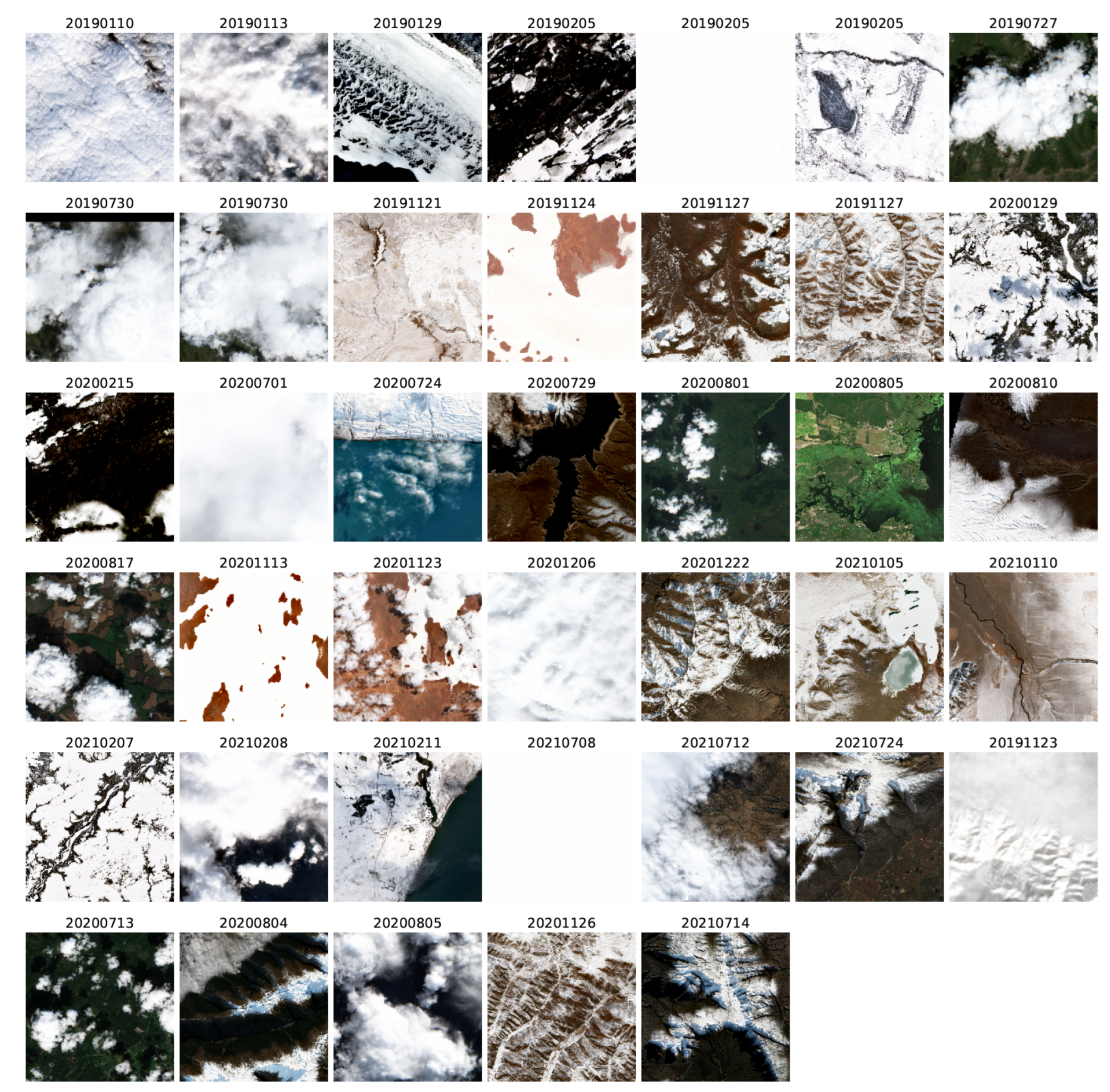
2.1. Satellite Image Collection

Sentinel-2 series satellites are selected to collect RS images in this study, which can be freely downloaded from Copernicus Open Access Hub, USGS EROS Archive, and Google Earth Engine. Their customized Multispectral Instrument (MSI) sensor can provide RS images with high spatial, spectral, and temporal resolutions. Regarding spectral information, there are a total of 12 spectral bands, including B1 (Aerosols), B2 (Blue), B3 (Green), B4 (Red), B5 (Red Edge 1), B6 (Red Edge 2), B7 (Red Edge 3), B8 (NIR), B8A (Red Edge 4), B9 (Water vapor), B11 (SWIR 1), and B12 (SWIR 2) [5]. In particular, B10 is omitted due to its lack of surface information. As shown in

Table 1. Band information of Sentinel-2A/B satellite.

Band No.	Characteristic	Wavelength ($\mathsf{\mu }$m)	Resolution (m)
1	Coastal Aerosol	0.443	60
2	Blue	0.490	10
3	Green	0.560	10
4	Red	0.665	10
5	Near Infrared (Red Edge 1)	0.705	20
6	Near Infrared (Red Edge 2)	0.740	20
7	Near Infrared (Red Edge 3)	0.783	20
8	Near Infrared (NIR)	0.842	10
8A	Near Infrared (Red Edge 4)	0.865	20
9	Water Vapor	0.945	60
10	Cirrus	1.375	60
11	Shortwave Infrared (SWIR 1)	1.610	20
12	Shortwave Infrared (SWIR 2)	2.190	20

, three levels of spatial resolution are available, where Band1, Band9, and Band10 are 60 m; Band8A, Band11, and Band12 are 20 m; and Band2, Band3, Band4, and Band8 are 10 m, meeting the requirements of various applications. A Sentinel-2 Level-2A product is directly utilized in this research rather than a Level-1C product because Level-2A is capable of offering Orthoimage Bottom Of Atmosphere (BOA)-corrected reflectance information. Moreover, the Level-2A product has a scene classification map composed of cloud and snow probabilities at 60 m resolution achieved via the Sen2Cor algorithm [12]. The dataset collected in this research includes 40 different Sentinel-2 scenes across the globe covering different continents (six continents except Antarctia) and years (2019, 2020, and 2021), months, and land-cover classes.

2.2. Data Labeling

This research aims to develop a novel method for snow/cloud classification via satellite images, so a proper method to label different objects is important. As mentioned in our previous work [12], a large diversity of scenes are needed to cover different continents, years, months, and land-cover classes (see Figure 2 for the retrieved dataset). There are a total of three classes labeled by human experts, including snow, cloud, and background. Based on the labeling process and satellite images, the pixel-label process was carried out in QGIS software with the help of its Semi-Automatic Classification Plugin, where the label images are displayed in Figure 3. It is noted that, to best separate the snow pixels from cloud pixels, not only RGB band images but also other false-color RGB images are drawn. Please refer to [12] for more details of the labeling process, and the labeled dataset is openly accessible for deep learning and satellite RS community. In our work, a total of 40 images are first collected via Sentinel-2 satellite, followed by manual labeling. The dataset is divided into training set with the size of 34 images, and the remaining 6 scenes constitute testing set. In addition, among the 12 bands in the Sentinel-2 Level-2A product, we select four bands data, namely B2, B11, B4, and B9, for the latter model’s training and classification [12]. It is notable that for better feature learning of band information, different bands are re-shaped into the same resolution of 10 m.

3. Methodology

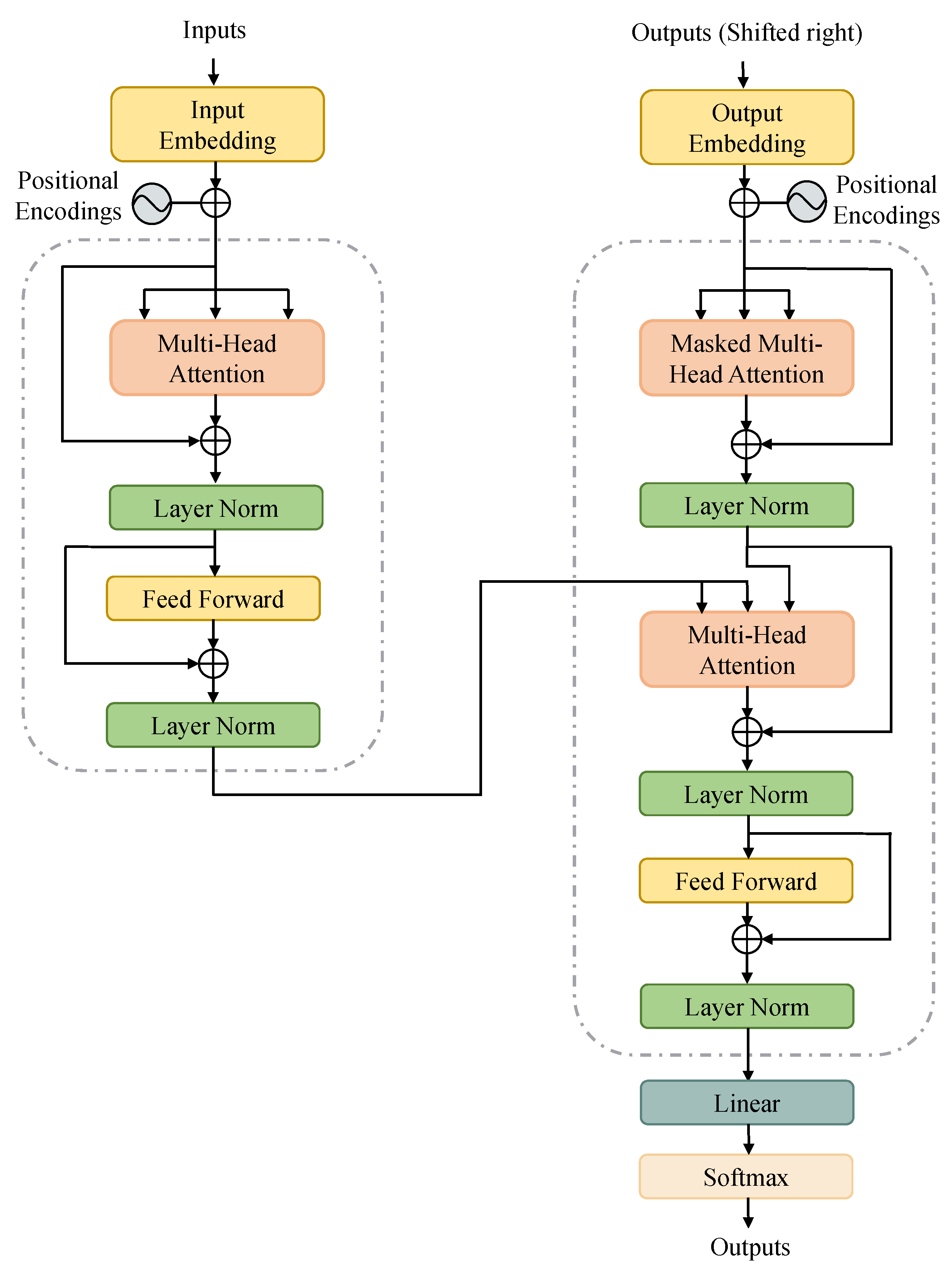
3.1. A Brief Review of Transformer

Transformer network [30], one of the the main architectures for a variety of natural language processing (NLP) tasks, has attracted an ever-increasing research interest in computer vision community since the success of Vision Transformer (ViT) [31]. By overcoming the insufficient global information modeling ability of CNNs, Transformer has created new state-of-the-art results for many vision tasks. Built on top of self-attention mechanisms, Transformer could build long-distance dependencies among pixels, which is crucial to accurately discriminate two similar classes such as cloud and snow in this paper.

Before proposing the dual-flow architecture, a brief introduction of vanilla Transformer is first reviewed [30]. The vanilla Transformer network stacks two kinds of Transformer blocks: encoder and decoder (see Figure 4). ViT adopts the original Transformer structure from NLP with minor modifications. Taking flattened image patches as tokens via appropriate feature embeddings, ViT only stacks the encoder blocks of vanilla Transformer since there is no need to prevent leftward information flow in computer vision application. A standard Transformer block is composed of a multi-head self-attention (MHSA) block and a fully connected feed-forward network (FFN). The MHSA block is able to model global relations with the help of self-attention characteristics, while the FFN is utilized for linear transformation of feature representations, enhancing model non-linearity. Moreover, these sub-layers are connected by residual connections and layer normalization to avoid gradient vanishing. In particular, given a feature sequence as input, the output of the $n_{th}$$(n\in [1,2,\dots ,N\left]\right)$ Transformer layer is calculated using Equation (1):

$$\begin{array}{c}{x}_n^{\prime }=MHSA\left(LN\left(x_{n-1}\right)\right)+x_{n-1},\hfill \\ x_n=FFN\left(LN\left(x_n^{\prime }\right)\right)+x_n^{\prime }\hfill \end{array}$$

(1)

where $LN(\ast )$ is the layer normalization, and $x_n$ is the output of $n_{th}$ Transformer layer.

However, without strong local information extraction abilities of convolution operations, Transformers blocks are not capable of modeling local semantics efficiently. As a result, it is intuitive that integrating Transformers and CNNs could achieve a complementary performance, which is the main task and will be explored in this paper.

3.2. Overall Architecture of UCTNet

The overall architecture of the proposed UCTNet is shown in Figure 5, which is a well-designed U-shaped network using dual branch to extract image information and achieve refined segmentation. The proposed network consists of two main parts, including encoder and decoder. The encoder is composed of five stages, namely Stem, Enc1, Enc2, Enc3. and Enc4. In particular, four Enc blocks extract hierarchical features from shallow, fine stage (Enc1) to deep, coarse stage (Enc4). The decoder consists of five main blocks, Dec1, Dec2, Dec3, FIFM, and AIFM, providing two prediction results based on the multi-level appearance information from the encoder. It is worth mentioning that, all blocks except Stem in both encoder and decoder contain a CNN branch and a Transformer branch to enhance global information awareness of network while retaining local details. The green and orange arrows in this architecture represent CNN and Transformer branches, respectively. C and D refer to the numbers of feature map channels and sequence feature dimensions in CNN and Transformer branches. Furthermore, H and W denote the height and width of the input image. Global perception capability of CNN branch is reinforced by the global contexts of Transformer branch. Similarly, local features from CNN branch are fed back to Transformer branch simultaneously, alleviating the issue of lack of spatial local information in Transformer branch.

The details of the encoder design are as follows. The encoder of UCTNet is divided into 5 stages to extract shallow spatial information and deep semantic information, including one Stem block and four Enc blocks, namely Enci ($i=1,\dots ,4$). The Stem module used to extract local features is a $7\times 7$ convolution with a stride of 2, followed by a Batch Normalization (BN) layer and a ReLU activation function. Enc1 uses a $1\times 1$ convolution and a Patch Embed process to generate the 2D and 3D features for CNN and Transformer branches. In Patch Embed process, we use a $1\times 1$ convolution to change the channel numbers to D and then flatten the feature map to a sequence of size $HW/4\times D$. After that, we use CTIM (detailed in Section 3.3) to make full use of CNN branch and Transformer branch information since CNN branch provides local feature and location information for the Transformer branch, and the Transformer branch provides global context information for the CNN branch. Other Enc stages (Enc2, Enc3, and Enc4) have the same data processing operations. In particular, the input of CNN branch in each stage has a size of $H/2^{i-1}\times W/2^{i-1}\times 2^{i-2}C$ ($i=2,3,4$), and it passes through C-Down to change features sizes. In C-Down process, we use a maximum pooling to reduce the resolution size by four times and a $1\times 1$ convolution to double the number of channels. At the same time, we adopt T-Down (patch merging in [27]) to convert the Transformer branch sequence characteristics from $HW/2^i\times 2^{i-2}D$ to $HW/2^{2i}\times 2^{i-1}D$. Then, the two branch features are sent to CTIM for feature extraction and fusion.

After encoder processing, the obtained hierarchical features are sent to decoder for dimension reduction and resolution restoration. The proposed decoder is composed of five blocks, including Decj, FIFM (detailed in Section 3.4), and AIFH (detailed in Section 3.5), where $j=1,2,3$. As presented in Figure 5, all of the Dec blocks share the same architecture, including CTIM module, C-Up, and T-Up operations, processing the features from encoders in two branches. In addition, we utilize skip connections to combine encoder features in the decoder, relieving the missing semantic information during encoder downsampling operations. In particular, for C-Up process in Deci blocks, we use bilinear interpolation to achieve a resolution conversion from $H/2^{5-j}\times W/2^{5-j}$ to $H/2^{4-j}\times W/2^{4-j}$, and the number of input channels is reduced from $2^{4-j}C$ to $2^{3-j}C$ via a $1\times 1$ convolution. Then, the C-Up output is concatenated with the feature map generated via the CNN branch of Enc($4-j$) along the channel dimension. After that, another $1\times 1$ convolution is utilized to restore the channel of integrated feature map to the previous size before skip connection. In Transformer branch, T-Up (patch expanding in [32]) changes the input sequence size from $HW/4^{5-j}$ to $HW/4^{4-j}$ firstly. Similarly, the T-Up output is concatenated with the sequence characteristic generated via the Transformer branch in Enc($4-j$) along the channel dimension, and a linear layer is used to divide the number of tokens into half. After dual-flow feature restoration, the results of these two branches are sent to CTIM for effective fusion. Finally, a well-designed FIFM integrates the outputs of two branches in Dec3 to obtain the final segmentation prediction of size $H\times W\times 3$ (note: 3 refers to the number of categories, including the background). In addition, we add AIFH in the outputs of Dec2 to generate another prediction result. These two prediction results are both utilized for better feature learning capability of the proposed model, enhancing its ability to segment the details of snow and clouds.

3.3. CNN and Transformer Integration Module Design

The structure of fusion module, namely CTIM is presented in Figure 6. CTIM uses a parallel structure of CNN branch and Transformer branch to leverage local features and global representations. In particular, CNN and Transformer branches pass through Conv_Block and Trans_Block, respectively. Then, the output features of one branch are transferred to the other branch for information fusion. For better integration of these two branches, we proposed two fusion methods in our model, including a complex way and a simple way. Most CTIMs adopt the simple way presented in Figure 6a, using only dimensional conversion (reshape or flatten) to bridge CNN and Transformer. In addition, the complex one is only used in Enc3 and Enc4 stages, and its structure are shown in Figure 6b,c. In complex way for two-branch fusion, a $3\times 3$ depth-wise convolution or a linear layer is applied to obtain the pixel-wise weights and then scaled via a sigmoid function. By assigning pixel-wise weights to the input before dimensional conversion, the complex way is capable of achieving the integration of deep features. After data fusion, CNN and Transformer branches pass through another Conv_Block and Trans_Block, obtaining outputs with the same dimensions as the input features. As the core module in the proposed dual-flow network, CTIM not only constructs the global context dependency but also enriches the local detail information, assisting model to segment snow and cloud accurately. The details of CNN and Transformer branches in CTIM are described as follows.

3.3.1. CNN Branch in CTIM

CNN branch mainly consists of two bottleneck blocks (Conv_Block). Following the definition in ResNet [33], a bottleneck block contains $1\times 1$ convolution, $3\times 3$ spatial convolution, batch normalization (BN), and Relu activation function. In addition, a designed residual connection is used to accelerate model convergence. In order to make up for the lack of CNN’s global information modeling ability, the outputs of Conv_Block1 and Trans_Block1 are fused. Before fusion, dimensional conversion is first carried out by reshaping the output of Trans_Block1 from $L_i\times D_i$ to $H_i\times W_i\times D_i$. Then, the converted feature from Transformer branch is concatenated with the feature map generated via Conv_Block1 in the channel dimension. After a $1\times 1$ convolution, the combined feature map of size $H_i\times W_i\times (C_i+D_i)$ has a channel dimension reduction from $C_i+D_i$ to $C_i$. Finally, the feature map is sent to Conv_Block2 to obtain the output of CNN branch with the size of $H_i\times W_i\times C_i$. With the help of convolution kernels sliding over feature maps, CNN branch could extract fine-detailed local features. In addition, by constructing the aforementioned fusion of Transformer branch information, the crucial context information for better classification performance could also be fully utilized.

3.3.2. Transformer Branch in CTIM

Similarly, the Transformer branch is composed of two Transformer blocks (Trans_Block). It is worth mentioning that to reduce computational complexity, we replace the original MHSA with an Efficient Multi-head Self-Attention (EMSA), which is proposed in [27]. Each Trans_Block consists of layer normalization (LN), EMSA, residual connections, and feed-forward network (FFN). Similar to CNN branch, the Transformer branch fuses the output of Trans_Block1 with the local feature representations from Conv_Block1. In particular, the output of Conv_Block1 is first flattened from $H_i\times W_i\times C_i$ to $L_i\times C_i$ and then concatenated with the sequence feature generated via Trans_Block1 in the channel dimension. We utilize a linear projection to reduce the integrated feature map dimension from size $L_i\times (C_i+D_i)$ to $L_i\times D_i$. Finally, the feature map passes through Trans_Block2 to obtain the Transformer branch output. By introducing the Transformer structure, the network enhances the ability to extract global information features. Moreover, in Transformer branch design, we discard the original location encoding as the proposed architecture could obtain the location information and local features from CNN branch, thus avoiding the limitation of the fixed and inflexible input size when using location encoding. To be more clear, the Transformer branch can be calculated using Equation (2)

$$\begin{array}{c}{\widehat{t}}_{i_1}=EMSA\left(LN\left(t_{i_1}\right)\right)+t_{i_1},\hfill \\ t_{i_1}^{\prime }=FFN\left(LN\left({\widehat{t}}_{i_1}\right)\right)+{\widehat{t}}_{i_1},\hfill \\ t_{i_2}=f\left(Concat(t_{i_1}^{\prime },{\tilde{c}}_{i_1})\right),\hfill \\ {\widehat{t}}_{i_2}=EMSA\left(LN\left(t_{i2}\right)\right)+t_{i_2},\hfill \\ t_{i_2}^{\prime }=FFN\left(LN\left({\widehat{t}}_{i_2}\right)\right)+{\widehat{t}}_{i_2}\hfill \end{array}$$

(2)

where i represents the $i_{th}$ stage, and $n\in 1,2$ means which Trans_Block the variable is related to. $t_{i_n}$ denotes the input of Trans_Blockn, and ${\widehat{t}}_{i_n}$ is the output of the EMSA in Trans_Blockn. $t_{i_n}^{\prime }$ denotes the output of Trans_Blockn, ${\tilde{c}}_{i_1}$ is the flattened output of Conv_Block1, $LN(\ast )$ represents the layer normalization, and $x_n$ is the output of n-th Transformer layer. $f(\ast )$ is the $1\times 1$ convolution for dimension reduction.

3.4. Final Information Fusion Module (FIFM) Design

As presented in Figure 7, the final information fusion module (FIFM) is proposed to fuse the CNN and Transformer branch outputs and obtain the final segmentation results. Both branch features (CNN and Transformer branches) pass through a linear layer and a $1\times 1$ convolution, respectively. The Transformer branch features are reshaped to the same spatial resolution as the CNN branch outputs, and these two branches results are concatenated in channel dimension. Then, a subsequent $1\times 1$ convolution is utilized to reduce the channels from $D+C$ to C, and the output is upsampled two times via bilinear interpolation to the size of original image. Finally, a $1\times 1$ class mapping convolution is used to obtain the segmentation prediction of size $H\times W\times 3$ (3 refers to the number of categories, including the background, snow, and cloud).

3.5. Auxiliary Information Fusion Head (AIFH) Design

The auxiliary information fusion head (AIFH), as shown in Figure 8, is designed additionally for enhancing feature representations of stage Dec2. Similar to FIFM, we concatenate Transformer branch and CNN branch in channel dimension. Furthermore, a subsequent $1\times 1$ convolution is used to reduce the dimension from $D+C$ to C. Then, we use upsampling process followed by $1\times 1$ convolution operation twice to generate an auxiliary segmentation map, which is used for CE loss calculation together with the FIFM prediction map during model training, promoting the ability of feature learning in this model.

3.6. Loss Function Design

In the output of FIFM and AIFH, we calculate the Cross Entropy Loss (CEloss) as a training loss function, which is a natural choice for image segmentation. In particular, as presented Equation (3), CEloss is the sum of cross entropy terms for each pixel in the output images and ground truth, where $x_i$ denotes the predicted map, and $y_i$ means the labeled map.

$$\begin{array}{c}CELoss(x,y)=-\sum _{i=0}^n{y}_i\ast log\left(x_i\right)\hfill \end{array}.$$

(3)

3.7. Experimental Settings

Our proposed UCTNet is implemented on the PyTorch platform and trained with two high performance computing (HPC) resource NVIDIA RTX 2080 Ti GPUs. We trained our method for 120 epochs using AdamW strategy [34], with a cosine decay learning rate scheduler and 5 epochs of warm-up. An initial learning rate of $5\times {10}^5$, a weight decay of 0.01, a momentum of 0.9, and a batch size of 16 are used. Regarding parameter configuration of the UCTNet, we set C, D for the CNN and Transformer branches to 32. In the Transformer branch, the dimensional change rate of the linear layer in the MLP is set as 2, the number of EMSA heads in the four encoder stages (from Enc1 to Enc4) is set as 1, 2, 4, and 8, respectively. Meanwhile, the number of EMSA heads in the three decoder stages (from Dec1 to Dec3) is 4, 2, and 1, respectively. The reduction ratio of the EMSA from Enc1 to Enc4 is set to 8, 4, 2, and 1. Correspondingly, the reduction ratio of the EMSA from Dec1 to Dec3 is set to 1, 2, and 4.

3.8. Performance Metrics

We evaluate the segmentation performance quantitatively using five commonly-used metrics, including Precision, Recall, $F_1$ score, Accuracy (ACC), and Intersection over Union (IoU). These corresponding formulations can be seen in Equations (4)–(6).

$$\begin{array}{c}Precision={\displaystyle \frac{TP}{TP+FP}},Recall={\displaystyle \frac{TP}{TP+FN}},\hfill \end{array}$$

(4)

$$\begin{array}{c}ACC={\displaystyle \frac{TP+TN}{P+N}},IoU={\displaystyle \frac{TP}{TP+FP+FN}},\hfill \end{array}$$

(5)

$$\begin{array}{c}{F}_1=2\times {\displaystyle \frac{Precision\times Recall}{Precision+Recall}}\hfill \end{array}.$$

(6)

where P, N, T, and F are the abbreviations of positive, negative, true, and false pixels in the prediction map, respectively. Particularly, True Positive ($TP$) denotes the correctly predicted positive values; False Positive ($FP$) is the value where actual class is negative, and the predicted class is positive; False Negative ($FN$) means the scenario where the actual class is positive, but the predicted class is negative; True Negative ($TN$) is the truly predicted negative values. mIoU denotes the average of all categories of the IoU, which describes the coincidence degree of labels and prediction outputs. We select mIoU as the main evaluation criterion in our experiments since it is one of the most popular metric in segmentation tasks. If the class is not indicated specifically, all metrics are the average of the three classes’ results.

4. Results

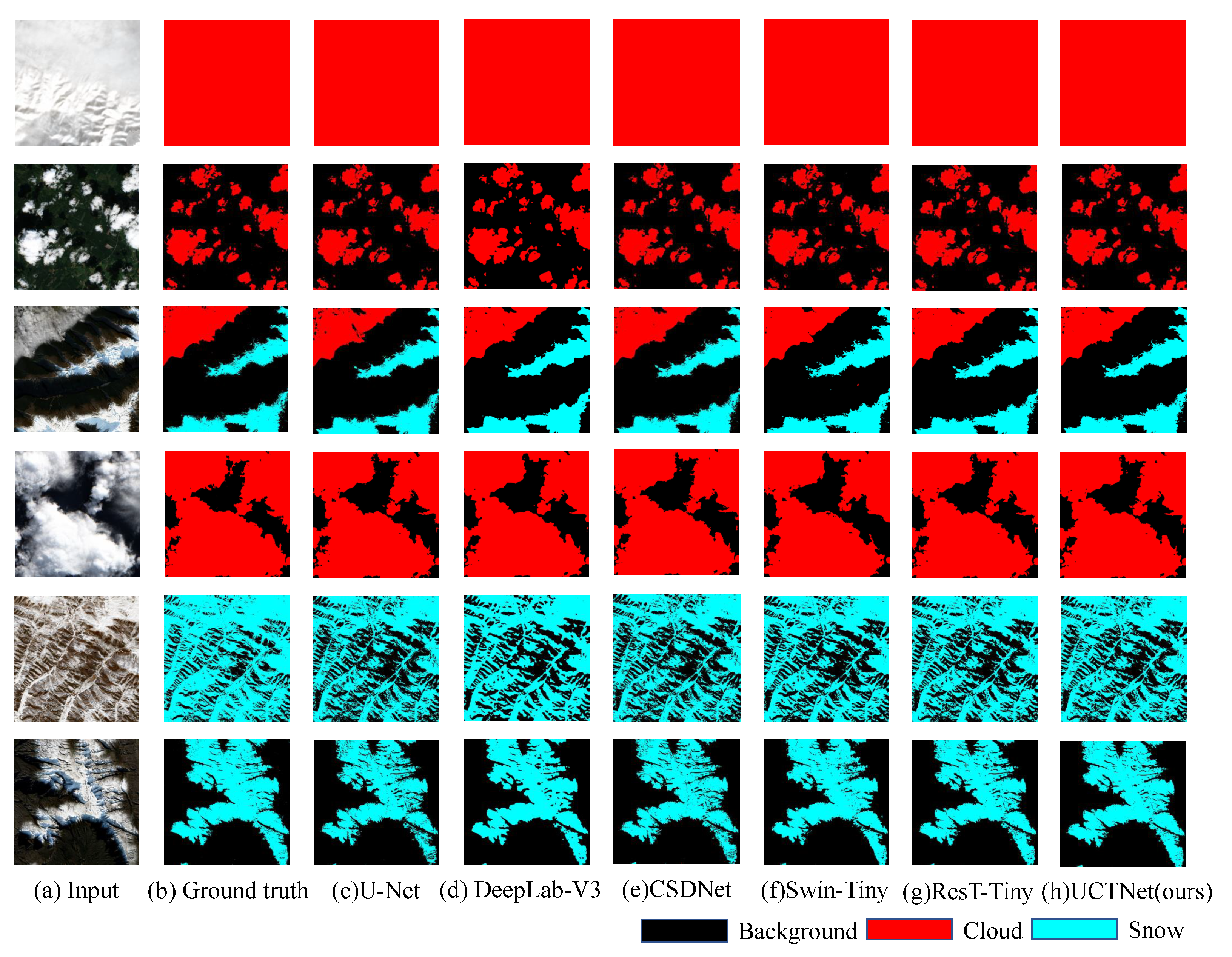
4.1. Quantitative and Qualitative Result Analysis

First, we illustrate the performance of the proposed UCTNet on the previously stated snow/cloud dataset. As shown in

Table 2. Performance comparison with current popular methods, where the best performance is highlighted in bold.

Methods	Multiscale Testing	Params (M)	Precision (%)	Recall (%)	F1 (%)	ACC (%)	mIoU
U-Net	✓	13.40	95.74	92.97	94.03	94.58	88.91
DeepLab-V3	✓	16.42	95.41	93.65	94.38	94.84	89.51
CSDNet	✓	8.66	96.10	93.67	94.63	95.17	89.97
Swin-Tiny	✓	29.25	95.10	93.10	93.92	94.35	88.67
ResT-Tiny	✓	11.30	95.65	93.70	94.50	94.92	89.70
UCTNet (ours)	✓	3.93	96.24	94.68	95.35	95.72	91.21

, a variety of methods are used for the performance comparison, including commonly used segmentation methods and the specially designed snow and cloud detection method (i.e., CSD-Net [35]). Segmentation methods could be categorized into CNN-based methods (i.e., U-Net [36] and DeepLab-V3 [37]) and recently proposed Transformer-based networks (i.e., ResT-Tiny [38] and Swin-Tiny [27]). In addition, multiscale testing is also used as a common trick for performance improvement, and the results are listed to have a comparison with other popular models. It is obvious that our proposed method UCTNet is able to achieve the best performance in terms of all evaluation metrics, where Precision, Recall, F1, ACC, and mIoU are 96.24%, 94.68%, 95.35%, 95.72%, and 91.21%, respectively.

Compared with CNN-based networks, namely U-Net and DeepLab-V3, the mIoU of UCTNet is increased by 2.30% and 1.70%. Moreover, these two Transformer-based methods require loading pre-trained weight and position coding, while the Transformer branch in our model could get rid of them with the CNN branch providing the required local feature and location information. Therefore, as presented in the results of the last three lines, there is a 2.54% and 1.51% increase in the mIoU compared with the two Transformer-based methods. As a result, UCTNet could combine the advantages of CNN and Transformer, thus enhancing the feature extraction ability. It does not require pre-trained weights, being flexibly adjusted to different input sizes without the restrictions of position coding. Such a conclusion can also be seen from a qualitative visualization in Figure 9. It can be found that the proposed method is much better than other approaches in segmentation details for the snow/cloud classification task. It is noticed that the multiscale testing strategy is only used in this section. The following comparisons with different modules are with no multiscale testing strategy.

4.2. Exploration on the Effectiveness of Two Branches Architecture

In order to verify the effectiveness of the proposed dual-flow architecture, we make an ablation study to compare the results of the CNN branch (Only CNN), the Transformer branch (Only Trans), and the dual-flow architecture (CNN+Trans) in the proposed UCTNet. The results are shown in

Table 3. Exploration on the effectiveness of the two-branch architecture.

Methods	C → T	T → C	Precision (%)	Recall (%)	F1 (%)	ACC (%)	mIoU (%)
Only CNN	-	-	95.47	92.56	93.66	94.21	88.28
Only Trans	-	-	95.48	93.81	94.51	94.9	89.72
CNN + Trans			95.3	93.06	93.96	94.39	88.76
		✓	95.71	93.48	94.37	94.83	89.49
	✓		95.42	93.15	94.05	94.52	88.93
	✓	✓	95.94	94.27	94.97	95.37	90.56

, where C → T and T → C refer to fusing the features extracted via CNN in the Transformer branch and fusing the features extracted via Transformer in the CNN branch. Taking mIoU as the main evaluation reference, it can be first seen that a single Transformer branch could obtain 89.72% mIoU, which is higher than the result of single CNN branch, demonstrating the superior performance of Transformer architecture in this particular task. However, by using the dual-flow architecture, the network could increase the mIoU score up to 90.56%, demonstrating that CNNs and Transformers can complement each other to improve model performance.

Moreover, as shown in the last four lines, we conduct further experiments to evaluate the necessity of the mutual integration of these two branches. Compared with the dual-flow structure without feature fusion, the utilization of T → C and C → T structure in two-branch fusion increases the mIoU scores by 0.73% and 0.17% respectively, showing that information integration is significant for CNN and Transformer branch performance. It is notable that the results of only using the Transformer branch is even better than these two branches structure for one-way fusion (T → C) and no fusion methods. This is because these two branch outputs in Dec2 and Dec3 need to be fused in the FIFM and AIFH modules to generate the final prediction map, but the large difference between branch features caused by no fusion or one-way fusion in the previous CTIM makes it difficult for these two modules to segment precisely. As a result, we can conclude that the dual-flow structure is capable of combining CNN and Transformer information for better fusion, and the CTIM fusion block makes full use of local and global features, effectively improving the final segmentation accuracy.

4.3. Exploration on Location Setting of the Complex Ctim

An ablation study is conducted to explore the adequate location of the complex CTIM. We select different types of CTIM (the simple or the complex one) for seven fusion modules at the corresponding positions of encoders and decoders to generate features, including local details and global contexts. For the scores in

Table 4. Ablation study on the location setting of the complex CTIM.

Methods	Position of the Complex CTIM			Precision (%)	Recall (%)	F1 (%)	ACC (%)	mIoU (%)
	①	②	③
UCTNet				95.46	93.4	94.23	94.75	89.28
			✓	95.66	93.64	94.46	94.93	89.67
		✓		95.94	94.27	94.97	95.37	90.56
		✓	✓	95.78	93.92	94.69	95.14	90.07
	✓			95.57	92.92	93.94	94.52	88.79
	✓		✓	95.57	93.22	94.15	94.65	89.12
	✓	✓		95.54	93.79	94.52	94.94	89.75
	✓	✓	✓	95.36	93.12	94.01	94.53	88.89

, ①, ②, and ③ represent Enc1 and Enc2; Enc3 and Enc4; and Dec1, Dec2, and Dec3, respectively. “” means that the simple CTIM is replaced by the complex version in this position. The details of a simple or complex CTIM are introduced in Section 3.3. As presented in the first line of Table 4, using simple CTIM in all stages to fuse features could not leverage the full advantages of the CNN and Transformer, which only reaches a score of 89.28% in the mIoU. When using the complex CTIM to obtain a better integration of information, lines 5, 6, and 8 show that the performance may not be improved if the complex CTIM is placed in an arbitrary position, resulting in an even worse result. Compared with the results obtained via the structure using only simple CTIM in line 1, selecting complex CTIM in ② could increase the mIoU by 1.28%, which is also the most suitable settings for CTIM. However, choosing the complex CTIM in both ② and ③ leads to a 0.49% decrease in the mIoU score shown in line 4. The comparisons indicate that using the complex CTIM in the encoder deep stages (Enc3 and Enc4) is enough for network to make the most use of dual-flow information, which could also be demonstrated in the results of line 5 and line 7. It shows that the complex CTIM used in Enc3 and Enc4 and Dec1, Dec2, and Dec3 could not make further improvements than the complex connection used in Enc3 and Enc4.

4.4. Exploration on Position Encoding of the Transformer Branch

Next, we conduct an ablation experiment to analyze the impact of different positional encodings (PEs) used for the Transformer branch in CTIM. Four kinds of positional encoding strategies are utilized for comparisons, including without PE (w/o PE), absolute PE, learnable PE, and convolutional PE (using a pixel-wise attention module to encode positions [38]). The experimental results are shown in

Table 5. Ablation study on different designs for positional encodings of the Transformer branch.

Methods	Precision (%)	Recall (%)	F1 (%)	ACC (%)	mIoU
absolute PE	95.84	94.21	94.9	95.32	90.44
learnable PE	95.49	93.43	94.27	94.75	89.33
convolutional PE	95.66	93.56	94.41	94.88	89.57
w/o PE	95.94	94.27	94.97	95.37	90.56

. It can be found that using CTIM without PE could achieve the best scores of the four evaluation metrics and adding the absolute PE leads to a slight drop in the results. Meanwhile, it can be observed that there is a considerable gap in the performance between the networks using two kinds of learnable PE (learnable PE and convolutional PE) and the network without PE, dropping by 1.23% and 0.99% mIoU, respectively. In a word, the accuracy of the model is reduced after adding PE. As a consequence, it is believed that this is because the CNN branch could obtain local features and position information, making up for PE in the traditional Transformer model. Therefore, the Transformer branch in our model could discard PE, avoiding the limitation of fixed input size and achieving a better capability of spatial feature extraction.

4.5. Exploration on the Effectiveness of AIFH

In this paper, we additionally proposed AIFM to integrate the dual-branch outputs of Dec2, improving the feature integration and feature modeling capabilities of UCTNet. As seen in

Table 6. Ablation study on the effectiveness of AIFH.

Methods	AIFH	Precision (%)	Recall (%)	F1 (%)	ACC (%)	mIoU
UCTNet		95.89	94.08	94.83	95.25	90.31
	✓	95.94	94.27	94.97	95.37	90.56

, with the help of AIFH, our model could increase the Precision, Recall, F1, ACC, and mIoU scores by 0.05%, 0.19%, 0.14%, 0.14%, and 0.25% respectively, showing that the application of the auxiliary head to the two-branch architecture could improve the performance to some extent.

5. Discussion

The dual-flow UCTNet presented in Section 3 show better performance than previous methods in terms of Precision, Recall, $F_1$ score, ACC, and mIoU on the collected snow/cloud dataset. Taking mIoU as the main evaluation criterion, the proposed UCTNet increases by 2.30% and 1.70% compared with CNN-based networks (i.e., U-Net and DeepLab-V3). Moreover, our method is 2.54% and 1.51% higher than previous Transformer-based approaches (i.e., ResT-Tiny and Swin-Tiny). By leveraging the local and global feature modeling ability of CNNs and Transformers, our UCTNet also increases the mIoU by 1.24% than the specially designed snow and cloud detection method (i.e., CSD-Net). In addition, extensive ablation experiments are conducted on the two-branch architecture, local–global fusion approach, position encoding for the Transformer branch, and the well-designed AIFH, further verifying the superiority of the proposed method.

There are still some issues worthy of investigation when the proposed method is utilized in practical scenarios. For example, the spatial resolution of the Sentinel-2 satellite is approximately 10 m. Therefore, certain pixels (especially those at the boundaries of different classes) actually constitute mixed spectral information of several surface classes. Furthermore, extremely small proportions of clouds and snow coverage within pixels cannot be effectively identified. Consequently, the classification performance concerning the aforementioned issues yields unsatisfactory outcomes. Our method can solve these problems when training on datasets with elevated spatial resolution.

6. Conclusions and Future Work

This paper investigates the challenging task of snow/cloud classification, which is important for land-cover classification and precision agriculture. A dual-flow U-shaped framework named UCTNet is proposed to integrate CNNs and Transformers in discriminating snow and clouds. In particular, the CTIM module is designed to integrate the CNN branch and Transformer branch to take advantage of local features and global representations concurrently; FIFM is proposed to fuse CNN and Transformer branch outputs and obtain the final segmentation results. Moreover, the AIFH module is designed additionally for enhancing feature representations of stage Dec2. All of the methods are validated on a real dataset collected via Sentinel-2 satellite for snow/cloud classification. For performance evaluation, the proposed algorithm is compared to various CNN- and Transformer-based methods, yielding the best segmentation performance in terms of accuracy (95.72%) and mIoU score (91.21%) while with the smallest model size (3.93 M). In addition, these different modules are also verified in the ablation study to explore which kind of combination/module is the best for our particular problem.

Although the results in this study are quite promising, there is still room for further development. First, the dataset limits the performance of the proposed model. An entire dataset with more labeled samples and more diverse textures of snow and clouds could be established for a highly accurate evaluation. Meanwhile, a strong feature integration module is expected to be designed for better fusion in this proposed architecture.

References

1. Munawar, H.S.; Ullah, F.; Qayyum, S.; Khan, S.I.; Mojtahedi, M. Uavs in disaster management: Application of integrated aerial imagery and convolutional neural network for flood detection. Sustainability 2021, 13, 7547. [Google Scholar] [CrossRef]
2. Wang, C.; Wang, Y.; Wang, R.; Zheng, P. Modeling and evaluating land-use/land-cover change for urban planning and sustainability: A case study of Dongying city, China. J. Clean. Prod. 2018, 172, 1529–1534. [Google Scholar] [CrossRef]
3. Cai, G.; Ren, H.; Yang, L.; Zhang, N.; Du, M.; Wu, C. Detailed urban land use land cover classification at the metropolitan scale using a three-layer classification scheme. Sensors 2019, 19, 3120. [Google Scholar] [CrossRef] [PubMed]
4. Shi, H.; Chen, L.; Bi, F.K.; Chen, H.; Yu, Y. Accurate urban area detection in remote sensing images. IEEE Geosci. Remote Sens. Lett. 2015, 12, 1948–1952. [Google Scholar] [CrossRef]
5. Zhang, T.; Su, J.; Xu, Z.; Luo, Y.; Li, J. Sentinel-2 satellite imagery for urban land cover classification by optimized random forest classifier. Appl. Sci. 2021, 11, 543. [Google Scholar] [CrossRef]
6. Gannon, C.S.; Steinberg, N.C. A global assessment of wildfire potential under climate change utilizing Keetch-Byram drought index and land cover classifications. Environ. Res. Commun. 2021, 3, 035002. [Google Scholar] [CrossRef]
7. Kumar, M.; Fadhil Al-Quraishi, A.M.; Mondal, I. Glacier changes monitoring in Bhutan High Himalaya using remote sensing technology. Environ. Eng. Res. 2020, 26, 190255. [Google Scholar] [CrossRef]
8. Kussul, N.; Lavreniuk, M.; Skakun, S.; Shelestov, A. Deep learning classification of land cover and crop types using remote sensing data. IEEE Geosci. Remote Sens. Lett. 2017, 14, 778–782. [Google Scholar] [CrossRef]
9. Zhang, T.X.; Su, J.Y.; Liu, C.J.; Chen, W.H. Potential bands of sentinel-2A satellite for classification problems in precision agriculture. Int. J. Autom. Comput. 2019, 16, 16–26. [Google Scholar] [CrossRef]
10. Zhang, Y.; Rossow, W.B.; Lacis, A.A.; Oinas, V.; Mishchenko, M.I. Calculation of radiative fluxes from the surface to top of atmosphere based on ISCCP and other global data sets: Refinements of the radiative transfer model and the input data. J. Geophys. Res. Atmos. 2004, 109, 19105. [Google Scholar] [CrossRef]
11. Yin, M.; Wang, P.; Ni, C.; Hao, W. Cloud and Snow Detection of Remote Sensing Images Based on Improved Unet3. Sci. Rep. 2022, 12, 14415. [Google Scholar] [CrossRef]
12. Wang, Y.; Su, J.; Zhai, X.; Meng, F.; Liu, C. Snow coverage mapping by learning from sentinel-2 satellite multispectral images via machine learning algorithms. Remote Sens. 2022, 14, 782. [Google Scholar] [CrossRef]
13. Su, J.; Yi, D.; Su, B.; Mi, Z.; Liu, C.; Hu, X.; Xu, X.; Guo, L.; Chen, W.H. Aerial Visual Perception in Smart Farming: Field Study of Wheat Yellow Rust Monitoring. IEEE Trans. Ind. Inform. 2020, 17, 2242–2249. [Google Scholar] [CrossRef]
14. Zhu, Z.; Wang, S.; Woodcock, C.E. Improvement and expansion of the Fmask algorithm: Cloud, cloud shadow, and snow detection for Landsats 4–7, 8, and Sentinel 2 images. Remote Sens. Environ. 2015, 159, 269–277. [Google Scholar] [CrossRef]
15. Irish, R.R.; Barker, J.L.; Goward, S.N.; Arvidson, T. Characterization of the Landsat-7 ETM+ automated cloud-cover assessment (ACCA) algorithm. Photogramm. Eng. Remote Sens. 2006, 72, 1179–1188. [Google Scholar] [CrossRef]
16. Zhu, Z.; Woodcock, C.E. Automated cloud, cloud shadow, and snow detection in multitemporal Landsat data: An algorithm designed specifically for monitoring land cover change. Remote Sens. Environ. 2014, 152, 217–234. [Google Scholar] [CrossRef]
17. Stillinger, T.; Roberts, D.A.; Collar, N.M.; Dozier, J. Cloud masking for Landsat 8 and MODIS Terra over snow-covered terrain: Error analysis and spectral similarity between snow and cloud. Water Resour. Res. 2019, 55, 6169–6184. [Google Scholar] [CrossRef] [PubMed]
18. Bai, T.; Li, D.; Sun, K.; Chen, Y.; Li, W. Cloud detection for high-resolution satellite imagery using machine learning and multi-feature fusion. Remote Sens. 2016, 8, 715. [Google Scholar] [CrossRef]
19. Nijhawan, R.; Raman, B.; Das, J. Meta-classifier approach with ANN, SVM, rotation forest, and random forest for snow cover mapping. In Proceedings of the 2nd International Conference on Computer Vision & Image Processing, Roorkee, India, 9–12 September 2017; Springer: Berlin/Heidelberg, Germany, 2018; pp. 279–287. [Google Scholar]
20. Ghasemian, N.; Akhoondzadeh, M. Integration of VIR and thermal bands for cloud, snow/ice and thin cirrus detection in MODIS satellite images. In Proceedings of the Third International Conference on Intelligent Decision Science, Tehran, Iran, 16–18 May 2018; pp. 1–37. [Google Scholar]
21. Foga, S.; Scaramuzza, P.L.; Guo, S.; Zhu, Z.; Dilley, R.D., Jr.; Beckmann, T.; Schmidt, G.L.; Dwyer, J.L.; Hughes, M.J.; Laue, B. Cloud detection algorithm comparison and validation for operational Landsat data products. Remote Sens. Environ. 2017, 194, 379–390. [Google Scholar] [CrossRef]
22. Wang, L.; Chen, Y.; Tang, L.; Fan, R.; Yao, Y. Object-based convolutional neural networks for cloud and snow detection in high-resolution multispectral imagers. Water 2018, 10, 1666. [Google Scholar] [CrossRef]
23. Mohapatra, M.; Gupta, P.K.; Nikam, B.R.; Thakur, P.K. Cloud segmentation in Advanced Wide Field Sensor (AWiFS) data products using deep learning approach. J. Geomat. 2022, 16, 33–44. [Google Scholar]
24. Zhan, Y.; Wang, J.; Shi, J.; Cheng, G.; Yao, L.; Sun, W. Distinguishing cloud and snow in satellite images via deep convolutional network. IEEE Geosci. Remote Sens. Lett. 2017, 14, 1785–1789. [Google Scholar] [CrossRef]
25. He, J.; Zhao, L.; Yang, H.; Zhang, M.; Li, W. HSI-BERT: Hyperspectral image classification using the bidirectional encoder representation from transformers. IEEE Trans. Geosci. Remote Sens. 2019, 58, 165–178. [Google Scholar] [CrossRef]
26. Yu, Y.; Jiang, T.; Gao, J.; Guan, H.; Li, D.; Gao, S.; Tang, E.; Wang, W.; Tang, P.; Li, J. CapViT: Cross-context capsule vision transformers for land cover classification with airborne multispectral LiDAR data. Int. J. Appl. Earth Obs. Geoinf. 2022, 111, 102837. [Google Scholar] [CrossRef]
27. Liu, Z.; Lin, Y.; Cao, Y.; Hu, H.; Wei, Y.; Zhang, Z.; Lin, S.; Guo, B. Swin transformer: Hierarchical vision transformer using shifted windows. In Proceedings of the IEEE/CVF International Conference on Computer Vision, Montreal, BC, Canada, 10–17 October 2021; pp. 10012–10022. [Google Scholar]
28. Xu, Z.; Zhang, W.; Zhang, T.; Yang, Z.; Li, J. Efficient transformer for remote sensing image segmentation. Remote Sens. 2021, 13, 3585. [Google Scholar] [CrossRef]
29. Wang, L.; Li, R.; Duan, C.; Zhang, C.; Meng, X.; Fang, S. A novel transformer based semantic segmentation scheme for fine-resolution remote sensing images. IEEE Geosci. Remote Sens. Lett. 2022, 19, 1–5. [Google Scholar] [CrossRef]
30. Vaswani, A.; Shazeer, N.; Parmar, N.; Uszkoreit, J.; Jones, L.; Gomez, A.N.; Kaiser, Ł; Polosukhin, I. Attention is all you need. Adv. Neural Inf. Process. Syst. 2017, 30, 1–15. [Google Scholar] [CrossRef]
31. Dosovitskiy, A.; Beyer, L.; Kolesnikov, A.; Weissenborn, D.; Zhai, X.; Unterthiner, T.; Dehghani, M.; Minderer, M.; Heigold, G.; Gelly, S.; et al. An image is worth 16 × 16 words: Transformers for image recognition at scale. arXiv 2020, arXiv:2010.11929. [Google Scholar]
32. Cao, H.; Wang, Y.; Chen, J.; Jiang, D.; Zhang, X.; Tian, Q.; Wang, M. Swin-unet: Unet-like pure transformer for medical image segmentation. arXiv 2021, arXiv:2105.05537. [Google Scholar]
33. He, K.; Zhang, X.; Ren, S.; Sun, J. Deep residual learning for image recognition. In Proceedings of the IEEE Conference on Computer Vision and Pattern Recognition, Las Vegas, NV, USA, 27–30 June 2016; pp. 770–778. [Google Scholar]
34. Loshchilov, I.; Hutter, F. Decoupled Weight Decay Regularization. In Proceedings of the International Conference on Learning Representations, Vancouver, BC, Canada, 30 April–3 May 2018. [Google Scholar]
35. Zhang, G.; Gao, X.; Yang, Y.; Wang, M.; Ran, S. Controllably Deep Supervision and Multi-Scale Feature Fusion Network for Cloud and Snow Detection Based on Medium-and High-Resolution Imagery Dataset. Remote Sens. 2021, 13, 4805. [Google Scholar] [CrossRef]
36. Ronneberger, O.; Fischer, P.; Brox, T. U-net: Convolutional networks for biomedical image segmentation. In Proceedings of the International Conference on Medical Image Computing and Computer-Assisted Intervention, Munich, Germany, 5–9 October 2015; Springer: Berlin/Heidelberg, Germany, 2015; pp. 234–241. [Google Scholar]
37. Chen, L.C.; Papandreou, G.; Schroff, F.; Adam, H. Rethinking atrous convolution for semantic image segmentation. arXiv 2017, arXiv:1706.05587. [Google Scholar]
38. Zhang, Q.; Yang, Y.B. ResT: An efficient transformer for visual recognition. Adv. Neural Inf. Process. Syst. 2021, 34, 15475–15485. [Google Scholar]
Figure 1. Framework of snow/cloud classification research in this study.
Remotesensing 15 04213 g001
Figure 2. Visualization of all 40 scenes captured using Sentinel-2 satellite with scene captured date [12].
Remotesensing 15 04213 g002
Figure 3. Labeled classification maps of all 40 collected scenes. The three labeled classes are in different colors: black denotes background, red denotes cloud, and cyan denotes snow [12].
Remotesensing 15 04213 g003
Figure 4. Illustration of the vanilla Transformer architecture.
Remotesensing 15 04213 g004
Figure 5. Architecture of the proposed UCTNet by dual–flow approach.
Remotesensing 15 04213 g005
Figure 6. Structure of CTIM module to leverage local features and global representations.
Remotesensing 15 04213 g006
Figure 7. Structure of FIFM module to finally fuse CNN–Transformer branch information.
Remotesensing 15 04213 g007
Figure 8. The structure of AIFH module to enhance feature representations of stage Dec2.
Remotesensing 15 04213 g008
Figure 9. Visualization of segmentation results by different models.
Remotesensing 15 04213 g009