
Estimation of Coastal Wetland Soil Organic Carbon Content in Western Bohai Bay Using Remote Sensing, Climate, and Topographic Data

 ,
,  ,
,  , ,
, ,
Abstract
:
1. Introduction
2. Materials and Methods
2.1. Study Area
2.2. Soil Sampling and Analysis
2.3. Predictor Variables
2.3.1. Remote Sensing Variables and Processing

| Sources | Category | Variables | Calculation Formula | Literature |
|---|---|---|---|---|
| SAR images | Polarization backscattering coefficient | VV, VH | - | [32] |
| D | VV − VH | [32] | ||
| S | VV + VH | [32] | ||
| Q | VV/VH | [32] | ||
| DSR | (VV − VH)/(VV + VH) | |||
| optical images | Band reflectance | B2 (490 nm), B3 (560 nm) B4 (665 nm), B5 (705 nm) B6 (740 nm), B7 (783 nm) B8 (842 nm), B8A (865 nm) B11 (1610 nm), B12 (2190 nm) | − | [32] |
| NDVI | (B8 − B4)/(B8 + B4) | [33] | ||
| NDWI | (B3 − B8)/(B3 + B8) | [34] | ||
| Remote sensing indices | NDBI | (B11 − B8)/(B11 + B8) | [35] | |
| SAVI | 1.5 × (B8 − B4)/(B8 + B4 + 0.5) | [36] | ||
| RVI | [37] | |||
| DVI | B8 − B4 | [38] | ||
| EVI | 2.5 × (B8 − B4)/(B8 + 6 × B4 − 7.5 × B2 + 1) | [39] | ||
| BSI | 1 + ((B4 + B11) − (B8 + B2))/((B4 + B11) + (B8 + B2)) | [40] | ||
| NDRE1 | (B6 − B5)/(B6 + B5) | [41] | ||
| NDRE2 | (B7 − B5)/(B7 + B5) | [41] | ||
| CIRE1 | (B8/B5) − 1 | [42] | ||
| CIRE2 | (B8/B6) − 1 | [42] | ||
| CIRE3 | (B8/B7) − 1 | [42] | ||
| NDVIRE1 | (B8 − B5)/(B8 + B5) | [43] | ||
| NDVIRE2 | (B8 − B6)/(B8 + B6) | [43] | ||
| NDVIRE3 | (B8 − B7)/(B8 + B7) | [43] |
2.3.2. Environmental Variables
2.4. Boruta
2.5. Modeling Methods
2.5.1. Random Forest
2.5.2. Gradient Boosting Machine
2.5.3. Extreme Gradient Boosting
2.6. Model Performance Evaluation
3. Results
3.1. Model Performance Comparison
3.2. Relative Importance of Predictor Variables
3.3. Spatial Distribution Prediction of the CW-SOC Content
4. Discussion
4.1. Prediction Accuracy Comparison of Machine Learning Methods
4.2. Influence of Predictor Variables on CW-SOC Content Prediction
4.3. Spatial Distribution Characteristics of CW-SOC Content
5. Conclusions
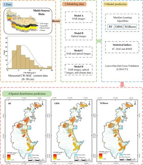
- (1)
- Combining SAR images and optical images can effectively improve the prediction accuracy of the model. After adding climate variables, the performance of the model is further improved, but the optimization effect is not obvious, and the prediction accuracy is only increased by 7% (RF), 6% (GBM), and 2.2% (XGBoost).
- (2)
- XGBoost method exhibits better prediction ability than the RF and GBM method. The optimal model is built using the XGBoost method, with the R2 as high as 0.730, and the MAE and RMSE as low as 0.554 g·kg−1 and 0.899 g·kg−1, respectively.
- (3)
- Remote sensing variables are the primary explanatory variables for predicting CW-SOC content, with optical images being the most prominent contributor, explaining more than 65% of the variability. The most important predictor variables for the RF, GBM, and XGBoost method were MARH (12.2%), DVI (18.1%), and B2 (37.6%), respectively.
- (4)
- CW-SOC content gradually increase from the coast to the inland. The CW-SOC content is lower in the south and north of the study area and higher in the central area. The mean value of CW-SOC content in Binhai New District is higher than those in Huanghua and Haixing.
Author Contributions
Funding
Data Availability Statement
Acknowledgments
Conflicts of Interest
References
- Rumpel, C.; Amiraslani, F.; Koutika, L.S.; Smith, P.; Whitehead, D.; Wollenberg, E. Put more carbon in soils to meet Paris climate pledges. Nature 2018, 564, 32–34. [Google Scholar] [CrossRef] [PubMed]
- Dharumarajan, S.; Kalaiselvi, B.; Suputhra, A.; Lalitha, M.; Vasundhara, R.; Kumar, K.S.A.; Nair, K.M.; Hegde, R.; Singh, S.K.; Lagacherie, P. Digital soil mapping of soil organic carbon stocks in Western Ghats, South India. Geoderma Reg. 2021, 25, e00387. [Google Scholar] [CrossRef]
- Fernández-Martínez, M.; Peñuelas, J.; Chevallier, F.; Ciais, P.; Obersteiner, M.; Rödenbeck, C.; Sardans, J.; Vicca, S.; Yang, H.; Sitch, S.; et al. Diagnosing destabilization risk in global land carbon sinks. Nature 2023, 615, 848–853. [Google Scholar] [CrossRef]
- Mao, D.; Luo, L.; Wang, Z.; Wilson, M.C.; Zeng, Y.; Wu, B.; Wu, J. Conversions between natural wetlands and farmland in China: A multiscale geospatial analysis. Sci. Total Environ. 2018, 634, 550–560. [Google Scholar] [CrossRef]
- Xia, S.; Song, Z.; Van Zwieten, L.; Guo, L.; Yu, C.; Wang, W.; Li, Q.; Hartley, I.; Yang, Y.; Liu, H.; et al. Storage, patterns and influencing factors for soil organic carbon in coastal wetlands of China. Glob. Chang. Biol. 2022, 28, 6065–6085. [Google Scholar] [CrossRef]
- Lausch, A.; Baade, J.; Bannehr, L.; Borg, E.; Bumberger, J.; Chabrilliat, S.; Dietrich, P.; Gerighausen, H.; Glässer, C.; Hacker, J.M.; et al. Linking Remote Sensing and Geodiversity and Their Traits Relevant to Biodiversity—Part I: Soil Characteristics. Remote Sens. 2019, 11, 2356. [Google Scholar] [CrossRef]
- Wang, F.; Lu, X.; Sanders, C.J.; Tang, J. Tidal wetland resilience to sea level rise increases their carbon sequestration capacity in United States. Nat. Commun. 2019, 10, 5434. [Google Scholar] [CrossRef] [PubMed]
- Mao, D.; Yang, H.; Wang, Z.; Song, K.; Thompson, J.R.; Flower, R.J. Reverse the hidden loss of China’s wetlands. Science 2022, 376, 1061. [Google Scholar] [CrossRef]
- Song, J.; Gao, J.; Zhang, Y.; Li, F.; Man, W.; Liu, M.; Wang, J.; Li, M.; Zheng, H.; Yang, X.; et al. Estimation of Soil Organic Carbon Content in Coastal Wetlands with Measured VIS-NIR Spectroscopy Using Optimized Support Vector Machines and Random Forests. Remote Sens. 2022, 14, 4372. [Google Scholar] [CrossRef]
- Zhang, T.; Zhang, W.; Yang, R.; Liu, Y.; Jafari, M. CO2 capture and storage monitoring based on remote sensing techniques: A review. J. Clean. Prod. 2021, 281, 124409. [Google Scholar] [CrossRef]
- Li, Z.; Liu, F.; Peng, X.; Hu, B.; Song, X. Synergetic use of DEM derivatives, Sentinel-1 and Sentinel-2 data for mapping soil properties of a sloped cropland based on a two-step ensemble learning method. Sci. Total Environ. 2023, 866, 161421. [Google Scholar] [CrossRef] [PubMed]
- Lin, C.; Zhu, A.; Wang, Z.; Wang, X.; Ma, R. The refined spatiotemporal representation of soil organic matter based on remote images fusion of Sentinel-2 and Sentinel-3. Int. J. Appl. Earth Obs. Geoinf. 2020, 89, 102094. [Google Scholar] [CrossRef]
- Zhou, T.; Geng, Y.; Chen, J.; Pan, J.; Haase, D.; Lausch, A. High-resolution digital mapping of soil organic carbon and soil total nitrogen using DEM derivatives, Sentinel-1 and Sentinel-2 data based on machine learning algorithms. Sci. Total Environ. 2020, 729, 138244. [Google Scholar] [CrossRef] [PubMed]
- Were, K.; Bui, D.T.; Dick, Ø.B.; Singh, B.R. A comparative assessment of support vector regression, artificial neural networks, and random forests for predicting and mapping soil organic carbon stocks across an Afromontane landscape. Ecol. Indic. 2015, 52, 394–403. [Google Scholar] [CrossRef]
- Chen, S.; Zhang, W.; Li, Z.; Wang, Y.; Zhang, B. Cloud Removal with SAR-Optical Data Fusion and Graph-Based Feature Aggregation Network. Remote Sens. 2022, 14, 3374. [Google Scholar] [CrossRef]
- Yang, R.-M.; Guo, W.-W. Using time-series Sentinel-1 data for soil prediction on invaded coastal wetlands. Environ. Monit. Assess. 2019, 191, 462. [Google Scholar] [CrossRef] [PubMed]
- Yang, R.-M.; Guo, W.-W. Modelling of soil organic carbon and bulk density in invaded coastal wetlands using Sentinel-1 imagery. Int. J. Appl. Earth Obs. Geoinf. 2019, 82, 101906. [Google Scholar] [CrossRef]
- Veloso, A.; Mermoz, S.; Bouvet, A.; Le Toan, T.; Planells, M.; Dejoux, J.-F.; Ceschia, E. Understanding the temporal behavior of crops using Sentinel-1 and Sentinel-2-like data for agricultural applications. Remote Sens. Environ. 2017, 199, 415–426. [Google Scholar] [CrossRef]
- Zhou, T.; Geng, Y.; Chen, J.; Liu, M.; Haase, D.; Lausch, A. Mapping soil organic carbon content using multi-source remote sensing variables in the Heihe River Basin in China. Ecol. Indic. 2020, 114, 106288. [Google Scholar] [CrossRef]
- Azizi, K.; Garosi, Y.; Ayoubi, S.; Tajik, S. Integration of Sentinel-1/2 and topographic attributes to predict the spatial distribution of soil texture fractions in some agricultural soils of western Iran. Soil Tillage Res. 2023, 229, 105681. [Google Scholar] [CrossRef]
- van der Westhuizen, S.; Heuvelink, G.B.M.; Hofmeyr, D.P. Multivariate random forest for digital soil mapping. Geoderma 2023, 431, 116365. [Google Scholar] [CrossRef]
- Akinci, H.; Zeybek, M.; Dogan, S. Evaluation of landslide susceptibility of Şavşat District of Artvin Province (Turkey) using machine learning techniques. In Landslides; IntechOpen: London, UK, 2021. [Google Scholar]
- Zhang, X.; Xue, J.; Chen, S.; Wang, N.; Shi, Z.; Huang, Y.; Zhuo, Z. Digital Mapping of Soil Organic Carbon with Machine Learning in Dryland of Northeast and North Plain China. Remote Sens. 2022, 14, 2504. [Google Scholar] [CrossRef]
- Sun, S.; Zhang, Y.; Song, Z.; Chen, B.; Zhang, Y.; Yuan, W.; Chen, C.; Chen, W.; Ran, X.; Wang, Y. Mapping Coastal Wetlands of the Bohai Rim at a Spatial Resolution of 10 m Using Multiple Open-Access Satellite Data and Terrain Indices. Remote Sens. 2020, 12, 4114. [Google Scholar] [CrossRef]
- Mou, X.; Liu, X.; Yan, B.; Cui, B. Classification system of coastal wetlands in China. Wetl. Sci. 2015, 13, 19–26. [Google Scholar] [CrossRef]
- Zhang, Q.; Liu, M.; Zhang, Y.; Mao, D.; Li, F.; Wu, F.; Song, J.; Li, X.; Kou, C.; Li, C.; et al. Comparison of Machine Learning Methods for Predicting Soil Total Nitrogen Content Using Landsat-8, Sentinel-1, and Sentinel-2 Images. Remote Sens. 2023, 15, 2907. [Google Scholar] [CrossRef]
- Goovaerts, P. Geostatistical modelling of uncertainty in soil science. Geoderma 2001, 103, 3–26. [Google Scholar] [CrossRef]
- Navarro, A.; Rolim, J.; Miguel, I.; Catalão, J.; Silva, J.; Painho, M.; Vekerdy, Z. Crop Monitoring Based on SPOT-5 Take-5 and Sentinel-1A Data for the Estimation of Crop Water Requirements. Remote Sens. 2016, 8, 525. [Google Scholar] [CrossRef]
- Yang, J.; Fan, J.; Lan, Z.; Mu, X.; Wu, Y.; Xin, Z.; Miping, P.; Zhao, G. Improved Surface Soil Organic Carbon Mapping of SoilGrids250m Using Sentinel-2 Spectral Images in the Qinghai–Tibetan Plateau. Remote Sens. 2023, 15, 114. [Google Scholar] [CrossRef]
- Cui, Z.; Kerekes, J.P. Potential of Red Edge Spectral Bands in Future Landsat Satellites on Agroecosystem Canopy Green Leaf Area Index Retrieval. Remote Sens. 2018, 10, 1458. [Google Scholar] [CrossRef]
- Wang, X.; Li, Y.; Gong, X.; Niu, Y.; Chen, Y.; Shi, X.; Li, W. Storage, pattern and driving factors of soil organic carbon in an ecologically fragile zone of northern China. Geoderma 2019, 343, 155–165. [Google Scholar] [CrossRef]
- Nguyen, T.T.; Pham, T.D.; Nguyen, C.T.; Delfos, J.; Archibald, R.; Dang, K.B.; Hoang, N.B.; Guo, W.; Ngo, H.H. A novel intelligence approach based active and ensemble learning for agricultural soil organic carbon prediction using multispectral and SAR data fusion. Sci. Total Environ. 2022, 804, 150187. [Google Scholar] [CrossRef] [PubMed]
- Rouse, J., Jr.; Haas, R.; Schell, J.; Deering, D. Monitoring vegetation systems in the Great Plains with ERTS. In Proceedings of the Third Earth Resources Technology Satellite-1 Symposium, Washington, DC, USA, 10–14 December 1973; NASA: Washington, DC, USA, 1974; pp. 309–317. [Google Scholar]
- Gao, B.-C. NDWI—A normalized difference water index for remote sensing of vegetation liquid water from space. Remote Sens. Environ. 1996, 58, 257–266. [Google Scholar] [CrossRef]
- Zha, Y.; Gao, J.; Ni, S. Use of normalized difference built-up index in automatically mapping urban areas from TM imagery. Int. J. Remote Sens. 2003, 24, 583–594. [Google Scholar] [CrossRef]
- Huete, A.R. A soil-adjusted vegetation index (SAVI). Remote Sens. Environ. 1988, 25, 295–309. [Google Scholar] [CrossRef]
- Birth, G.S.; McVey, G.R. Measuring the Color of Growing Turf with a Reflectance Spectrophotometer1. Agron. J. 1968, 60, 640–643. [Google Scholar] [CrossRef]
- Richardsons, A.J.; Wiegand, A. Distinguishing vegetation from soil background information. Photogramm. Eng. Remote Sens. 1977, 43, 1541–1552. [Google Scholar]
- Huete, A.; Didan, K.; Miura, T.; Rodriguez, E.P.; Gao, X.; Ferreira, L.G. Overview of the radiometric and biophysical performance of the MODIS vegetation indices. Remote Sens. Environ. 2002, 83, 195–213. [Google Scholar] [CrossRef]
- Rikimaru, A. Landsat T M Data Processing Guide for Forest Canopy Density Mapping and Monitoring Model. In Proceedings of the ITTO Workshop on Utilization of Remote Sens-ing in Site Assessment and Planning for Rehabilitation of Logged-Over Forest, Bangkok, Thailand, 30 July–1 August 1996; pp. 1–8. [Google Scholar]
- Gitelson, A.; Merzlyak, M.N. Spectral Reflectance Changes Associated with Autumn Senescence of Aesculus hippocastanum L. and Acer platanoides L. Leaves. Spectral Features and Relation to Chlorophyll Estimation. J. Plant Physiol. 1994, 143, 286–292. [Google Scholar] [CrossRef]
- Gitelson, A.A.; Viña, A.; Ciganda, V.; Rundquist, D.C.; Arkebauer, T.J. Remote estimation of canopy chlorophyll content in crops. Geophys. Res. Lett. 2005, 32, L08403. [Google Scholar] [CrossRef]
- Gitelson, A.A.; Merzlyak, M.N. Remote estimation of chlorophyll content in higher plant leaves. Int. J. Remote Sens. 1997, 18, 2691–2697. [Google Scholar] [CrossRef]
- Chen, L.; Ren, C.; Li, L.; Wang, Y.; Zhang, B.; Wang, Z.; Li, L. A Comparative Assessment of Geostatistical, Machine Learning, and Hybrid Approaches for Mapping Topsoil Organic Carbon Content. ISPRS Int. J. Geo-Inf. 2019, 8, 174. [Google Scholar] [CrossRef]
- Guo, Z.; Li, Y.; Wang, X.; Gong, X.; Chen, Y.; Cao, W. Remote Sensing of Soil Organic Carbon at Regional Scale Based on Deep Learning: A Case Study of Agro-Pastoral Ecotone in Northern China. Remote Sens. 2023, 15, 3846. [Google Scholar] [CrossRef]
- Wang, C.; Zhao, L.; Fang, H.; Wang, L.; Xing, Z.; Zou, D.; Hu, G.; Wu, X.; Zhao, Y.; Sheng, Y.; et al. Mapping Surficial Soil Particle Size Fractions in Alpine Permafrost Regions of the Qinghai–Tibet Plateau. Remote Sens. 2021, 13, 1392. [Google Scholar] [CrossRef]
- Huang, T.; Ou, G.; Wu, Y.; Zhang, X.; Liu, Z.; Xu, H.; Xu, X.; Wang, Z.; Xu, C. Estimating the Aboveground Biomass of Various Forest Types with High Heterogeneity at the Provincial Scale Based on Multi-Source Data. Remote Sens. 2023, 15, 3550. [Google Scholar] [CrossRef]
- Liu, Y.; Yue, Q.; Wang, Q.; Yu, J.; Zheng, Y.; Yao, X.; Xu, S. A Framework for Actual Evapotranspiration Assessment and Projection Based on Meteorological, Vegetation and Hydrological Remote Sensing Products. Remote Sens. 2021, 13, 3643. [Google Scholar] [CrossRef]
- Zhang, N.; Chen, M.; Yang, F.; Yang, C.; Yang, P.; Gao, Y.; Shang, Y.; Peng, D. Forest Height Mapping Using Feature Selection and Machine Learning by Integrating Multi-Source Satellite Data in Baoding City, North China. Remote Sens. 2022, 14, 4434. [Google Scholar] [CrossRef]
- Raj, N.; Brown, J. An EEMD-BiLSTM Algorithm Integrated with Boruta Random Forest Optimiser for Significant Wave Height Forecasting along Coastal Areas of Queensland, Australia. Remote Sens. 2021, 13, 1456. [Google Scholar] [CrossRef]
- Zhang, Y.; Liu, J.; Li, W.; Liang, S. A Proposed Ensemble Feature Selection Method for Estimating Forest Aboveground Biomass from Multiple Satellite Data. Remote Sens. 2023, 15, 1096. [Google Scholar] [CrossRef]
- Shafizadeh-Moghadam, H.; Weng, Q.; Liu, H.; Valavi, R. Modeling the spatial variation of urban land surface temperature in relation to environmental and anthropogenic factors: A case study of Tehran, Iran. GIScience Remote Sens. 2020, 57, 483–496. [Google Scholar] [CrossRef]
- Tamiru, B.; Soromessa, T.; Warkineh, B.; Legese, G. Mapping Soil Parameters with Environmental Covariates and Land Cover Projection in Tropical Rainforest, Hangadi Watershed, Ethiopia. Sustainability 2023, 15, 1066. [Google Scholar] [CrossRef]
- Zhang, H.; Wu, P.; Yin, A.; Yang, X.; Zhang, M.; Gao, C. Prediction of soil organic carbon in an intensively managed reclamation zone of eastern China: A comparison of multiple linear regressions and the random forest model. Sci. Total Environ. 2017, 592, 704–713. [Google Scholar] [CrossRef] [PubMed]
- Zhou, T.; Geng, Y.; Ji, C.; Xu, X.; Wang, H.; Pan, J.; Bumberger, J.; Haase, D.; Lausch, A. Prediction of soil organic carbon and the C:N ratio on a national scale using machine learning and satellite data: A comparison between Sentinel-2, Sentinel-3 and Landsat-8 images. Sci. Total Environ. 2021, 755, 142661. [Google Scholar] [CrossRef] [PubMed]
- Yang, L.; Zhang, X.; Liang, S.; Yao, Y.; Jia, K.; Jia, A. Estimating Surface Downward Shortwave Radiation over China Based on the Gradient Boosting Decision Tree Method. Remote Sens. 2018, 10, 185. [Google Scholar] [CrossRef]
- Lu, Q.; Tian, S.; Wei, L. Digital mapping of soil pH and carbonates at the European scale using environmental variables and machine learning. Sci. Total Environ. 2023, 856, 159171. [Google Scholar] [CrossRef]
- Mahmoudzadeh, H.; Matinfar, H.R.; Taghizadeh-Mehrjardi, R.; Kerry, R. Spatial prediction of soil organic carbon using machine learning techniques in western Iran. Geoderma Reg. 2020, 21, e00260. [Google Scholar] [CrossRef]
- Stojić, A.; Stanić, N.; Vuković, G.; Stanišić, S.; Perišić, M.; Šoštarić, A.; Lazić, L. Explainable extreme gradient boosting tree-based prediction of toluene, ethylbenzene and xylene wet deposition. Sci. Total Environ. 2019, 653, 140–147. [Google Scholar] [CrossRef]
- Emadi, M.; Taghizadeh-Mehrjardi, R.; Cherati, A.; Danesh, M.; Mosavi, A.; Scholten, T. Predicting and Mapping of Soil Organic Carbon Using Machine Learning Algorithms in Northern Iran. Remote Sens. 2020, 12, 2234. [Google Scholar] [CrossRef]
- Siqueira, R.G.; Moquedace, C.M.; Francelino, M.R.; Schaefer, C.E.G.R.; Fernandes-Filho, E.I. Machine learning applied for Antarctic soil mapping: Spatial prediction of soil texture for Maritime Antarctica and Northern Antarctic Peninsula. Geoderma 2023, 432, 116405. [Google Scholar] [CrossRef]
- Mizumoto, A. Calculating the Relative Importance of Multiple Regression Predictor Variables Using Dominance Analysis and Random Forests. Lang. Learn. 2023, 73, 161–196. [Google Scholar] [CrossRef]
- An, R.; Tong, Z.; Ding, Y.; Tan, B.; Wu, Z.; Xiong, Q.; Liu, Y. Examining non-linear built environment effects on injurious traffic collisions: A gradient boosting decision tree analysis. J. Transp. Health 2022, 24, 101296. [Google Scholar] [CrossRef]
- Shi, X.; Wong, Y.D.; Li, M.Z.-F.; Palanisamy, C.; Chai, C. A feature learning approach based on XGBoost for driving assessment and risk prediction. Accid. Anal. Prev. 2019, 129, 170–179. [Google Scholar] [CrossRef] [PubMed]
- Xie, B.; Ding, J.; Ge, X.; Li, X.; Han, L.; Wang, Z. Estimation of Soil Organic Carbon Content in the Ebinur Lake Wetland, Xinjiang, China, Based on Multisource Remote Sensing Data and Ensemble Learning Algorithms. Sensors 2022, 22, 2685. [Google Scholar] [CrossRef] [PubMed]
- Chen, S.; Liu, W.; Feng, P.; Ye, T.; Ma, Y.; Zhang, Z. Improving Spatial Disaggregation of Crop Yield by Incorporating Machine Learning with Multisource Data: A Case Study of Chinese Maize Yield. Remote Sens. 2022, 14, 2340. [Google Scholar] [CrossRef]
- Han, J.; Zhang, Z.; Cao, J.; Luo, Y.; Zhang, L.; Li, Z.; Zhang, J. Prediction of Winter Wheat Yield Based on Multi-Source Data and Machine Learning in China. Remote Sens. 2020, 12, 236. [Google Scholar] [CrossRef]
- Wang, S.; Gao, J.; Zhuang, Q.; Lu, Y.; Gu, H.; Jin, X. Multispectral Remote Sensing Data Are Effective and Robust in Mapping Regional Forest Soil Organic Carbon Stocks in a Northeast Forest Region in China. Remote Sens. 2020, 12, 393. [Google Scholar] [CrossRef]
- Gholizadeh, A.; Žižala, D.; Saberioon, M.; Borůvka, L. Soil organic carbon and texture retrieving and mapping using proximal, airborne and Sentinel-2 spectral imaging. Remote Sens. Environ. 2018, 218, 89–103. [Google Scholar] [CrossRef]
- Castaldi, F.; Hueni, A.; Chabrillat, S.; Ward, K.; Buttafuoco, G.; Bomans, B.; Vreys, K.; Brell, M.; van Wesemael, B. Evaluating the capability of the Sentinel 2 data for soil organic carbon prediction in croplands. ISPRS J. Photogramm. Remote Sens. 2019, 147, 267–282. [Google Scholar] [CrossRef]
- Wang, Z.; Zhang, Y.; Govers, G.; Tang, G.; Quine, T.A.; Qiu, J.; Navas, A.; Fang, H.; Tan, Q.; Van Oost, K. Temperature effect on erosion-induced disturbances to soil organic carbon cycling. Nat. Clim. Chang. 2023, 13, 174–181. [Google Scholar] [CrossRef]
- Wang, B.; Waters, C.; Orgill, S.; Gray, J.; Cowie, A.; Clark, A.; Liu, D.L. High resolution mapping of soil organic carbon stocks using remote sensing variables in the semi-arid rangelands of eastern Australia. Sci. Total Environ. 2018, 630, 367–378. [Google Scholar] [CrossRef]
- Zhang, Y.; Jiang, Y.; Jia, Z.; Qiang, R.; Gao, Q. Identifying the scale-controlling factors of soil organic carbon in the cropland of Jilin Province, China. Ecol. Indic. 2022, 139, 108921. [Google Scholar] [CrossRef]
- Materia, S.; Ardilouze, C.; Prodhomme, C.; Donat, M.G.; Benassi, M.; Doblas-Reyes, F.J.; Peano, D.; Caron, L.-P.; Ruggieri, P.; Gualdi, S. Summer temperature response to extreme soil water conditions in the Mediterranean transitional climate regime. Clim. Dyn. 2022, 58, 1943–1963. [Google Scholar] [CrossRef]
- Luo, M.; Guo, L.; Zhang, H.; Wang, S.; Liang, P. Characterization of Spatial Distribution of Soil Organic Carbon in China Based on Environmental Variables. Acta Pedol. Sin. 2020, 57, 48–59. [Google Scholar] [CrossRef]
- Liu, X.; Lu, X.; Yu, R.; Sun, H.; Li, X.; Li, X.; Qi, Z.; Liu, T.; Lu, C. Distribution and storage of soil organic and inorganic carbon in steppe riparian wetlands under human activity pressure. Ecol. Indic. 2022, 139, 108945. [Google Scholar] [CrossRef]
- Bao, T.; Jia, G.; Xu, X. Weakening greenhouse gas sink of pristine wetlands under warming. Nat. Clim. Chang. 2023, 13, 462–469. [Google Scholar] [CrossRef]
- Li, J.; Zhang, T.; Meng, B.; Rudgers, J.A.; Cui, N.; Zhao, T.; Chai, H.; Yang, X.; Sternberg, M.; Sun, W. Disruption of fungal hyphae suppressed litter-derived C retention in soil and N translocation to plants under drought-stressed temperate grassland. Geoderma 2023, 432, 116396. [Google Scholar] [CrossRef]
- Mao, T.; Shi, T.; Li, Y. Capacity estimation of soil organic carbon pools in the intertidal zone of the Bohai Bay. IOP Conf. Ser. Earth Environ. Sci. 2018, 128, 012140. [Google Scholar] [CrossRef]
- Hao, C.; Li, H.; Li, S.; Meng, W.; Wu, X.; Wang, X. Analysis of Soil Organic Carbon Storage and Influencing Factors in the Soil of Binhai Wetland in Tianjin. Res. Environ. Sci. 2011, 24, 1276–1282. [Google Scholar] [CrossRef]
- Li, S.; Guan, D.; Li, X.; Zhang, J.; Teng, H. Changes in Response to Salinity and Influencing Factors of Soil Organic Carbon and Available Phosphorus in Tianjin Coastal Wetland. Chin. J. Ecol. 2023. in press (In Chinese). Available online: https://kns.cnki.net/kcms/detail/21.1148.Q.20230309.1047.006.html (accessed on 13 March 2023).


| Max/(g·kg−1) | Min/(g·kg−1) | Mean/(g·kg−1) | SD/(g·kg−1) | CV/(%) | |
|---|---|---|---|---|---|
| CW-SOC | 18.835 | 2.198 | 6.116 | 3.614 | 59.091 |
| No | Model | Variables | Screening Variables |
|---|---|---|---|
| I | Model A | SAR images | VV, VH, D, S, Q, and DSR |
| II | Model B | Optical images | B2, B3, B4, CIRE1, NDVI, NDEI, RVI, DVI, NDVIRE1, NDRE1, NDRE2, EVI, SAVI |
| III | Model C | SAR and optical images | VH, D, B2, B3, B4, CIRE1, NDVI, NDEI, RVI, DVI, NDVIRE1, NDRE1, NDRE2, EVI, SAVI |
| IV | Model D | SAR images, optical images, topographic, and climate variables | VH, D, B2, B3, B4, CIRE1, NDVI, NDEI, RVI, DVI, NDRE1, NDRE2, EVI, SAVI, MARH |
| Methods Technique | Model | R2 | MAE (g·kg−1) | RMSE (g·kg−1) |
|---|---|---|---|---|
| RF | A | 0.411 | 1.304 | 1.760 |
| B | 0.456 | 1.227 | 1.621 | |
| C | 0.472 | 1.179 | 1.543 | |
| D | 0.505 | 1.092 | 1.479 | |
| GBM | A | 0.378 | 1.644 | 2.455 |
| B | 0.458 | 1.487 | 2.006 | |
| C | 0.481 | 1.314 | 1.841 | |
| D | 0.510 | 1.224 | 1.800 | |
| XGBoost | A | 0.615 | 0.823 | 1.162 |
| B | 0.677 | 0.661 | 0.994 | |
| C | 0.714 | 0.571 | 0.939 | |
| D | 0.730 | 0.554 | 0.899 |
| Methods Technique | Area | Max (g·kg−1) | Min (g·kg−1) | Mean (g·kg−1) | SD (g·kg−1) | CV (%) |
|---|---|---|---|---|---|---|
| RF | Study area | 14.079 | 3.174 | 8.001 | 1.681 | 21.01 |
| Binhai New District | 14.079 | 3.276 | 8.629 | 1.449 | 16.79 | |
| Huanghua | 13.149 | 3.396 | 7.660 | 1.586 | 20.70 | |
| Haixing | 12.846 | 3.174 | 6.392 | 1.284 | 20.09 | |
| GBM | Study area | 14.923 | 0.455 | 6.857 | 1.565 | 22.82 |
| Binhai New District | 14.844 | 0.752 | 7.463 | 1.366 | 18.30 | |
| Huanghua | 14.923 | 0.455 | 6.575 | 1.457 | 22.16 | |
| Haixing | 12.906 | 0.709 | 5.217 | 0.952 | 18.25 | |
| XGBoost | Study area | 17.645 | 1.208 | 6.236 | 1.862 | 29.86 |
| Binhai New District | 17.645 | 1.379 | 6.621 | 1.815 | 27.41 | |
| Huanghua | 16.086 | 1.208 | 6.192 | 1.829 | 29.54 | |
| Haixing | 17.645 | 1.337 | 4.984 | 1.478 | 29.65 |
| Land Cover | Depth | Data | Method | R2 | Literature |
|---|---|---|---|---|---|
| Wetland | 0–10 cm | Landsat 8 (6band) | RF | 0.583 | [65] |
| GBM | 0.531 | ||||
| XGBoost | 0.600 | ||||
| Landsat 8 (6band) + Spectral index | RF | 0.633 | |||
| GBM | 0.689 | ||||
| XGBoost | 0.677 | ||||
| Landsat 8 (6band) + Spectral index + Climate variables + Topographic variables | RF | 0.627 | |||
| GBM | 0.670 | ||||
| XGBoost | 0.693 | ||||
| Landsat 8 (6band) + Spectral index + Climate variables + Topographic variables + Sentinel-1A | RF | 0.681 | |||
| GBM | 0.671 | ||||
| XGBoost | 0.701 | ||||
| Sentinel-2A (6band) | RF | 0.615 | |||
| GBM | 0.626 | ||||
| XGBoost | 0.685 | ||||
| Sentinel-2A (6band) + Spectral index | RF | 0.632 | |||
| GBM | 0.649 | ||||
| XGBoost | 0.693 | ||||
| Sentinel-2A (6band) + Spectral index + Climate + Topographic variables | RF | 0.569 | |||
| GBM | 0.681 | ||||
| XGBoost | 0.712 | ||||
| Sentinel-2A (6band) + Spectral index + Climate + Topographic variables + Sentinel-1A | RF | 0.701 | |||
| GBM | 0.708 | ||||
| XGBoost | 0.735 | ||||
| Sentinel-2A (10band) | RF | 0.615 | |||
| GBM | 0.659 | ||||
| XGBoost | 0.694 | ||||
| Sentinel-2A (10band) + Spectral index + Red-edge index | RF | 0.693 | |||
| GBM | 0.663 | ||||
| XGBoost | 0.715 | ||||
| Sentinel-2A (10band) + Spectral index + Red-edge index + Climate + Topographic variables | RF | 0.640 | |||
| GBM | 0.687 | ||||
| XGBoost | 0.726 | ||||
| Sentinel-2A (10band) + Spectral index + Red-edge index + Climate + Topographic variables +Sentinel-1A | RF | 0.705 | |||
| GBM | 0.751 | ||||
| XGBoost | 0.771 | ||||
| 0–30 cm | SAR images | RF | 0.411 | This study | |
| GBM | 0.378 | ||||
| XGBoost | 0.615 | ||||
| Optical images | RF | 0.456 | |||
| GBM | 0.458 | ||||
| XGBoost | 0.677 | ||||
| SAR and optical images | RF | 0.472 | |||
| GBM | 0.481 | ||||
| XGBoost | 0.714 | ||||
| SAR images, optical images, and climate data | RF | 0.505 | |||
| GBM | 0.510 | ||||
| XGBoost | 0.730 | ||||
| Dryland | 0–20 cm | SAR images | RF | 0.190 | [19] |
| Optical images | 0.500 | ||||
| SAR and optical images | 0.560 | ||||
| Land use + climate + topography + optical images | 0.740 | ||||
| Land use + climate + topography + SAR images + optical images) | 0.750 | ||||
| 0–10 cm | Soil and parent material, climate, organism, relief and remote sensing variables | RF | 0.580 | [23] | |
| 10–20 cm | 0.710 | ||||
| 20–30 cm | 0.730 | ||||
| 30–40 cm | 0.740 | ||||
| 0–10 cm | XGBoost | 0.530 | |||
| 10–20 cm | 0.670 | ||||
| 20–30 cm | 0.700 | ||||
| 30–40 cm | 0.710 | ||||
| Forest land | 0–20 cm | SAR images | RF | 0.160 | [13] |
| Optical images | 0.200 | ||||
| SAR and optical images | 0.250 | ||||
| Sentinel-1/2-derived predictors and DEM derivatives | 0.400 |
Disclaimer/Publisher’s Note: The statements, opinions and data contained in all publications are solely those of the individual author(s) and contributor(s) and not of MDPI and/or the editor(s). MDPI and/or the editor(s) disclaim responsibility for any injury to people or property resulting from any ideas, methods, instructions or products referred to in the content. |
© 2023 by the authors. Licensee MDPI, Basel, Switzerland. This article is an open access article distributed under the terms and conditions of the Creative Commons Attribution (CC BY) license (https://creativecommons.org/licenses/by/4.0/).
Share and Cite
Zhang, Y.; Kou, C.; Liu, M.; Man, W.; Li, F.; Lu, C.; Song, J.; Song, T.; Zhang, Q.; Li, X.; et al. Estimation of Coastal Wetland Soil Organic Carbon Content in Western Bohai Bay Using Remote Sensing, Climate, and Topographic Data. Remote Sens. 2023, 15, 4241. https://doi.org/10.3390/rs15174241
Zhang Y, Kou C, Liu M, Man W, Li F, Lu C, Song J, Song T, Zhang Q, Li X, et al. Estimation of Coastal Wetland Soil Organic Carbon Content in Western Bohai Bay Using Remote Sensing, Climate, and Topographic Data. Remote Sensing. 2023; 15(17):4241. https://doi.org/10.3390/rs15174241
Chicago/Turabian StyleZhang, Yongbin, Caiyao Kou, Mingyue Liu, Weidong Man, Fuping Li, Chunyan Lu, Jingru Song, Tanglei Song, Qingwen Zhang, Xiang Li, and et al. 2023. "Estimation of Coastal Wetland Soil Organic Carbon Content in Western Bohai Bay Using Remote Sensing, Climate, and Topographic Data" Remote Sensing 15, no. 17: 4241. https://doi.org/10.3390/rs15174241
APA StyleZhang, Y., Kou, C., Liu, M., Man, W., Li, F., Lu, C., Song, J., Song, T., Zhang, Q., Li, X., & Tian, D. (2023). Estimation of Coastal Wetland Soil Organic Carbon Content in Western Bohai Bay Using Remote Sensing, Climate, and Topographic Data. Remote Sensing, 15(17), 4241. https://doi.org/10.3390/rs15174241