Article

The Spatiotemporal Distribution of NO2 in China Based on Refined 2DCNN-LSTM Model Retrieval and Factor Interpretability Analysis

1
College of Atmospheric Sciences, Lanzhou University, Lanzhou 730000, China
2
Collaborative Innovation Center of Western Ecological Security, Lanzhou 730000, China
*
Author to whom correspondence should be addressed.
Remote Sens. 2023, 15(17), 4261; https://doi.org/10.3390/rs15174261
Submission received: 20 July 2023 / Revised: 23 August 2023 / Accepted: 24 August 2023 / Published: 30 August 2023
(This article belongs to the Special Issue Convolutional Neural Network Applications in Remote Sensing II)

Abstract

:
With the advancement of urbanization in China, effective control of pollutant emissions and air quality have become important goals in current environmental management. Nitrogen dioxide (NO2), as a precursor of tropospheric ozone and fine particulate matter, plays a significant role in atmospheric chemistry research and air pollution control. However, the uneven ground monitoring stations and low temporal resolution of polar-orbiting satellites set challenges for accurately assessing near-surface NO2 concentrations. To address this issue, a spatiotemporal refined NO2 retrieval model was established for China using the geostationary satellite Himawari-8. The spatiotemporal characteristics of NO2 were analyzed and its contribution factors were explored. Firstly, seven Himawari-8 channels sensitive to NO2 were selected by using the forward feature selection based on information entropy. Subsequently, a 2DCNN-LSTM network model was constructed, incorporating the selected channels and meteorological variables as retrieval factors to estimate hourly NO2 in China from March 2018 to February 2020 (with a resolution of 0.05°, per hour). The performance evaluation demonstrates that the full-channel 2DCNN-LSTM model has good fitting capability and robustness (R2 = 0.74, RMSE = 10.93), and further improvements were achieved after channel selection (R2 = 0.87, RMSE = 6.84). The 10-fold cross-validation results indicate that the R2 between retrieval and measured values was above 0.85, the MAE was within 5.60, and the RMSE iwas within 7.90. R2 varied between 0.85 and 0.90, showing better validation at mid-day (R2 = 0.89) and in spring and fall transition seasons (R2 = 0.88 and R2 = 0.90). To investigate the cooperative effect of meteorological factors and other air pollutants on NO2, statistical methods (beta coefficients) were used to test the factor interpretability. Meteorological factors as well as other pollutants were analyzed. From a statistical perspective, PM2.5, boundary layer height, and O3 were found to have the largest impacts on near-surface NO2 concentrations, with each standard deviation change in these factors leading to 0.28, 0.24, and 0.23 in standard deviations of near-surface NO2, respectively. The findings of this study contribute to a comprehensive understanding of the spatiotemporal distribution of NO2 and provide a scientific basis for formulating targeted air pollution policies.

1. Introduction

Nitrogen oxides (NOx) refer to a group of oxidizing compounds produced from the reaction of nitrogen (N2) and oxygen (O2) under high-temperature and high-pressure conditions. They include nitric oxide, nitrogen dioxide, dinitrogen tetroxide, dinitrogen pentoxide, and nitrogen pentoxide. NOx is a byproduct of industrial production, transportation, and energy consumption activities. The strong reactivity and solubility of NOx- organic compound systems are important reasons contributing to the lively oxidative properties of the tropospheric atmosphere. The emission of NOx has an impact on the environment and human health. As a main component of air pollution, NOx can react with other primary pollutants to produce secondary pollutants such as ozone, sulfuric acid, sulfate, and fine particulate matter. Under solar radiation, NOx undergoes a series of photochemical reactions with hydrocarbon compounds, resulting in photochemical smog. The atmosphere polluted by NOx is a heterogeneous, complex, liquid-particulate mixture [1], Epidemiological studies have shown evidence that short and long term exposure to pollutants increase the risk of cardiovascular events, including thrombosis, arrhythmias, acute arterial vasoconstriction, and systemic inflammation.
NO2, an important member of the NOx group, is also one of the six major air pollutants (O3, SO2, NO2, CO, PM2.5, PM10). Many studies have shown that human activities, such as traffic emissions, industrial production, etc., produce large amounts of air pollutants [1,2,3,4,5], which also include NO2 [4,5]. Pollution hotspots are mainly distributed in areas with frequent human activities [6], and major urban agglomerations in China, such as the Beijing-Tianjin-Hebei region and the Yangtze River Delta, experience more severe pollution, including NO2 pollution [7,8,9,10,11,12]. Therefore, it is crucial to study the elaborate retrieval of NO2 concentrations and influencing factors for scientifically mitigating air pollution.
NO2 concentration trends can be used to assess the effectiveness of air pollution regulations and the impact of sudden events (such as epidemic lockdowns) on emissions [13,14]. Some research used the XGBoost model to explain the nonlinear relationship between near-surface NO2 measurements and influencing factors in the retrieval of NO2 concentrations [15]. Several studies developed numerical models based on transmission and photochemical processes to assess high-resolution NO2 distributions at the urban scale [16,17] and used the 3D-CTMS model to construct a framework for summer NO2 emissions in China [18]. One study determined the driving factors of NO2 column concentrations using Geo-detector [19], and another study used a stable isotope and Bayesian-based SIAR model to identify the source of nitrate in rivers [20]. Another study analyzed the source of tropospheric NO2 measurements in northeastern China using MAX-DOAS [21].
In urban agglomerations, most NO2 is generated from exhaust emissions in the internal combustion engines of motor vehicles, and it is a tracer for anthropogenic fuel consumption related to cities and traffic. Studies analyzed the multi-scale spatiotemporal variations of NO2 emissions in the Beijing-Tianjin-Hebei region using trajectory, vehicle specification, and highway network information [9], and explored the influence of meteorological and socioeconomic factors on vertical column concentrations of NO2 in coastal ports in China [22]. Such research has unique advantages in formulating targeted emission reduction policies for different regions.
Although significant progress has been made in the retrieval and source apportionment of NO2 from satellite data, they were mainly limited to urban or regional scales, and their coarse spatial and temporal resolutions restricted their application in meteorology, atmospheric physics, environmental research, and assessment of NO2 pollution evolution, resulting in uncertainty in the overall mechanisms of NO2 impacts.
NO2 has become an important air pollutant with significant impacts on environmental effects and human health. While extensive studies have been conducted to estimate concentration distributions and the mechanisms of influence, the existing models have limitations due to the neglect of temporal and spatial characteristics and biased factors selection, which hampers estimation effect. A study was conducted on the construction of a multi-scale time-lag correlation network for detecting air pollution interactions between neighboring cities due to time-lag effects and transmission patterns. In this study, the spatiotemporal distribution of NO2 in China was assessed using multi-source data; moreover, independent validation and 10-fold cross-validation were both used to measure the model robustness. Finally, the contributions of meteorological factors and other pollutants were investigated by calculating the factor interpretability. A 2DCNN-LSTM model integrating spatiotemporal data was constructed to better estimate near-surface NO2 in China. The research results are expected to provide scientific basis for the effective development of air pollution measurements. The structure of the paper is as follows: Section 2 describes the research area, dataset, and methods; Section 3 presents the research results; Section 4 discusses the findings, offering limitations and future research directions; Section 5 summarizes the findings, providing conclusive opinions.

2. Materials and Methods

2.1. Data Sources and Preparation

This study utilized pollutant station observation data, top-of-atmosphere radiation (TOAR) data of the Himawari-8 satellite, meteorological variables, and geospatial data. The period covered in this study is from March 2018 to February 2020 (winter refers to December of that year to February of the following year, spring refers to March to May, summer refers to June to August, autumn refers to September to November, and all times refer to Beijing time).

2.1.1. NO2 Monitoring Stations and National Highways Map in China

Hourly near-surface NO2 concentrations and other pollutants (O3, SO2, CO, PM2.5, PM10) are provided by the China National Environmental Monitoring Center (CNEMC) (http://www.cnemc.cn/, accessed on 6 April 2023). The Air Quality Monitoring Network covers four levels: national, provincial, municipal, and county. In terms of monitoring functions, the network includes urban air quality monitoring, regional air quality monitoring, background air quality monitoring, etc. During the study period, a total of 1436 nationally supervised automatic air monitoring stations, including monitoring in 338 cities above prefecture level, regional (rural) monitoring, and background environmental monitoring, were implemented.
National primary highways in China include international highways, national defense highways, etc. The total length of China’s national highways is approximately 299,000 km, and the length of expressways is approximately 162,000 km. These two types of highways together form the national highway network. The number of motor vehicles in China has continued to grow in recent years, and vehicular emissions have become one of the important sources of air pollution in China. The large motor vehicle emissions generated by this large-scale highway operation can be used to visually measure the NO2 results against the analytical model estimates. The distribution of air quality monitoring stations and national highways in China is shown in Figure 1.

2.1.2. Himawari-8 TOAR Data

Himawari-8 is a geostationary satellite launched by the Japan Meteorological Agency (JMA) in 2014 and put into operation in July 2015, providing data coverage for one-third of the Earth (80°E–160°W, 60°N–60°S) with its nadir point located at 140.7°E on the equator. The satellite carries various remote sensing spectral payloads, including a high-resolution satellite camera, microwave radiometers, and a laser altimeter in the visible, near-infrared, and infrared imaging bands. Among them, the Advanced Himawari Imager (AHI) provides data information for 16 channels, including three visible channels, three near-infrared channels, and ten infrared channels. The high-resolution, high-accuracy, and all-day remote sensing observation data provided by Himawari-8 are widely used in surface environmental monitoring, meteorological forecasting, natural resource management, urban planning, and other fields.

2.1.3. Meteorological and Geographic Data

Meteorological and geographical factors can influence the transport and diffusion of pollutants. The variations of meteorological signals (temperature, humidity, wind speed, pressure, diffusion conditions, Land Use or Cover Change (LUCC), etc.) are a part of climate, environmental, and ecological changes. ERA5 meteorological data is a global meteorological reanalysis dataset developed by the European Centre for Medium-Range Weather Forecasts (ECMWF). It uses advanced global atmospheric models and a large amount of observation data. The data products include various meteorological variables such as 2 m temperature, wind, precipitation, humidity, and radiation. ERA5 assimilates a large amount of remote sensing information, as well as conventional observations from the ground and high altitude. It covers the time range from 1979 to the present, with high spatiotemporal resolutions (temporal resolution down to hourly and spatial resolution of 0.25° × 0.25°).
The meteorological data used in this study were the hourly ERA5 reanalysis data for the study period (March 2018 to February 2020, consistent with estimated period). The boundary layer height (BLH), relative humidity (RH), surface pressure (SP), 2m temperature (TM), and longitudinal and latitudinal wind components (U10 and V10) were selected as the meteorological features affecting NO2 diffusion. Geographic data refers to LUCC, including different types of land use or cover types and their spatiotemporal distribution. Details of the involved variables, such as units and sources, are presented in Table 1.

2.2. Methods

2.2.1. Data Matching

Bilinear interpolation was employed to adjust the spatial resolution of meteorological and geographic data to match the 0.05° × 0.05° spatial resolution of Himawari-8 TOAR data. Based on a 0.05° × 0.05° grid, the NO2 hourly average data (70°E–140°E, 15°N–55°N) recorded by the CNEMC, TOAR data, and ERA5 meteorological data were matched. If multiple sites existed within a given grid, the average of the NO2 hourly concentrations at stations was used [23,24].

2.2.2. Feature Selection Based on Information Entropy

Datasets contain many features, but not all of them were used in modelling. Adding unnecessary features during training could reduce overall accuracy, increase complexity, reduce generalization ability, and create bias. Forward feature selection is a feature selection method grounded in subset search. It starts with an initial set of features and gradually incorporates features. Employing information entropy as an indicator of attribute uncertainty, the process of forward feature selection rooted in information entropy involves distinct stages. For each feature, the conditional entropy of the given the target variable is calculated (Equation (1)), then subtracted from the entropy of the target variable to determine the information gain (Equation (2)). The information gain measures the extent to which integrating a feature diminishes model uncertainty. Ultimately, the information gain and information entropy are integrated together to select the appropriate channels.
Formulas for the calculations are as follows:
H x i = i = 1 n p x i log 2 P ( x i )
G a i n x i = H x i H ( x i 1 )
By utilizing feature selection based on both information entropy and information gain, channels highly correlated with the target variable were selected, choosing the right number of channels, so as to improve the model generalization ability. Information entropy and information gain were used as indicators for effectively selecting the channels involved in the modeling process, identifying the combination of spectral channels combination, thereby leading to precise NO2 estimation and an enhancement in model accuracy.
The information gain and entropy for each channel were computed (Figure 2). Based on the selection of a high-resolution channel combination (TOAR6, TOAR7, TOAR8, TOAR9, TOAR10, TOAR12), choosing a few, appropriate features can both avoid overfitting and increase model interpretation. TOAR3 has higher score in the visible channels to ensure that the information from the visible, near-infrared, and infrared channels were all used as modeling variables. However, TOAR5 maintains less information entropy compared to other near-infrared channels (TOAR6 and TOAR7), so it was not taken into consideration. Ultimately, TOAR3, TOAR6, TOAR7, TOAR8, TOAR9, TOAR10, and TOAR12 were selected as the seven channels to participate in the modeling process.

2.2.3. 2DCNN-LSTM

Convolutional Neural Network (CNN) is a deep learning model widely employed in image processing, computer vision, and related domains, known for its powerful feature extraction capabilities. The CNN model utilizes convolutional layers as the core for extracting spatial features from data tensors. Long Short-Term Memory (LSTM) is a special type of neural network, which makes recursive calls based on sequential data, and has extensive applications in time series processing. The LSTM’s core is the cell state from time step t-1 to t, and the gate mechanism is used to control the flow and loss of features, addressing the issue of gradient vanishing caused by the short-term dependence of data [25].
In the field of remote sensing retrieval using multi-variable modeling, the CNN-2D convolutional layer extracts spatial features using its kernels, while the LSTM captures long-term dependency features of time series. The fully connected layer maps features to target variables. Finally, the flattened layers are coupled to construct the 2DCNN-LSTM model (Figure 3). This model holds considerable promise in processing data encompassing both spatial and temporal attributes.
Traditional remote sensing retrieval methods based on physical frameworks involve the measurement of physical parameters. On the contrary, the 2DCNN-LSTM model does not rely on any prior knowledge. This type of CNN model can directly learn feature relationships from inputs [26,27]. The CNN-2D convolutional layer has strong adaptability and can handle different types of data environments [26,28]. Compared with one-dimensional machine learning models, the CNN-2D layer can handle high-dimensional data and has stronger expressive qualities for complex nonlinear problems [29]. In practical applications, the optimization of hyperparameters in the CNN model is crucial. The model solves the optimization problem by constructing a minimization function through the Adam optimizer, using ReLU as the activation function to introduce non-linearity into the neural network, allowing it to learn more complex functions. The weights of the 2DCNN-LSTM model were automatically adjusted during training, with L2 regularization incorporated into the loss function to gauge model complexity, thus mitigating noise from training data. After numerous independent validation and parameter adjustments, the hyperparameters of the 2DCNN-LSTM model were determined (Table 2). The loss curves (Figure 4) showed that both the training loss and validation loss have converged, and the difference was small, indicating that the hyperparameter combination was appropriate with the model reaching good fit.

2.2.4. Integration Gradient Approximation and Beta Coefficients

The algorithm of the 2DCNN-LSTM model consists of many stacked nonlinear functions, making it difficult to visualize its internal mechanisms. Computing the interpretability of similar black-box models is important, as it helps to investigate the impact of independent variables on the overall effectiveness of the network structure and enhances confidence in the retrieval results. This study introduces a method based on integration gradient approximation and standardized regression coefficients (beta coefficients) to interpret the 2DCNN-LSTM model. The integration gradient approximation estimates the contribution of each input feature to the output by calculating the integration of the feature gradients between the input and output (Equation (3)).
I G A = x i x i × a = 0 1 F x i + a × x i x i x i d a
When calculating the beta coefficients, the multiple regression model data were standardized to eliminate the influence of differences in dimensions and magnitudes, making different independent variables comparable. Then, the absolute values of the standardized regression coefficients were used to compare the effects of each independent variable on the dependent variable.
Assuming the existence of a linear regression model with p independent variables (Equation (4)), the standardized regression coefficients were calculated (Equation (5)).
y = β 1 x 1 + β 2 x 2 + + β p x p + ε
β i = β i × S x i S y
where S y is the standard deviation of dependent variable y, S x i is the standard deviation of independent variable x i ,   β i   is the original regression coefficient, and β i is the standardized regression coefficient.

3. Results

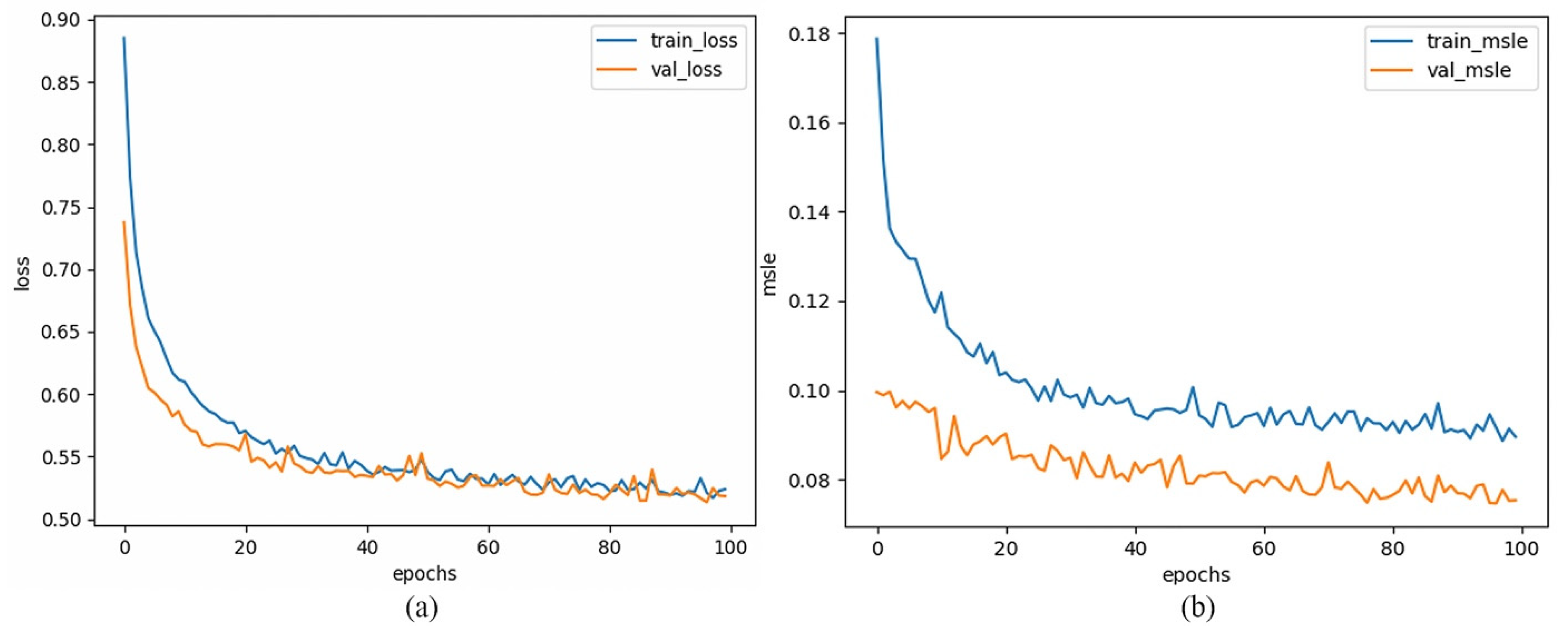
3.1. Model Performance Evaluation

The evaluation of the NO2 retrieval model is an important part of this study, using two commonly used model performance validation methods, individual validation and 10-fold cross-validation, to assess the accuracy and robustness of the model.
Firstly, individual validation was performed by dividing the dataset into the training set (80%) and the validation set (10%), with the remaining data used as the testing set (10%) to prevent overfitting of the model on the validation set. The model configuration was adjusted based on the validation data until reaching optimal performance, and finally the independent validation indicators were obtained from the model’s performance on the testing set.
The computed results show that the feature-selected 2DCNN-LSTM model exhibited high accuracy, with an R2 value of 0.87, indicating that it fits well with the target data, and the selected feature combination had a strong explanatory capacity. Furthermore, the RMSE was 6.84, indicating a small average error between the model’s validation results and the actual observations. Additionally, using all 16 channels of Himawari-8 in the model yielded an R2 of 0.74 and an RMSE of 10.93, demonstrating that the channel selection process significantly improved the performance of 2DCNN-LSTM while saving computational resources.
Subsequently, 10-fold cross-validation was performed by dividing the dataset into ten subsets, with one subset randomly chosen as the validation set and the remaining nine subsets serving as the training set. The hyperparameters were kept consistent throughout these ten validation processes, and the average performance across the ten folds was finally used as a comprehensive measurement of the model’s quality.
The 10-fold cross-validation method is commonly used over the individual validation method due to its ability to mitigate the randomness caused by a single split of the training and validation sets and fully utilize available datasets for model performance validation. This multiple splitting process helps to avoid the construction of incorrect models with inadequate generalization capabilities due to specific data splits.
To validate the accuracy of the model, the 8 h daytime (Figure 5) and the seasonal results (Figure 6A–D) were validated for further analysis. The x-axis represents the observed hourly NO2 concentrations, while the y-axis represents the near-surface concentration results obtained from the 2DCNN-LSTM model. The regression evaluation indicators, including R2, RMSE, and MAE, were used to assess the fitting effect and accuracy of the model [30]. We clustered based on the density of observation stations in various provinces in China (Figure 6E,F) to form low-density measurement regions (Tibet, Ningxia, Qinghai, and Xinjiang) and high-density measurement regions (Jiangsu, Zhejiang, Beijing, and Guangdong), and model performance was assessed. Preliminary findings suggested that differences in station density directly impacted sample size, thus affecting model estimation results. Higher-density areas with larger training sets facilitated the algorithm’s ability to identify correct patterns and trends, thereby improving accuracy as the training set size increases. The R2 of low monitoring station density regions was lower than for high density. This comparison demonstrated the direct impact of station density differences on the model’s estimation performance, but this difference was less than 0.1, indicating that it did not affect the main conclusions of the model.
The cross-validation results show that the retrieval results were well consistent with the observed values, with R2 all exceeding 0.85 and MAE within 5.70, while RMSE remained below 7.90. From morning to evening, the R2 ranged from 0.87 to 0.89, with the best performance around noon (R2 = 0.89). From spring to summer, the R2 ranged from 0.86 to 0.90, with good performance observed during the transitional seasons of spring and autumn (R2 = 0.88 and R2 = 0.90). It is noteworthy that favorable meteorological diffusion conditions (such as higher boundary layer height and high temperature) during midday lead to enhanced pollutant dispersion, as shown in the boxplot analysis in Figure 7. The low-value range of NO2 exhibited reduced dispersion compared to other concentration ranges, with the median proximity to the mean line. This quasi-normal distribution with low and unbiased dispersion diminished the retrieval error of the model. Hence, during midday, the performance of the model improved.
Additionally, the BLH generally exhibits higher levels during summer compared to autumn and winter [31]. Notably, in autumn, the correlation between NO2 vertical diffusion and BLH is more pronounced. The contribution of meteorological factors was higher in autumn than that in other seasons (as evidenced by the beta coefficient of autumn BLH was 0.27, which was higher than the 0.24 for the whole year). Therefore, the autumn 2DCNN-LSTM model performed better than the annual model, with the highest accuracy (R2 = 0.90), This was because the model covered the transition seasons when pollutant concentrations were relatively low, reducing model retrieval error and difficulty. In summer, the overall average NO2 concentration (8.58   ± 6.75 μ g / m 3 ) was lower than in other seasons, resulting in higher accuracy in predicting the target variable. However, the R2 was relatively lower, indicating a lower explanatory capability of the model for the NO2 concentrations in summer. Furthermore, the results show that around 50% of the estimated concentrations lie within the expected error. The consistency of accuracy and reliability in the daytime 8 h cross-validation and seasonal validation further confirms the stability and applicability of the model. Overall, the 2DCNN-LSTM model performed well on both hourly and seasonal scales, and was able to analyze the temporal characteristics of NO2 concentrations.
The estimation of high NO2 concentrations was influenced by multiple complex factors, including meteorological conditions and emissions sources, which may bring errors when simulating these extreme scenarios. The boxplots reflect the interquartile range, where the height of the box visually represents the data’s dispersion, with NO2 concentrations showing a right-skewed distribution and data dispersion in the high-value range. The configuration of the boxplots for high NO2 concentrations indicates that the concentration data became more dispersed with higher values, and outliers tended to be concentrated at the higher end. The model’s performance under extreme and high-concentration conditions may deviate from expectations, which can be attributed to the multifaceted influences on the estimation of high NO2 concentrations, encompassing factors such as meteorological conditions and emissions sources.

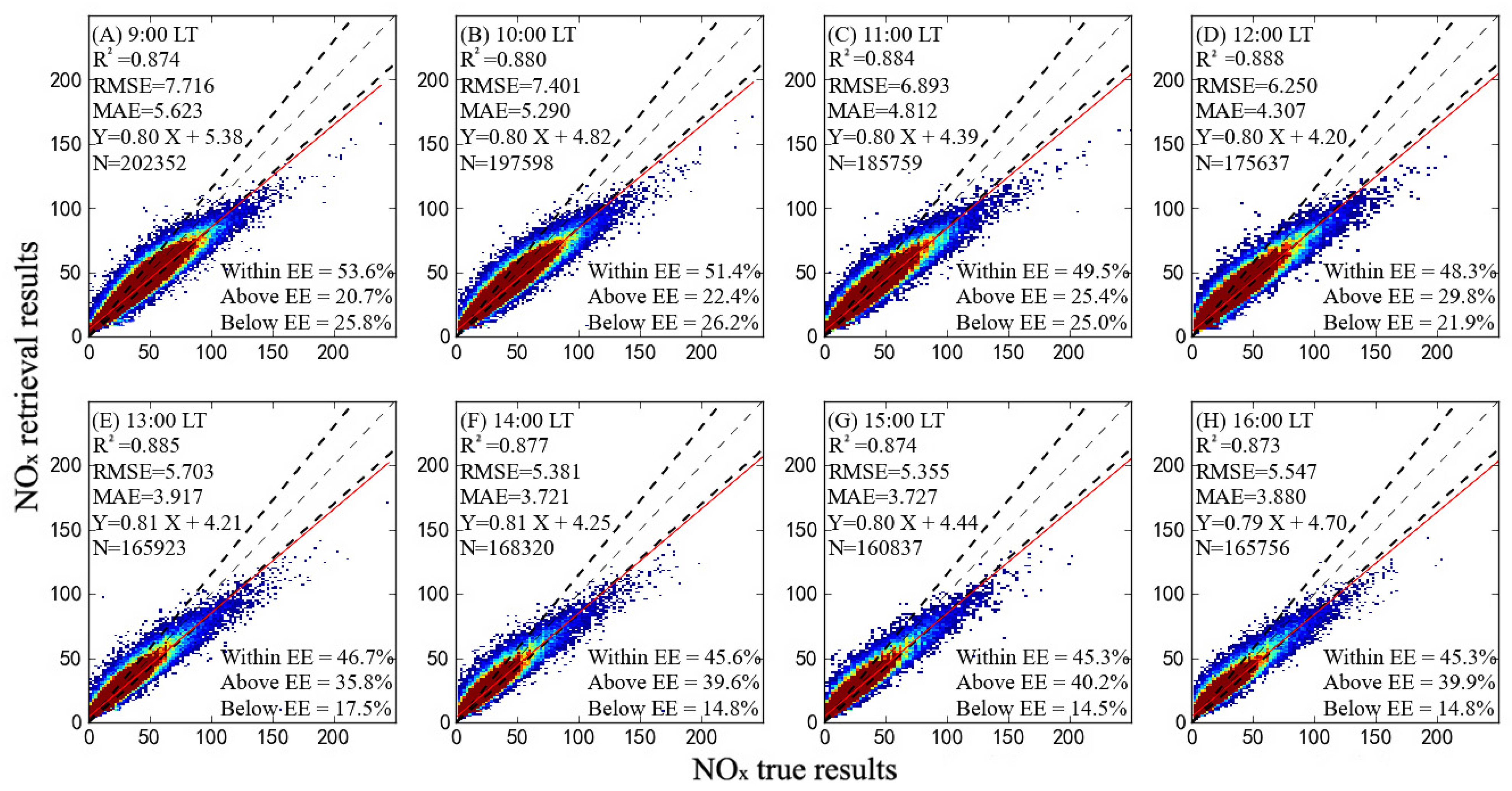
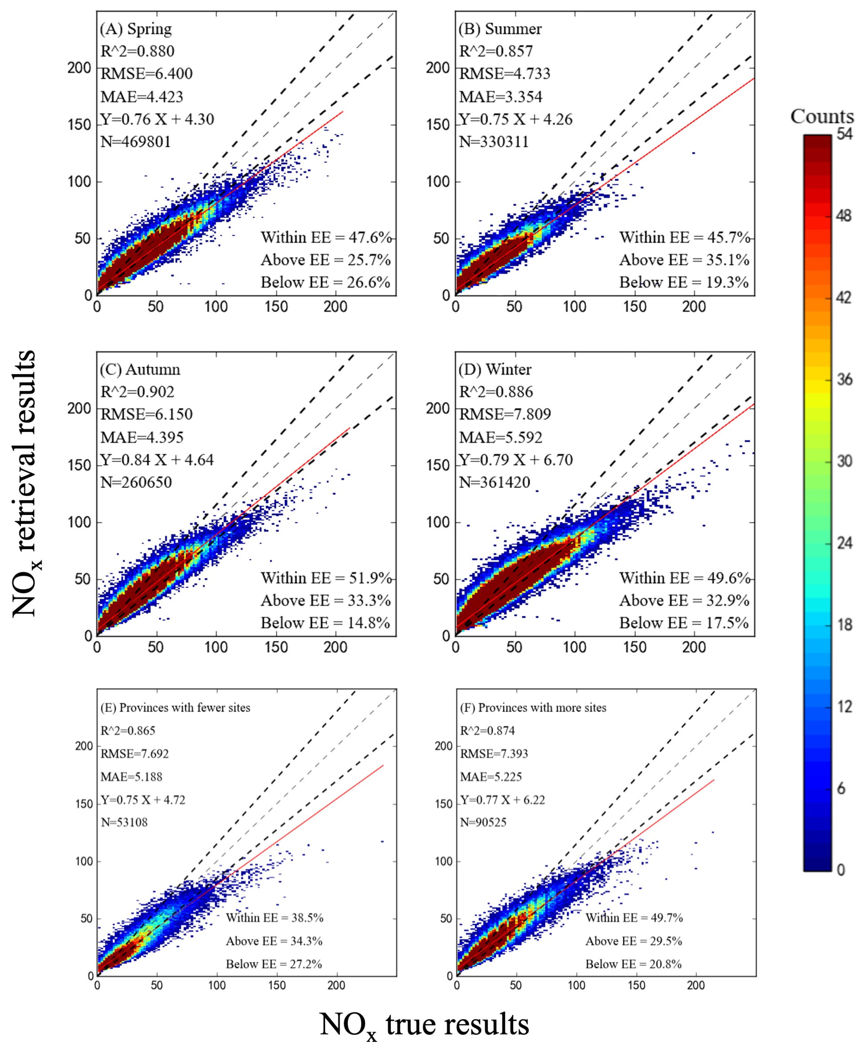
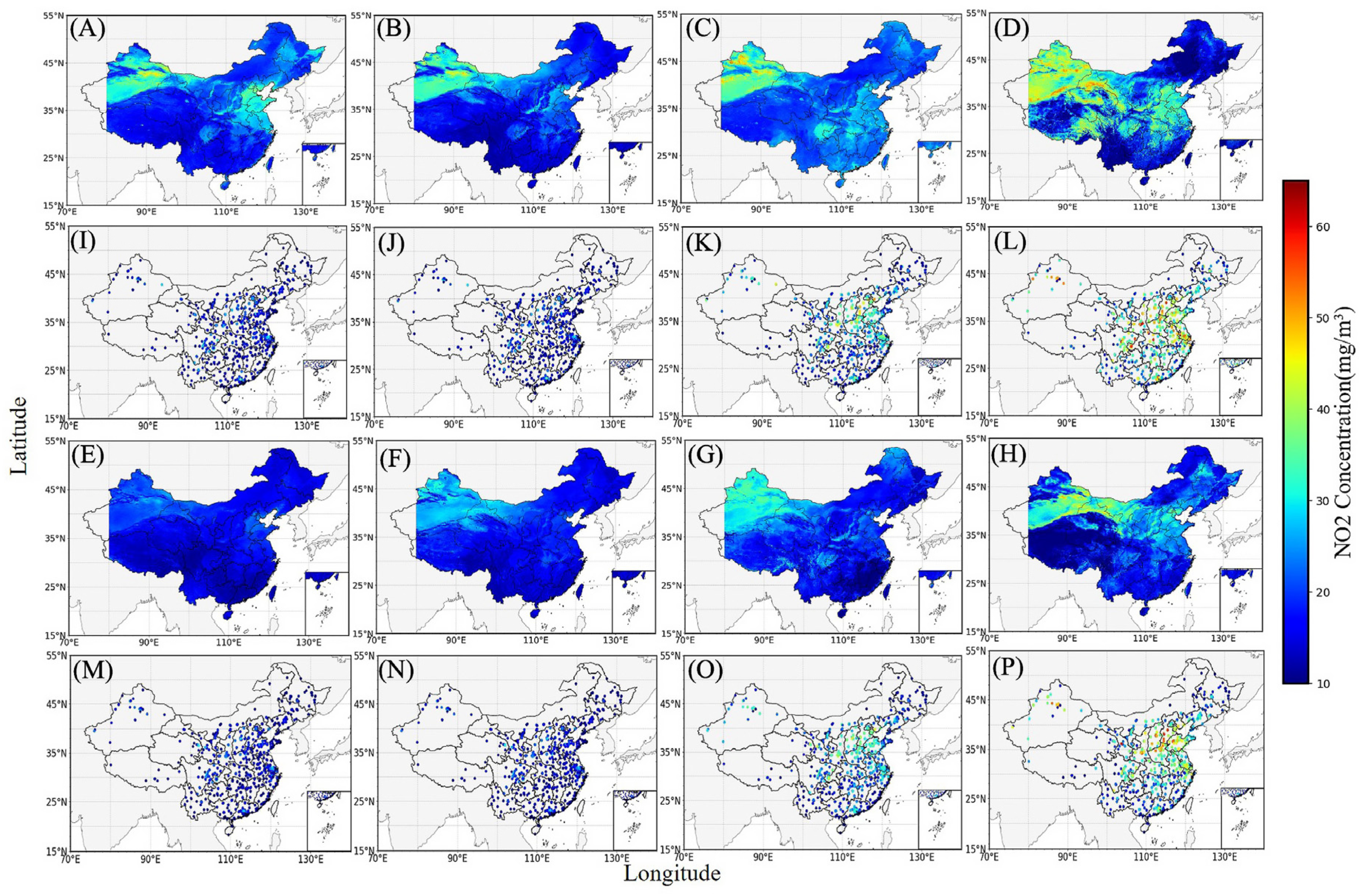
3.2. Retrieval Results

Based on the evaluation of the model, further analysis was conducted concerning the estimation results, with a particular focus on the spatial and temporal variations of NO2 distribution in different seasons from 2018 to 2019 in China.
Atmospheric NO2 is primarily derived from natural sources, while in megacity clusters and industrial regions in China, NO2 is mostly emitted from human activities such as fuel combustion, mobile sources, and stationary sources such as industrial ovens. Near-surface NO2 concentrations are generally higher in these zones due to thick population density, heavy traffic volume and high industrial emissions.
The retrieval of NO2 from 2DCNN-LSTM is in good agreement with the spatial distribution of near-surface observations. There were significant differences in the distributions of NO2 across seasons (Figure 8). Concentrations were relatively low in spring and summer, while they were rather higher in autumn and winter, especially in highly industrialized and urbanized areas. These seasonal differences were related to meteorological conditions, population density, and industrial activities. Specifically, the near-surface NO2 retrieval results based on satellite and 2DCNN-LSTM in China exhibit the following spatiotemporal and seasonal characteristics.
The seasonal characteristics of near-surface NO2 showed a low in summer and a peak in winter. The higher temperatures and increased radiation in summer promoted photochemical reactions, leading to NO2 transfer into ozone and other nitrogen-containing secondary aerosols, resulting in generally low near-surface NO2 concentrations in summer. Additionally, abundant rainfall and high humidity in summer facilitated the removal of pollutants, while the hot weather and strong atmospheric convection enhanced air mixing and the upward lifting of the atmospheric boundary layer, leading to decreased joint air stability and easy diffusion of pollutants. These factors resulted in the lowest average NO2 concentrations in summer. In winter, near-surface NO2 concentrations were highest, with a larger range of high value, mainly distributed in the Beijing-Tianjin-Hebei region, Yangtze River Delta, Pearl River Delta, Sichuan Basin, and Xinjiang. This was related to coal combustion for heating and industrial emissions in winter. Additionally, the low temperatures in winter weakened the chemical conversion of NO2 to other nitrogen compounds, and the lower surface temperature led to a decrease in the air vertical mixing and an increase in air stability, making it difficult for pollutants to diffuse. Pollution became worse when a temperature inversion occurred, resulting in the highest average near-surface NO2 concentration ( 35.11 ± 23.27   μ g / m 3 ) in winter. In the transitional seasons of spring and autumn, the average NO2 concentrations were similar, ranging from 12.20 ± 8.43   μ g / m 3 in spring to 23.49 ± 12.35   μ g / m 3 in autumn. The seasonal variation of NO2 levels was as follows: summer < spring < autumn < winter, with autumn and winter showing significantly higher levels compared to spring and summer.
From a time-series perspective, the pollutant concentrations in each season of 2019 were lower than 2018. Compared to 2018, the average NO2 concentration in 2019 decreased by 7.0%, while in spring, summer, autumn, and winter, it decreased by 7.5%, 7.1%, 2.9%, and 9.7%, respectively. In 2019, the high value zones showed a significant reduction in range and exhibited a continuous downward trend in concentrations. This trend was closely related to the ongoing environmental governance efforts [32] and the promotion of new energy vehicles in China [33]. China has been actively promoting environmental governance by implementing a series of measures to reduce pollutant emissions, such as strengthening the control of industrial and vehicular emissions, improving emission control in coal-fired electric power plants, enhancing the monitoring and early warning systems for atmospheric pollutants, and other vigorous initiatives. Furthermore, China has been promoting the popularization and use of electric vehicles, encouraging the use of clean energy transportation through providing subsidies and building charging facilities.

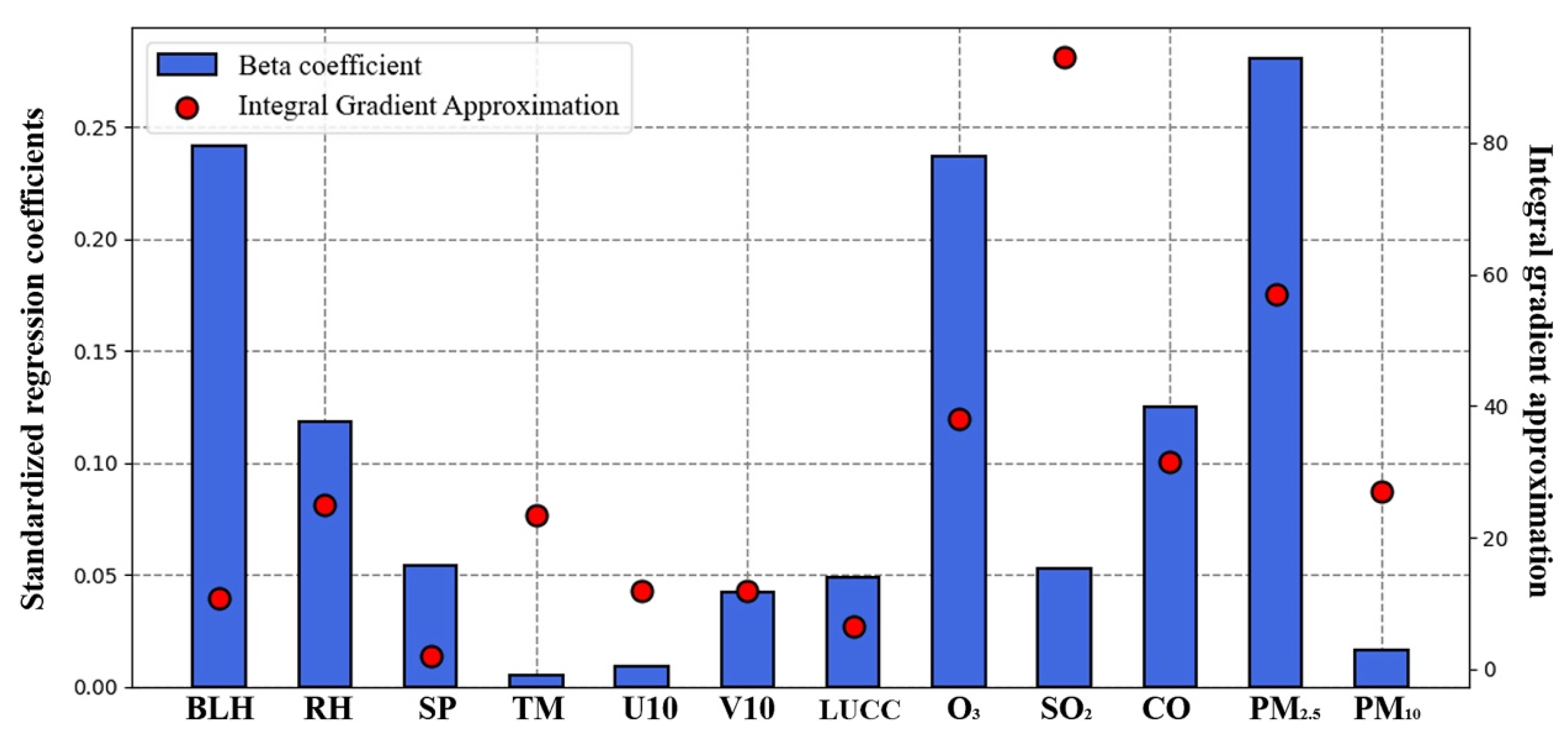
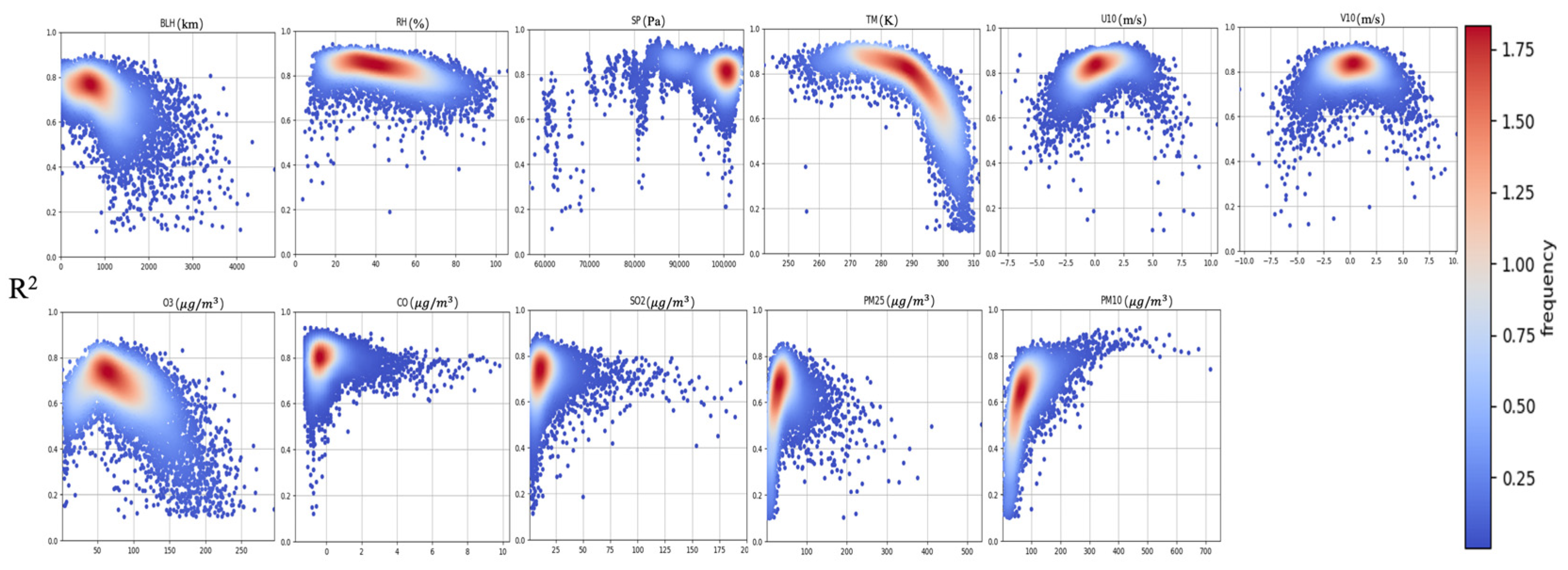
3.3. Factor Interpretability

The distribution of near-surface NO2 in China is influenced by meteorological conditions and other pollutants. Assessing factor interpretability is meaningful for interpreting the mechanisms of the black-box model and improving optimization. The following analysis examines the relationships between the considered factors, including meteorological variables (BLH, RH, SP, TM, U10, V10), other pollutant variables (O3, SO2, CO, PM2.5, PM10), as well as their contributions to the 2DCNN-LSTM model capability (Figure 9). Although other pollutant factors were not considered during the model construction, validation, and retrieval processes, exploring these influences and contributions provides guidance for coordinated pollution control among different pollutants.
The nitrate component in PM2.5 is a product of NO2 chemical transformation. Nitrate compounds in the atmosphere or adsorbed on particles can be reconverted to gaseous reactive NO2, which is an important NO2 regeneration process. According to the computed beta coefficients, PM2.5 was statistically the most influential factor on near-surface NO2, with a change of one standard deviation in PM2.5 corresponding to a change of 0.28 standard deviations in near-surface NO2. Additionally, the variation in BLH affected the air vertical mixing and the combined effects of NO2 reactions generated secondary pollutants, mainly O3, both contributing strongly to near-surface NO2 concentrations, with changes of 0.24 and 0.23 standard deviations, respectively, for a one standard deviation change in these factors.
By applying feature perturbation, the factors disrupted in order were put into the model, and the difference between the MSE of the retrieval result and the original was calculated so as to explore the contribution of one factor to the retrieval capability of the 2DCNN-LSTM model. The results show that SO2 contributed the most to the model’s retrieval capability.

4. Discussion

In order to effectively control air pollution, it is urgent to further reveal the relationship between air pollution and meteorological conditions [34]. Meanwhile, it is essential to formulate more effective policies to reduce NO2 emissions, along with strengthening the monitoring network and improving the air quality monitoring accuracy, especially in highly industrialized and urbanized zones. A study efficiently quantified the air quality response to emissions based on RFMs, obtaining that developing models to determine the response under different meteorological conditions would be beneficial for fine-scale air quality management [35]. Compared to traditional station-based monitoring, NO2 retrieval models have advantages in comparing retrieval results. With full coverage and high resolution, these models can provide more accurate and comprehensive information on NO2 distribution. Such comprehensive analysis can reveal broader pollution problems and provide more targeted data support for environmental protection and policymaking.
Moreover, the estimated distribution of NO2 showed good correspondence with highway networks, as illustrated by the distribution of national highways in China (Figure 1). For instance, the NO2 high value zone across Gansu province in each season corresponds well to G30 (Lianyungang-Horgos Highway), the NO2 high value zone along the Yellow River in Inner Mongolia exists obviously in each season, and its distribution of NO2 peaks corresponds well to G110 (Beijing-Qingtongxia Highway) in the winter. The NO2 peak zones on the east side of Tibet and the south side of Qinghai in winter correspond well with G109 (Beijing-Lhasa Highway) and G318 (Shanghai-Neramu Highway). Beijing-Tianjin-Hebei, the Yangtze River Delta, the Pearl River Delta, and the Sichuan Basin, where the transportation routes connect closely, are the obvious emission peak areas.
PAHs and BC in PM2.5 and PM10 are characterized by their composition, distribution, sources, and health risks [36], being potentially affected by regulatory actions [37]. As mentioned earlier, other pollutants and meteorological conditions can have an impact on pollutant concentrations. In order to figure out the influence of studied parameters on the model, Figure 10 displays the variation trend of the R2 concerning different feature factors, offering insight into how each parameter’s changes influence spatiotemporal patterns. The results reveal that the R2 of the estimated NO2 concentration varies with fluctuations in meteorological elements and other pollutant concentrations. In general, various factors influenced the R2 of the model. R2 increased with SP, U10, and PM10 and decreased with BLH, RH, and TM. The variation in R2 with V10 was less apparent, and other factors exhibited a trend of initially increasing to a maximum before decreasing.
The article conducted NO2 retrieval research based on satellite remote sensing technology, utilizing a fine and grid-based model to engage in an overview on the spatiotemporal distribution of pollutants in the monitoring area, and explored factor interpretability. However, there were still some research limitations. It is worth considering that the combined effects of other factors such as traffic flow and industrial emissions on NO2 concentrations have not been fully considered in this study. Meanwhile, in discussing the correspondence between NO2 retrieval results and highway networks in China, a relatively simple and intuitive graphical comparison method was used in order to more accurately measure the correspondence between the two; it is possible to construct relevant indicators to quantify the spatial and temporal correlations as well as reveal the causal relationship [38,39] of the interactions between different regions. In future studies, spatiotemporal correlations can be explored and interactions between regions can be revealed through causal analyses. With these improvements, the depth and breadth of this study can be further expanded, leading to a more comprehensive understanding of the driving mechanisms and influencing factors of NO2 concentration changes.
In addition, future research should focus on further improving and refining the model by expanding more factors, increasing research time series and validating with multi-source monitoring data. Efforts should also be made to enhance retrieval and source apportionment methods, and to strengthen model development and evaluation, so as to gain a more accurate understanding of the NO2 distribution and factor contributions. Due to the different behavior based on the seasons and regions, the clustering can be performed on different seasons and regions to train dependent 2DCNN-LSTM models with varying parameters, thus using a non-linear system with varying parameters to determine the intrinsic order certainty between the explanatory variables and the target variables in each season or districts, in order to better analyze and compare differences between seasons and geographic areas. Furthermore, further research is needed to improve related techniques and methods, enhance resolution in the retrieval process, improve data quality, and strengthen collaborative research with meteorology, environment, and other fields to promote pollution management and air quality improvement.

5. Conclusions

This study aimed to estimate near-surface hourly NO2 concentrations in China using geostationary satellite Himawari-8 data with a spatial resolution of 0.05° and to perform retrieval estimation using a parameter-optimized 2DCNN-LSTM model. The findings demonstrate that the model exhibited good fitting capacity, robustness, and had high accuracy in estimating near-surface NO2 concentrations. In terms of model performance evaluation, the channel-selected model showed further improvement compared to the original, indicating the significant impact of satellite channel selection on model performance. The 10-fold cross-validation demonstrated that the results had R-squared above 0.85 and MAE within 5.60, and RMSE within 7.90. The best validation performance was observed around noon and during the transitional seasons of spring and autumn. By analyzing the statistical methods and feature perturbation, the extent of meteorological and other pollutant factors affecting the retrieval accuracy of the 2DCNN-LSTM model was explored. The results show that BLH, O3, SO2, and PM2.5 had statistically significant contributions to the model’s retrieval capability and played important roles in estimating NO2 concentrations.
The results of this study have existing linkages with atmospheric chemistry studies and air pollution control, which are analyzed below: Firstly, the results extend the understanding of the spatial and temporal distribution of pollutants, especially in the interpretation of the changes in NO2 concentrations during urbanization. In addition, the effects of meteorological factors and other air pollutants on NO2 concentrations were analyzed in depth, which helped to reveal the sources and mechanisms of atmospheric NO2 changes. The results can provide a scientific basis for further improving air quality management and formulating corresponding policies. Finally, from the practical application point of view, this study is of great significance for monitoring and predicting air quality conditions. By establishing a spatiotemporal fine-degree NO2 detection model, the air pollution levels in different regions and seasons can be more accurately understood, thus supporting relevant departments to formulate precise pollution control measures.

Author Contributions

Conceptualization, B.C.; Methodology, R.C. and B.C.; Software, R.C.; Validation, R.C.; Formal Analysis, B.C. and R.C.; Investigation, B.C. and R.C.; Resources, B.C., R.C., J.H., Z.S., Y.W., X.Z. and L.Z.; Data Curation, B.C., R.C., Z.S., J.H., X.Z. and L.Z.; Writing—Original Draft Preparation, B.C. and R.C.; Writing—Review and Editing, B.C., R.C., J.H., Z.S. and Y.W.; Visualization, R.C.; Supervision, B.C.; Project Administration, B.C.; Funding Acquisition, B.C. All authors have read and agreed to the published version of the manuscript.

Funding

This work was supported by the National Natural Science Foundation of China (Grant number 41775021), the Gansu Provincial Science and Technology Plan (Grant number 23JRRA1038), and the Fundamental Research Funds for the Central Universities (Grant number lzujbky-2023-ey10).

Data Availability Statement

The data for the article comes from the third-party data, and the download address is given below: Global land cover data with 30 m resolution: http://data.starcloud.pcl.ac.cn/zh/resource/2, accessed on 6 April 2023; hourly near-surface pollutant concentrations were provided by the China National Environmental Monitoring Center (CNEMC) (http://www.cnemc.cn/; accessed on 6 April 2023); the Himawari-8 TOAR data were provided by the Japan Meteorological Agency (https://www.eorc.jaxa.jp/ptree/index.html; accessed on 7 April 2023); the ERA-5 data are available at https://cds.climate.copernicus.eu/cdsapp#!/dataset/reanalysis-era5-land?tab=overview; accessed on 25 April 2023.

Conflicts of Interest

The authors declare no conflict of interest.

References

  1. Sun, Q.; Hong, X.; Wold, L.E. Cardiovascular Effects of Ambient Particulate Air Pollution Exposure. Circulation 2010, 121, 2755–2765. [Google Scholar] [CrossRef] [PubMed]
  2. Vithanage, M.; Bandara, P.; Novo, L.; Kumar, A.; Ambade, B.; Gnanapragasam, N.; Ranagalage, M.; Magana-Arachchi, D. Deposition of trace metals associated with atmospheric particulate matter: Environmental fate and health risk assessment. Chemosphere 2022, 303, 135051. [Google Scholar] [CrossRef] [PubMed]
  3. Yun, G.; Yang, C.; Ge, S. Understanding Anthropogenic PM2.5 Concentrations and Their Drivers in China during 1998–2016. Int. J. Environ. Res. Public Health 2022, 20, 695. [Google Scholar] [CrossRef]
  4. Kang, H.; Zhu, B.; Zhu, C.; de Leeuw, G.; Hou, X.; Gao, J. Natural and anthropogenic contributions to long-term variations of SO2, NO2, CO, and AOD over East China. Atmos. Res. 2018, 215, 284–293. [Google Scholar] [CrossRef]
  5. He, T.; Tang, Y.; Cao, R.; Xia, N.; Li, B. Distinct urban-rural gradients of air NO2 and SO2 concentrations in response to emission reductions during 2015–2022 in Beijing, China. Environ. Pollut. 2023, 333, 122021. [Google Scholar] [CrossRef] [PubMed]
  6. Chen, B.; Hu, J.; Song, Z.; Zhou, X.; Zhao, L.; Wang, Y.; Chen, R.; Ren, Y. Exploring high-resolution near-surface CO concentrations based on Himawari-8 top-of-atmosphere radiation data: Assessing the distribution of city-level CO hotspots in China. Atmos. Environ. 2023, 312, 120021. [Google Scholar] [CrossRef]
  7. Hussain, A.J.; Sankar, T.K.; Vithanage, M.; Ambade, B.; Gautam, S. Black Carbon Emissions from Traffic Contribute Sustainability to Air Pollution in Urban Cities of India. Water Air Soil Pollut. 2023, 234, 217. [Google Scholar] [CrossRef]
  8. Ambade, B.; Sankar, T.; Sahu, L.; Dumka, U. Understanding Sources and Composition of Black Carbon and PM2.5 in Urban Environments in East India. Urban Sci. 2022, 6, 60. [Google Scholar] [CrossRef]
  9. Cheng, S.; Zhang, B.; Zhao, Y.; Peng, P.; Lu, F. Multiscale spatiotemporal variations of NOx emissions from heavy duty diesel trucks in the Beijing-Tianjin-Hebei region. Sci. Total Environ. 2022, 854, 158753. [Google Scholar] [CrossRef]
  10. Liu, J.; Chen, W. First satellite-based regional hourly NO2 estimations using a space-time ensemble learning model: A case study for Beijing-Tianjin-Hebei Region, China. Sci. Total Environ. 2022, 820, 153289. [Google Scholar] [CrossRef]
  11. Meng, K.; Xu, X.; Cheng, X.; Xu, X.; Qu, X.; Zhu, W.; Ma, C.; Yang, Y.; Zhao, Y. Spatio-temporal variations in SO2 and NO2 emissions caused by heating over the Beijing-Tianjin-Hebei Region constrained by an adaptive nudging method with OMI data. Sci. Total Environ. 2018, 642, 543–552. [Google Scholar] [CrossRef]
  12. Chen, L.; Pang, X.; Li, J.; Xing, B.; An, T.; Yuan, K.; Dai, S.; Wu, Z.; Wang, S.; Wang, Q.; et al. Vertical profiles of O3, NO2 and PM in a major fine chemical industry park in the Yangtze River Delta of China detected by a sensor package on an unmanned aerial vehicle. Sci. Total Environ. 2022, 845, 157113. [Google Scholar] [CrossRef] [PubMed]
  13. Cooper, M.J.; Martin, R.V.; Hammer, M.S.; Levelt, P.F.; Veefkind, P.; Lamsal, L.N.; Krotkov, N.A.; Brook, J.R.; McLinden, C.A. Global fine-scale changes in ambient NO2 during COVID-19 lockdowns. Nature 2022, 601, 380–387. [Google Scholar] [CrossRef]
  14. Dong, L.; Chen, B.; Huang, Y.; Song, Z.; Yang, T. Analysis on the Characteristics of Air Pollution in China during the COVID-19 Outbreak. Atmosphere 2021, 12, 205. [Google Scholar] [CrossRef]
  15. Chi, Y.; Fan, M.; Zhao, C.; Yang, Y.; Fan, H.; Yang, X.; Yang, J.; Tao, J. Machine learning-based estimation of ground-level NO2 concentrations over China. Sci. Total Environ. 2022, 807, 150721. [Google Scholar] [CrossRef]
  16. Dai, Y.; Cai, X.; Zhong, J. Chemistry, transport, emission, and shading effects on NO2 and Ox distributions within urban canyons. Environ. Pollut. 2022, 315, 120347. [Google Scholar] [CrossRef] [PubMed]
  17. Liu, J.; Cui, S.; Chen, G.; Zhang, Y.; Wang, X.; Wang, Q.; Gao, P.; Hang, J. The influence of solar natural heating and NOx-O3 photochemistry on flow and reactive pollutant exposure in 2D street canyons. Sci. Total Environ. 2021, 759, 143527. [Google Scholar] [CrossRef]
  18. Chen, Y.; Fung, J.C.H.; Yuan, D.; Chen, W.; Fung, T.; Lu, X. Development of an integrated machine-learning and data assimilation framework for NOx emission inversion. Sci. Total Environ. 2023, 871, 161951. [Google Scholar] [CrossRef] [PubMed]
  19. Guo, X.; Zhang, Z.; Cai, Z.; Wang, L.; Gu, Z.; Xu, Y.; Zhao, J. Analysis of the Spatial–Temporal Distribution Characteristics of NO2 and Their Influencing Factors in the Yangtze River Delta Based on Sentinel-5P Satellite Data. Atmosphere 2022, 13, 1923. [Google Scholar] [CrossRef]
  20. Ji, X.; Shu, L.; Chen, W.; Chen, Z.; Shang, X.; Yang, Y.; Dahlgren, R.A.; Zhang, M. Nitrate pollution source apportionment, uncertainty and sensitivity analysis across a rural-urban river network based on δ15N/δ18O-NO3 isotopes and SIAR modeling. J. Hazard. Mater. 2022, 438, 129480. [Google Scholar] [CrossRef]
  21. Liu, F.; Xing, C.; Su, P.; Luo, Y.; Zhao, T.; Xue, J.; Zhang, G.; Qin, S.; Song, Y.; Bu, N. Source analysis of the tropospheric NO2 based on MAX-DOAS measurements in northeastern China. Environ. Pollut. 2022, 306, 119424. [Google Scholar] [CrossRef]
  22. Zhang, Y.; Shi, M.; Chen, J.; Fu, S.; Wang, H. Spatiotemporal variations of NO2 and its driving factors in the coastal ports of China. Sci. Total Environ. 2023, 871, 162041. [Google Scholar] [CrossRef]
  23. Chen, B.; Wang, Y.X.; Huang, J.P.; Zhao, L.; Chen, R.M.; Song, Z.H.; Hu, J.S. Estimation of near-surface ozone concentration and analysis of main weather situation in China based on machine learning model and Himawari-8 TOAR data. Sci. Total Environ. 2023, 864, 160928. [Google Scholar] [CrossRef]
  24. Song, Z.; Chen, B.; Zhang, P.; Guan, X.; Wang, X.; Ge, J.; Hu, X.; Zhang, X.; Wang, Y. High temporal and spatial resolution PM2.5 dataset acquisition and pollution assessment based on FY-4A TOAR data and deep forest model in China. Atmos. Res. 2022, 274, 106199. [Google Scholar] [CrossRef]
  25. Yin, H.; Zhang, X.; Wang, F.; Zhang, Y.; Xia, R.; Jin, J. Rainfall-runoff modeling using LSTM-based multi-state-vector sequence-to-sequence model. J. Hydrol. 2021, 598, 126378. [Google Scholar] [CrossRef]
  26. Paoletti, M.E.; Haut, J.M.; Plaza, J.; Plaza, A. Deep learning classifiers for hyperspectral imaging: A review. ISPRS J. Photogramm. Remote Sens. 2019, 158, 279–317. [Google Scholar] [CrossRef]
  27. Ahmed, R.; Sreeram, V.; Mishra, Y.; Arif, M.D. A review and evaluation of the state-of-the-art in PV solar power forecasting: Techniques and optimization. Renew. Sustain. Energy Rev. 2020, 124, 109792. [Google Scholar] [CrossRef]
  28. Zhang, F.; Luo, L.; Li, J.; Peng, J.; Zhang, Y.; Gao, X. Ultrasonic adaptive plane wave high-resolution imaging based on convolutional neural network. NDT E Int. 2023, 138, 102891. [Google Scholar] [CrossRef]
  29. Tahmasebi, P.; Kamrava, S.; Bai, T.; Sahimi, M. Machine learning in geo- and environmental sciences: From small to large scale. Adv. Water Resour. 2020, 142, 103619. [Google Scholar] [CrossRef]
  30. Bin, C.; Song, Z.H.; Huang, J.P.; Zhang, P.; Hu, X.Q.; Zhang, X.Y.; Guan, X.D.; Ge, J.M.; Zhou, X.Z. Estimation of Atmospheric PM10 Concentration in China Using an Interpretable Deep Learning Model and Top-of-the-Atmosphere Reflectance Data From China’s New Generation Geostationary Meteorological Satellite, FY-4A. J. Geophys. Res.-Atmos. 2022, 127, e2021JD036393. [Google Scholar] [CrossRef]
  31. Guo, J.P.; Miao, Y.C.; Zhang, Y.; Liu, H.; Li, Z.Q.; Zhang, W.C.; He, J.; Lou, M.Y.; Yan, Y.; Bian, L.G.; et al. The climatology of planetary boundary layer height in China derived from radiosonde and reanalysis data. Atmos. Chem. Phys. 2016, 16, 13309–13319. [Google Scholar] [CrossRef]
  32. Hansen, M.H.; Li, H.T.; Svarverud, R. Ecological civilization: Interpreting the Chinese past, projecting the global future. Glob. Environ. Chang.-Hum. Policy Dimens. 2018, 53, 195–203. [Google Scholar] [CrossRef]
  33. Bian, X.H.; Guo, J.; Ouyang, B.; Zhang, Y.; Feng, Z.H. Prospect Analysis for the Complementary Development of Gas-Fueled and Electric Vehicles in China. 3rd Annu. Int. Conf. Sustain. Dev. (ICSD) 2017, 111, 252–258. [Google Scholar]
  34. Liu, Y.; Zhou, Y.; Lu, J. Exploring the relationship between air pollution and meteorological conditions in China under environmental governance. Sci. Rep. 2020, 10, 14518. [Google Scholar] [CrossRef] [PubMed]
  35. Cao, M.; Xing, J.; Sahu, S.K.; Duan, L.; Li, J.H. Accurate prediction of air quality response to emissions for effective control policy design. J. Environ. Sci. 2023, 123, 116–126. [Google Scholar] [CrossRef] [PubMed]
  36. Ambade, B.; Sethi, S.; Kumar, A.; Sankar, T.; Kurwadkar, S. Health Risk Assessment, Composition, and Distribution of Polycyclic Aromatic Hydrocarbons (PAHs) in Drinking Water of Southern Jharkhand, East India. Arch. Environ. Contam. Toxicol. 2021, 80, 120–133. [Google Scholar] [CrossRef] [PubMed]
  37. Ambade, B.; Sankar, T.K.; Kumar, A.; Gautam, A.S.; Gautam, S. COVID-19 lockdowns reduce the Black carbon and polycyclic aromatic hydrocarbons of the Asian atmosphere: Source apportionment and health hazard evaluation. Environ. Dev. Sustain. 2021, 23, 12252–12271. [Google Scholar] [CrossRef]
  38. Charakopoulos, A.K.; Katsouli, G.A.; Karakasidis, T.E. Dynamics and causalities of atmospheric and oceanic data identified by complex networks and Granger causality analysis. Phys. A Stat. Mech. Appl. 2018, 495, 436–453. [Google Scholar] [CrossRef]
  39. Yuan, K.; Zhu, Q.; Li, F.; Riley, W.J.; Torn, M.; Chu, H.; McNicol, G.; Chen, M.; Knox, S.; Delwiche, K.; et al. Causality guided machine learning model on wetland CH4 emissions across global wetlands. Agric. For. Meteorol. 2022, 324, 109115. [Google Scholar] [CrossRef]
Figure 1. Distribution of land cover types, air quality monitoring stations (black dots), and national highways (brown lines) in China. The black line is the China National Boundary and the provincial boundaries, with the addition of a scale (black line in the lower left corner) and a compass (upper right corner).
Remotesensing 15 04261 g001
Figure 2. Results of forward feature selection screening channels based on information entropy: entropy and information gain contained in 16 channels of Himawari-8 satellite. Left axis: information entropy; right axis: information gain. The red cross scatter indicates the information entropy value of each channel, and the dark blue diamond indicates the information gain of each channel. The seven channels covered by blue regions are subsets of the selected optimal feature channels.
Remotesensing 15 04261 g002
Figure 3. The proposed network architecture. (a) General overview of the end-to-end deep neural network model 2DCNN-LSTM. (b) Consists of three portions of CNN receiving four-dimensional tensors with spatial and temporal information as inputs, and each portion consists of a two-dimensional convolutional layer used to extract the spatial features: a Batch Normalization layer, an activation layer, and a pooling layer. (c) Two connected LSTM layers of cell states from t-1 to t: a dropout layer is inserted between the LSTMs to randomly inactivate neurons to suppress overfitting. (d) Four Dense layers that extract feature associations so that they are mapped onto the output space, with the first two Dense layers imposing a MinMaxNorm constraint and a NonNeg constraint, respectively.
Remotesensing 15 04261 g003
Figure 4. Loss falling curves: (a) Loss curves: blue line: training error; orange line: validation error. (b) Mean square logarithmic error (MSLE) curves: blue line: training mean square logarithmic error; orange line: validation mean square logarithmic error.
Remotesensing 15 04261 g004
Figure 5. The 8 h daytime 10-fold cross-validation results based on 2DCNN-LSTM (hourly cross-validation results (AH)). The black dashed line represents the expected error line, the light dashed line represents the 1:1 line, and the red solid line represents the linear regression fit line; N represents the sample size obtained each time.
Remotesensing 15 04261 g005
Figure 6. Cross-validation results based on 2DCNN-LSTM (cross-validation results for seasons from spring to summer (AD); cross-validation results with different station density regions (E,F). (E) The region of high station density consists of the provinces Jiangsu, Zhejiang, Beijing, and Guangdong. (F) The region of low station density consists of the provinces Tibet, Ningxia, Qinghai, and Xinjiang. The black dashed line represents the expected error line, the light dashed line represents the 1:1 line, and the red solid line represents the linear regression fit line; N represents the sample size obtained each time.
Remotesensing 15 04261 g006
Figure 7. The boxplots for different NO2 concentration intervals. The red x solid line is the median, the blue dashed line is the mean, and the top and bottom of the box are the upper quartile (Q3) and lower quartile (Q1) of the data, respectively.
Remotesensing 15 04261 g007
Figure 8. Spatial distribution of NO2 retrievals (AH) versus spatial distribution of stations (IP) for each season from 2018 to 2019 (unit: μ g / m 3 ) .
Remotesensing 15 04261 g008
Figure 9. Model predictability measures for the feature variables: left axis: standardized regression coefficients; right axis: approximation of the integral gradient. The blue bars indicate the corresponding beta coefficients of each factor, and red dots indicate the corresponding integral gradient values of each factor.
Remotesensing 15 04261 g009
Figure 10. Trends in the goodness of fit (R2) of feature factors.
Remotesensing 15 04261 g010
Table 1. Detailed information of the data used in this study.
VariablesImplicationTime Series LengthUnitSpatial ResolutionTemporal ResolutionData Source
NO2NO2 observation dataMarch 2018 to February 2020μg/m3siteHourlyCNEMC
TOAR1AHI blue band (0.46 μm)March 2018 to February 2020/0.05° × 0.05°HourlyJMA
TOAR2AHI green band (0.51 μm)March 2018 to February 2020/0.05° × 0.05°HourlyJMA
TOAR3AHI red band (0.64 μm)March 2018 to February 2020/0.05° × 0.05°HourlyJMA
TOAR4AHI Near-infrared band (0.86 μm)March 2018 to February 2020/0.05° × 0.05°HourlyJMA
TOAR5AHI Near-infrared band (1.5 μm)March 2018 to February 2020/0.05° × 0.05°HourlyJMA
TOAR6AHI Near-infrared band (2.3 μm)March 2018 to February 2020/0.05° × 0.05°HourlyJMA
TOAR7AHI Infrared band (3.9 μm)March 2018 to February 2020/0.05° × 0.05°HourlyJMA
TOAR8AHI Infrared band (6.2 μm)March 2018 to February 2020/0.05° × 0.05°HourlyJMA
TOAR9AHI Infrared band (6.9 μm)March 2018 to February 2020/0.05° × 0.05°HourlyJMA
TOAR10AHI Infrared band (7.3 μm)March 2018 to February 2020/0.05° × 0.05°HourlyJMA
TOAR11AHI Infrared band (8.6 μm)March 2018 to February 2020/0.05° × 0.05°HourlyJMA
TOAR12AHI Infrared band (9.6 μm)March 2018 to February 2020/0.05° × 0.05°HourlyJMA
TOAR13AHI Infrared band (10.4 μm)March 2018 to February 2020/0.05° × 0.05°HourlyJMA
TOAR14AHI Infrared band (11.2μm)March 2018 to February 2020/0.05° × 0.05°HourlyJMA
TOAR15AHI Infrared band (12.4 μm)March 2018 to February 2020/0.05° × 0.05°HourlyJMA
TOAR16AHI Infrared band (13.3 μm)March 2018 to February 2020/0.05° × 0.05°HourlyJMA
BLHBoundary layer heightMarch 2018 to February 2020m0.25° × 0.25°HourlyERA-5
TM2m temperatureMarch 2018 to February 2020K0.1° × 0.1°HourlyERA-5
RHRelative humidityMarch 2018 to February 2020%0.25° × 0.25°HourlyERA-5
U1010m u component of windMarch 2018 to February 2020m/s0.1° × 0.1°HourlyERA-5
V1010m v component of windMarch 2018 to February 2020m/s0.1° × 0.1°HourlyERA-5
SPSurface pressureMarch 2018 to February 2020Pa0.1° × 0.1°HourlyERA-5
LUCCThe type of surfaceMarch 2018 to February 2020/0.05° × 0.05°YearlyNASA
Table 2. 2DCNN-LSTM model hyperparameter settings.
Key Hyperparam EtersValue
LossMean Absolute Error
OptimizerAdam
Learning Rate0.0009
Epoch100
Batch size8
Activation functionsReLU
Regularizing functionsRegularizers.L2 (0.005)
Hidden layers30
Dropout0.05
Trainable params39,708
Disclaimer/Publisher’s Note: The statements, opinions and data contained in all publications are solely those of the individual author(s) and contributor(s) and not of MDPI and/or the editor(s). MDPI and/or the editor(s) disclaim responsibility for any injury to people or property resulting from any ideas, methods, instructions or products referred to in the content.

