Abstract
Spatial prediction of soil ammonia (NH3) plays an important role in monitoring climate warming and soil ecological health. However, traditional machine learning (ML) models do not consider optimal parameter selection and spatial autocorrelation. Here, we present an integration method (tree-structured Parzen estimator–machine learning–ordinary kriging (TPE–ML–OK)) to predict spatial variability of soil NH3 from Sentinel-2 remote sensing image and air quality data. In TPE–ML–OK, we designed the TPE search algorithm, which encourages gradient boosting decision tree (GBDT), random forest (RF), and extreme gradient boosting (XGB) models to pay more attention to the optimal hyperparameters’ high-possibility range, and then the residual ordinary kriging model is used to further improve the prediction accuracy of soil NH3 flux. We found a weak linear correlation between soil NH3 flux and environmental variables using scatter matrix correlation analysis. The optimal hyperparameters from the TPE search algorithm existed in the densest iteration region, and the TPE–XGB–OK method exhibited the highest predicted accuracy (R2 = 85.97%) for soil NH3 flux in comparison with other models. The spatial mapping results based on TPE–ML–OK methods showed that the high fluxes of soil NH3 were concentrated in the central and northeast areas, which may be influenced by rivers or soil water. The analysis result of the SHapley additive explanation (SHAP) algorithm found that the variables with the highest contribution to soil NH3 were O3, SO2, PM10, CO, and NDWI. The above results demonstrate the powerful linear–nonlinear interpretation ability between soil NH3 and environmental variables using the integration method, which can reduce the impact on agricultural nitrogen deposition and regional air quality.
1. Introduction
As an alkaline gas, ammonia (NH3) can effectively reduce the occurrence of acid rain [1,2]. NH3 can be used to synthesize fertilizers, which greatly improves agricultural productivity and meets growing food demand [3]. However, the large-scale volatilization of NH3 into the atmosphere leads to air pollution and nitrogen deposition, which leads to the eutrophication of water bodies and the destruction of biodiversity [4,5]. As an indirect source of nitrogen dioxide (N2O) emissions, NH3 has an important impact on global warming. It is estimated that the potential of carbon dioxide (CO2) to cause global warming is only about 1/265 times that of N2O in one hundred years [6,7], and global NH3 emission is projected to increase rapidly to 132 Tg by 2100 [8], with the major emission source of NH3 being agriculture. The nitrification of NH3 will lead to soil acidification and eutrophication [9]. NH3 is highly dependent on environmental variables compared to other gases due to its volatile characteristics [9,10,11]. Therefore, there is an urgent need for rapid and effective methods to predict NH3 emissions from the soil with environmental variables to provide data support for alleviating NH3 emissions or studying NH3 from soil-influencing factors.
Traditional soil NH3 measurement requires a lot of sampling work, which consumes significant manpower resources and causes cost waste. Additionally, laboratory determination requires using a concentrated sulfuric acid (H2SO4) and boric acid (H3BO3) solution. The time period for obtaining soil NH3 content is long, and it can easily cause secondary environmental pollution. Spatial prediction is an important method that can be used to realize the continuous distribution of NH3 in farmland soil in comparison with the high cost and difficulty of a soil NH3 content survey. It is essential to develop a high-performance prediction model with efficient environment variables for spatial prediction of soil NH3 flux, which is of profound significance to alleviating global warming and improving air quality.
Air quality (such as PM2.5, NO2, and SO2) has been shown to closely interact with soil ammonia. Because of the important role of NH3 in aerosol nucleation and haze [12], the gradual decrease in the formation of aerosols will lead to a significant increase in the residence time of NH3 in the atmosphere [13], while excessive NH3 stays in the aerosol phase, which may reduce the removal of the condensed phase [14]. On the contrary, the reaction of SO2 and NH3 with active radicals and NOx may also affect the formation of O3 and secondary aerosol intermediates [15,16]. Gu et al. (2022) found that the reduction in acidic precursors sulfur dioxide and nitrogen oxides in recent years has also reduced the chemical sink of NH3 in the atmosphere [13]. This is because gaseous NO2 is a reaction intermediate that reacts with NH3; NH3 has a good adsorption effect on NO2. The concentration of SO2, NO2, CO, and other precursors is significantly higher, which may impact the production of in the environment [14].
A large number of methods have been widely used in the field of soil gas flux prediction. Geostatistical interpolation is a basic method that can estimate the target of any coordinate with zero deflection and minimum variance [17,18]. For example, Roberto et al. collected 50 soil CO2 flux samples using the dynamic concentration method and interpolated the discrete points to obtain the spatial variability result of CO2 flux in the survey area based on the ordinary kriging (OK) model [19]. However, since only the spatial coordinates have no information about other auxiliary variables, the semivariogram constructed by the kriging method depends on the measured point pairs, resulting in low spatial prediction accuracy of soil gas flux [20].
With the development of artificial intelligence, the machine learning (ML) method is often used to construct the relationship between environmental variables and targets, and is applied extensively in the prediction of farmland soil gas flux [20,21]. The commonly used models include support vector machine (SVM), artificial neural network (ANN), random forest (RF), and gradient-boosted regression (GBR). For example, Abbasi et al. used the RF model with multi-source input variables (i.e., air temperature, soil organic matter, soil moisture, soil total carbon, solar radiation, etc.) to predict CO2 fluxes from the soil in the inorganic fertilizer environment in combination with field measured CO2 fluxes [22]. Morad et al. used the RF model, multivariate adaptive spline curve (MDSC), and general linear model (GLM) to predict soil NO, CO2, and nitrogen oxide fluxes under no-tillage and conventional tillage, respectively, in the case of temperature, soil moisture, and crop straw rate as environmental variables and found that the prediction results of RF model were the best [21]. Daniel et al., used quantile regression forests to predict the distribution of soil–atmosphere CH4 and CO2 fluxes in forest watersheds in different seasons by inputting DEM-derived topographic attributes [23]. The ML method is an efficient and robust substitution compared with traditional soil gas measurement methods [22,24].
However, the existing ML models suffer from two shortcomings in explaining the relationship between environmental variables and soil gases. On the one hand, the prediction performance of ML models is affected by hyperparameters. Previous studies have shown that hyperparameters can significantly affect the performance and accuracy of prediction models. Additionally, these hyperparameters also affect each other. It is difficult to capture the global optimal hyperparameters of the prediction model by using artificial trial-and-error experimentation and default hyperparameters. The automatic parameter adjustment method with high efficiency and robustness is an important auxiliary method to realize automatic ML [19]. For example, Yan et al., used a grid search (GS) algorithm to optimize and find the hyperparameters of the RF model, light gradient boosting machine (LGBM), and adaptive boosting models to adjust the parameter values so that the model performed best [25]. However, the GS algorithm is very time-consuming because it traverses all parameters in an isolated manner [26] and cannot meet the requirements of identifying global optimality [27]. Zhu et al., used an efficient Bayesian optimization method to find the optimal combination of hyperparameters of the extreme gradient boosting (XGB) model with higher prediction accuracy than GS [26]. On the other hand, the interpretation of the relationship between environmental variables and soil gas by ML is monotonous. The ML model has certain limitations on the data set and is suitable for nonlinear data sets [21], ignoring the spatial autocorrelation between adjacent observation data [28].
A new prediction model, the integration kriging model, has been proven to be more accurate in predicting soil properties in many current studies [29,30,31,32,33,34,35]. For example, Guo et al. found that the integration method has advantages in predicting the spatial variability of soil organic matter in the case of comparing the methods of RF, stepwise linear regression (SLR), and the combination of RF and residual kriging by inputting topographic attributes, such as geological units, climate factors, and vegetation indices [28]. Based on 73 years of NO2 observation data from 14 monitoring stations, Chen et al. predicted the spatial–temporal characteristics of NO2 concentrations in Taiwan using the NO2 data interpolated kriging method and the land use regression model with local non-traditional geographical predictors [36].
However, whether the integration of the TPE-based ML model and geostatistical model can significantly improve the spatial prediction accuracy and explain the relationship between environmental variables and soil NH3 flux is still unclear (i.e., nonlinear and linear coupling characteristics). Therefore, to overcome the limitations of the hyperparameter adjustment and spatial autocorrelation neglect of ML modeling, the objective of this study is to demonstrate the increased predicted model performance using TPE–ML–OK-based models with Sentinel-2 remote sensing image and air quality data, which involves establishing ML models, determining the optimal hyperparameters using the TPE algorithm, building a residual ordinary kriging model, and revealing the relationships between key variables and soil NH3 flux via explainable analysis. The environment variables (i.e., Sentinel-2 remote sensing image and air quality data) related to soil NH3 were collected first. Then, the tree-structured Parzen estimator (TPE) search was applied to find the optimal hyperparameters of the gradient boosting decision tree (GBDT), random forest (RF), and extreme gradient boosting (XGB) models, and the residual ordinary kriging model was used to further predict and mapping the soil NH3 flux. Finally, the relationships between environmental variables and soil NH3 were evaluated using the SHapley additive explanation (SHAP) method.
2. Materials and Methods
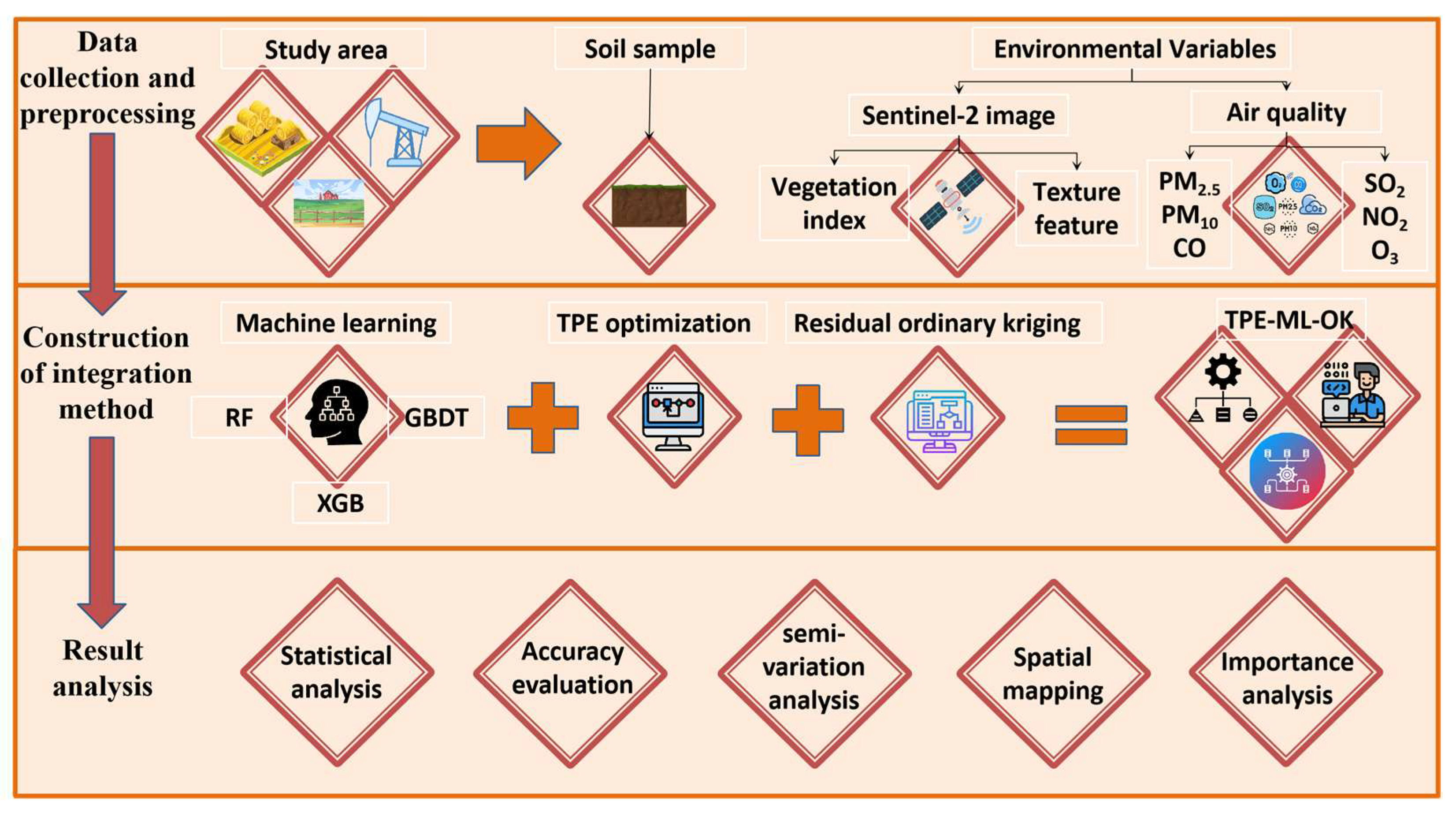
Figure 1 shows the flowchart in this study and includes three phases: (i) collection and preprocessing of sampling and environmental variable data (vegetation index and texture features from Sentinel-2 L2A image, interpolation analysis of air quality stations data, and soil NH3 sampling); (ii) construction of integration method (machine learning model, TPE hyperparameter optimization, and residual ordinary kriging); and (iii) accuracy evaluation of prediction results, soil mapping using TPE–ML–OK models, and importance analysis of environmental variable using the SHAP method.
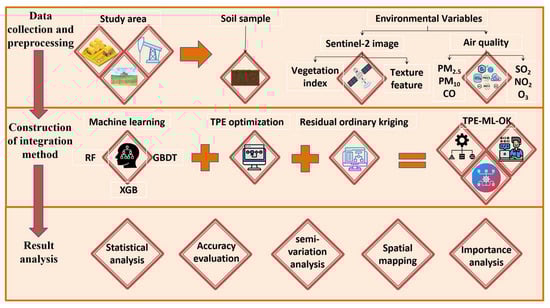
Figure 1.
The method workflow of this study.
2.1. Overview of Study Area
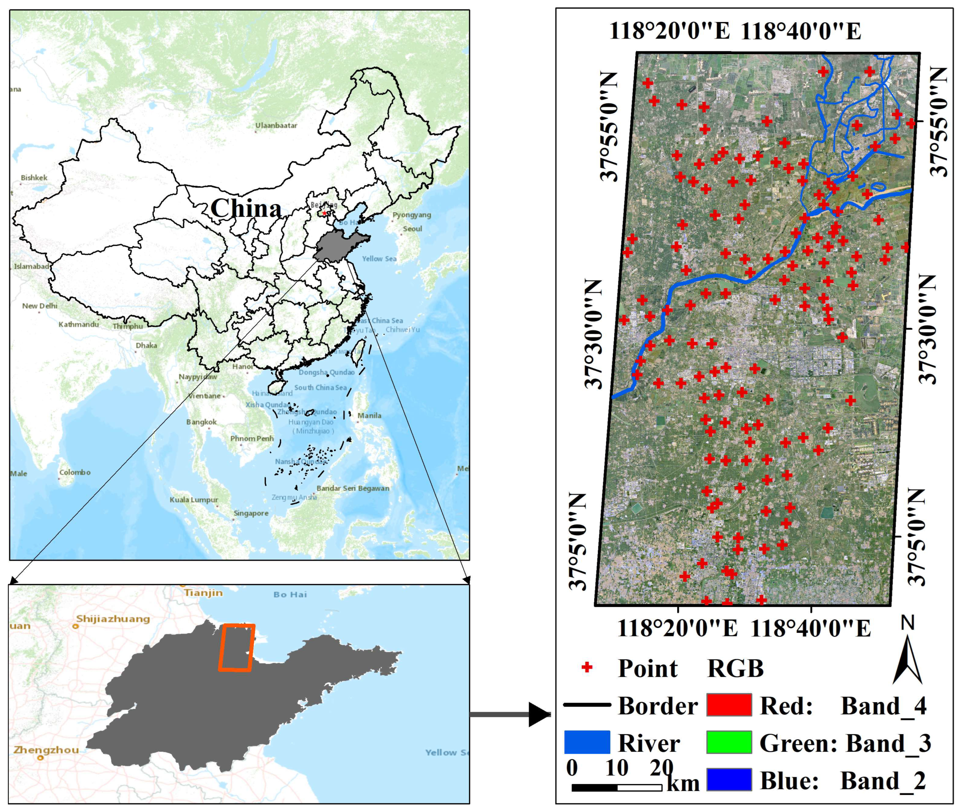
The study area is situated in the Yellow River Delta (YRD), East China (36°55′–38°10′N, 118°07′–119°10′E). It has a temperate continental monsoon climate, and the terrain inclines from southwest to northeast along the Yellow River (Figure 2). Soil types are divided into five categories: cinnamon soil, Shajiang black soil, fluvo-aquic soil, saline soil, and paddy soil. Based on the statistical yearbook of Dongying in 2020, the average temperature in the study area is 14.1 °C, the annual precipitation is 665.3 mm, and the annual sunshine hours are 2998.5 h. The study area mainly contains oil, natural gas, oil shale, and many other mineral resources, which is the main production area of the Shengli Oilfield. However, the soil pollution caused by oilfield development in this area indirectly affects the survival rate of soil microorganisms and, thus, the absorption, transformation, and utilization of NH3 by some soil microorganisms, which changes the NH3 content in the soil. Spatial prediction of soil NH3 is of great significance in improving microclimate change, air pollution, and nitrogen loss from farmland in the study area.

Figure 2.
The study area location and sampling points of NH3 in farmland soil.
2.2. Soil Sample Collection and Analysis
In the farmlands of the study area, 134 sampling points were uniformly and randomly arranged from 22 September 2022 to 29 September 2022. The NH3 volatilization was measured per day at 8:00–10:00 a.m. and 3:00–5:00 p.m. The concentration of NH3 was determined using the continuous airflow enclosure method, and a cylindrical plexiglass chamber (20 cm in diameter and 30 cm in height) was installed in the soil of each sample plot. We inserted the air chamber into the soil of 5 cm and connected the air in the glass chamber from the air outlet to the pump-suction gas-phase speedometer (FZ2800-2, Guangzhou, China) through the pipeline. The measurement interval of each sample point was 10 min, the measurement was carried out in three parallels, and the initial and final NH3 content (unit ppm) was recorded on the spot. The initial NH3 content was converted into emission flux (unit: kg N ha−1 d−1) according to Equation (1) [37,38].
AE represents the volatilization flux of NH3 in farmland soil, c represents the content of soil NH3 (m mol mol−1) from the pump-suction gas-phase speedometer, v represents the air velocity (0.25 L min−1), 14 represents the molar mass of NH3 (g mol−1), 1440 represents the conversion from min−1 to d−1 (1 d 1440 min), 106 represents the conversion from m−2 to ha−1, 10−9 represents the conversion from mg N into kg N, mv represents the molar volume of the NH3, and 0.0177 is the covered area of the air chamber (m2).
2.3. Environmental Variables
2.3.1. Remote Sensing Data
Based on the Sentinel-2 L2A remote sensing image (23 September 2022), the remote sensing index was calculated and obtained. The data comes from the European Space Agency (https://scihub.copernicus.eu/, accessed on 12 November 2022). The L2A image data were preprocessed (i.e., atmospheric correction), and four vegetation index factors were calculated using band 2, band 3, band 4, band 5, band 6, and band 8, including visible atmospheric resistant index (VARI), soil-adjusted vegetation index (SAVIred), normalized difference water index (NDWI), and plant senescence reflectance index (PSRI) (Table 1); the resolution of all vegetation variables was 10 m × 10 m.

Table 1.
Indexes derived from Sentinel-2 L2A image.
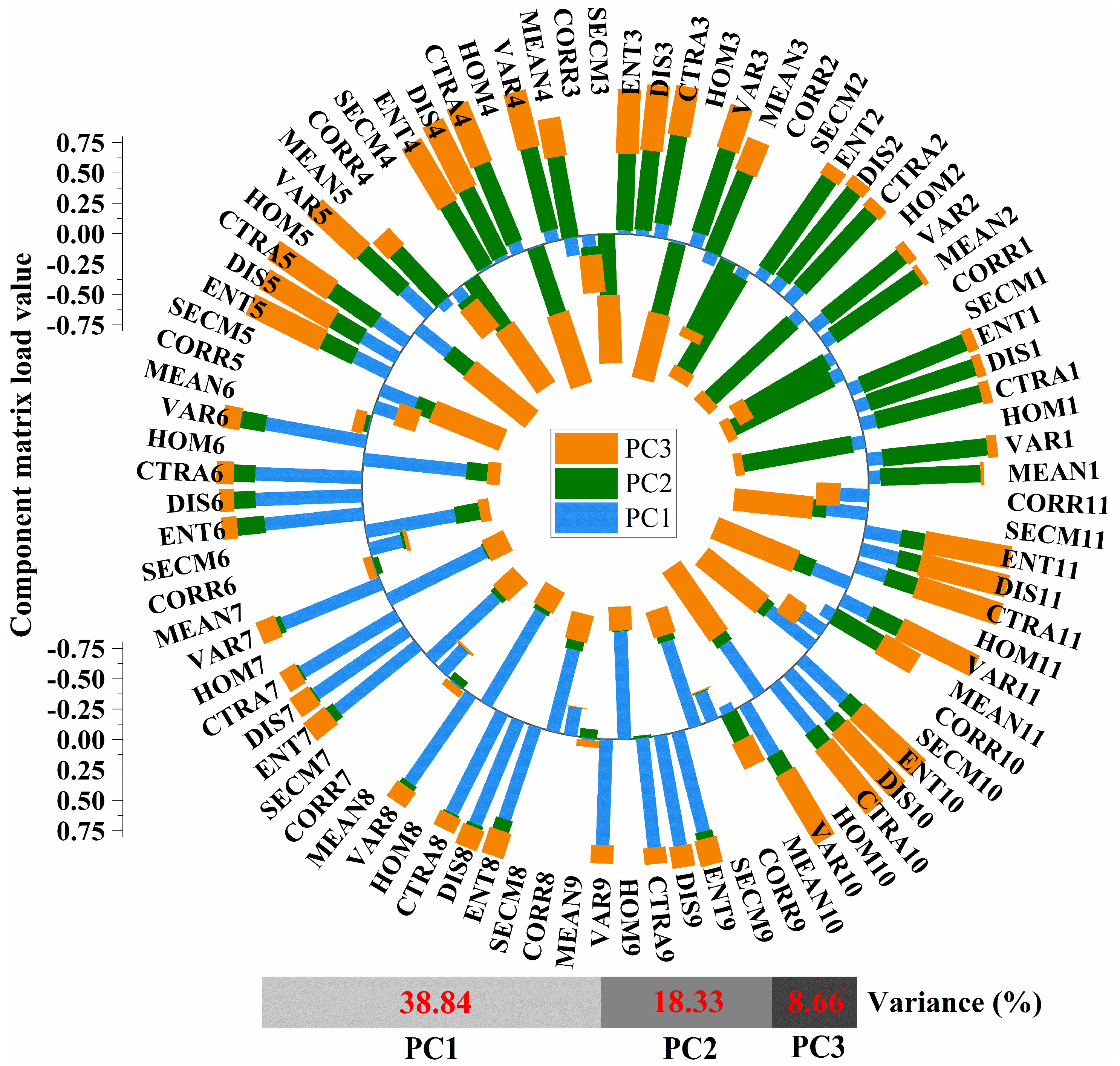
Texture features can reflect additional information, such as hue changes and attributes of remote sensing images, and have been widely used in the extraction or classification of ground object information [43,44,45]. For example, many studies have used the GLCM method to calculate the relative frequency between the pixel brightness values of remote sensing images to obtain spatial information gain, which effectively improves the interpretation and classification accuracy of ground objects [46,47,48]. Based on the 11 bands of the preprocessed Sentinel-2 L2A image, the texture features were also calculated and analyzed using filter/co-occurrence measures in ENVI 5.3 software. A total of 88 texture features were obtained, including eight transformations: entropy (ENT), correlation (CORR), mean (MEAN), homogeneity (HOM), contrast (CTRA), dissimilarity (DIS), angular second moment (SECM), and variance (VAR). In order to simplify the variable dimension, the first three principal components were obtained using principal component analysis (PCA) in ENVI 5.3 software, and the total variance contribution rate that can be explained is 65.83%. The features with high load values of PC1, PC2, and PC3 were mainly concentrated in band 6–band 9; band 1–band 4; and band 5, band 10, and band 11 after texture transformation (Figure 3). These principal components (PC1–PC3) representing image texture features can reflect soil physical information such as spatial information (i.e., pattern, shape, size, etc.), geometric morphology, texture, and coverage on the soil surface, and have important implications for the basic soil conditions of NH3 emissions.
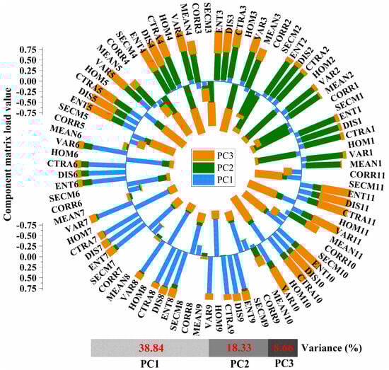
Figure 3.
Component matrix load value of principal component analysis based on Sentinel-2 L2A image.
2.3.2. Air Quality
The air quality in the study area indirectly interfered with soil microbial interaction, affecting soil NH3 emissions. In order to be consistent with the sampling time of soil NH3, the selected time of air quality data was the monthly average of September 2022. Six air quality pollutants (CO, NO2, O3, PM2.5, PM10, and SO2) were obtained as environmental variables for spatial prediction of NH3. The data were obtained from the real-time air quality release system (http://218.58.213.53:8081/dyfb_air/fb_web/dongying.html, accessed on 10 November 2022) of Dongying Environmental Protection Bureau, including 40 air quality monitoring stations. The air quality data of all stations were processed using interpolation analysis with a resolution of 10 m × 10 m in ArcGIS 10.7 software.
2.4. Machine Learning Model
2.4.1. Random Forest
Random forest (RF) is a tutorial integration algorithm with a decision tree as a base estimator [49]. In the modeling process of RF, different subsets are randomly sampled from the provided dataset and then used to build multiple decision trees. According to bagging rules, the results of several decision trees were synthesized to predict soil NH3 fluxes, that is, the average values of the results output by several base estimators. The learning ability of the RF model is strong, and it can overcome the over-fitting problem caused by a highly dimensional variable input. The RF model has been widely used in soil, ecology, and other fields [50,51,52]. The core hyperparameters of the RF model that need to be optimized are shown in Table 2. For example, max_depth and max_features have a significant impact on the prediction accuracy and splitting depth of the basic estimator.
Table 2.
Information description of core hyperparameters of RF model.
2.4.2. GBDT
Gradient boosting decision tree (GBDT) is one of the ensemble ML models that uses classification and regression tree (CART) as the basic model [53]. Different from the bagging rule of the RF model, the GBDT model meets the basic process of the boosting rule, calculates the loss function based on the results of the previous base estimator, and uses the loss function to affect the next base estimator (Equation (2)) [53].
and represent the n-th (n ≥ 1) and n − 1 weak learners, respectively. represents a new learner based on the residual of the n − 1 weak learner. The current i-th learner in the GBDT model is affected by all previously trained weak learners [49,54,55] and finally integrated multiple base estimators and output soil NH3 prediction values. Because GBDT is optimized in the base estimator, loss function, fitting residual, and random sampling, it has a stronger learning ability than most boosting algorithms. GBDT is one of the most stable machine learning algorithms in actual scenarios. The core hyperparameters and information of the GBDT model are shown in Table 3.
Table 3.
Information description of core hyperparameters of GBDT model.
2.4.3. XGB
The eXtreme gradient boosting (XGB) is a new machine-learning model proposed by Chen et al. in 2016. It has been optimized based on the GBDT algorithm, making XGB have better results in dealing with regression and classification problems [51,52]. As an advanced boosting algorithm, XGB builds the next weak learner based on the results of the previous weak learner in each iteration [53]. The advantage of the XGB algorithm is that the objective function with a regular term controls overfitting [54]. In addition, similar to the RF model, XGB also supports column sampling, which extracts some data for training during the iteration process so as to control overfitting by reducing the amount of calculation. Compared with the first-order Taylor expansion of GBDT, XGB adopts the second-order Taylor expansion, which can approximate the real loss function more accurately. Equation (3) shows the objective function () [51].
where and represent the i-th measured value and the predicted value at step t, respectively, L represents the loss function, Ω represents the regular term, and represent the i-th input variables and the k-th tree, respectively, and and represent the first and second derivatives of the L, respectively. Then, the final objective function (Equation (4)) at the j-th leaf is as follows:
where T represents the total leaf nodes of the XGB model, and represent the scores on the j-th leaf and complexity of leaf nodes, respectively, and is a compromise parameter that scales the penalty. The core hyperparameters and information of the XGB model are shown in Table 4.
Table 4.
Information description of core hyperparameters of XGB model.
2.4.4. TPE Search Algorithm
Not only is the internal structure of the above prediction model complex, but many hyperparameters also need to be adjusted. Moreover, the hyperparameters have a great influence on the prediction performance of the model [55,56]. Hyperparameters usually refer to the parameters shared between different modules, functions, classes, or objects in the model. These parameters can be used by multiple components to achieve data transfer, interaction, and sharing of information. The traditional manual adjustment will take a lot of time and cost, and the effect is not good. Studies have shown that compared with the GS algorithm, the Bayesian optimization (BO) algorithm cannot easily plunge the local optimum and is more efficient. Bayesian optimization is considered the most advanced superparameter optimization framework at present and is widely used in various fields of AutoML [57]. It uses the frequency of the minimum value to judge. The frequency reflects the probability of the minimum value to some extent. The higher the frequency, the greater the probability that the function has a minimum value. Tree-structured Parzen estimator (TPE) is one of the most advanced BO algorithms based on tree-structured Parzen density estimation. First, the TPE algorithm defines two probability density functions (Equations (5) and (6)) based on (i.e., the value at the quantile r in the y-set).
Then, the TPE optimization algorithm selects EI (expected improvement) as the evaluation criterion (Equation (7)):
Finally, we can obtain Equation (8):
In Equation (8), we can see a direct correlation between the value of EI and the value of . In order to improve EI, we make the probability of as large as possible and the probability of as small as possible so as to select the most suitable x value. In each iteration, the algorithm returns with the maximum EI value, and the returned will participate in the next iteration so as to repeatedly find the best hyperparameter combination of the soil NH3 prediction model. In this study, packages (i.e., xgboost, sklearn.model_selection, sklearn.ensemble, hyperopt, etc.) are imported into the Python 3.9 programming environment to build the above algorithms (i.e., RF, GBDT, XGB, and TPE).
2.5. The Integration Method
The integration method was used to further improve the prediction accuracy of soil NH3 flux. First, the residual value between the true value of soil NH3 and the predicted value of the TPE-optimized ML method (i.e., TPE-GBDT, TPE-RF, and TPE-XGB) was calculated (Equation (9)).
Then, the ordinary kriging (OK) interpolation algorithm was used in ArcGIS 10.7 software to obtain the residual spatial continuity distribution of the TPE-optimized machine learning model. The formula of the OK model (Equations (10) and (11)) is as follows [58]:
where represents the experimental semivariogram in the kriging interpolation process, represents the number of sampling points separated by h (where h is the lag distance between and , and is the optimal weight. ArcGIS 10.7 software was used to realize the spatial interpolation calculation of the OK model. Finally, the spatial prediction results of soil NH3 flux in the hybrid geostatistical model were obtained by adding the spatial prediction value of the TPE-optimized machine learning model to the residual kriging value (Equation (12)) [59].
where includes the comprehensive prediction results of tree-structured Parzen estimator–random forest–ordinary kriging (TPE–RF–OK), tree-structured Parzen estimator–gradient boosting decision tree–ordinary kriging (TPE–GBDT–OK), and tree-structured Parzen estimator–extreme gradient boosting–ordinary kriging (TPE–XGB–OK), representing the optimal spatial estimation of soil NH3 flux.
2.6. Verification
In this study, the datasets were randomly divided into 70% for the training set and 30% for the test set to build a prediction method. For accuracy evaluation, root mean square error (RMSE) (Equation (13)) and coefficient of determination (R2) (Equation (14)) were used. and are, respectively, the real value of soil NH3 flux and the prediction value of the super parameter optimization model, and and are, respectively, the average of the real value of soil NH3 at all sample points and the average of the estimated value of the model.
Because the ensemble learning models, deep learning models, and other models are extremely complex, abstract, and difficult to understand, the importance score of each environmental variable was output and visualized using the SHapley additive explanation (SHAP) analysis so that we can determine which environmental variables play a leading role in affecting soil NH3 flux. As a unified interpretation framework, SHAP can calculate the importance score of each feature in the data so as to explain the model. In this study, the SHAP package was imported into the Python 3.9 programming environment to explain the predicted method and visualize the importance of different environment variables.
3. Results and Analysis
3.1. Statistical Analysis
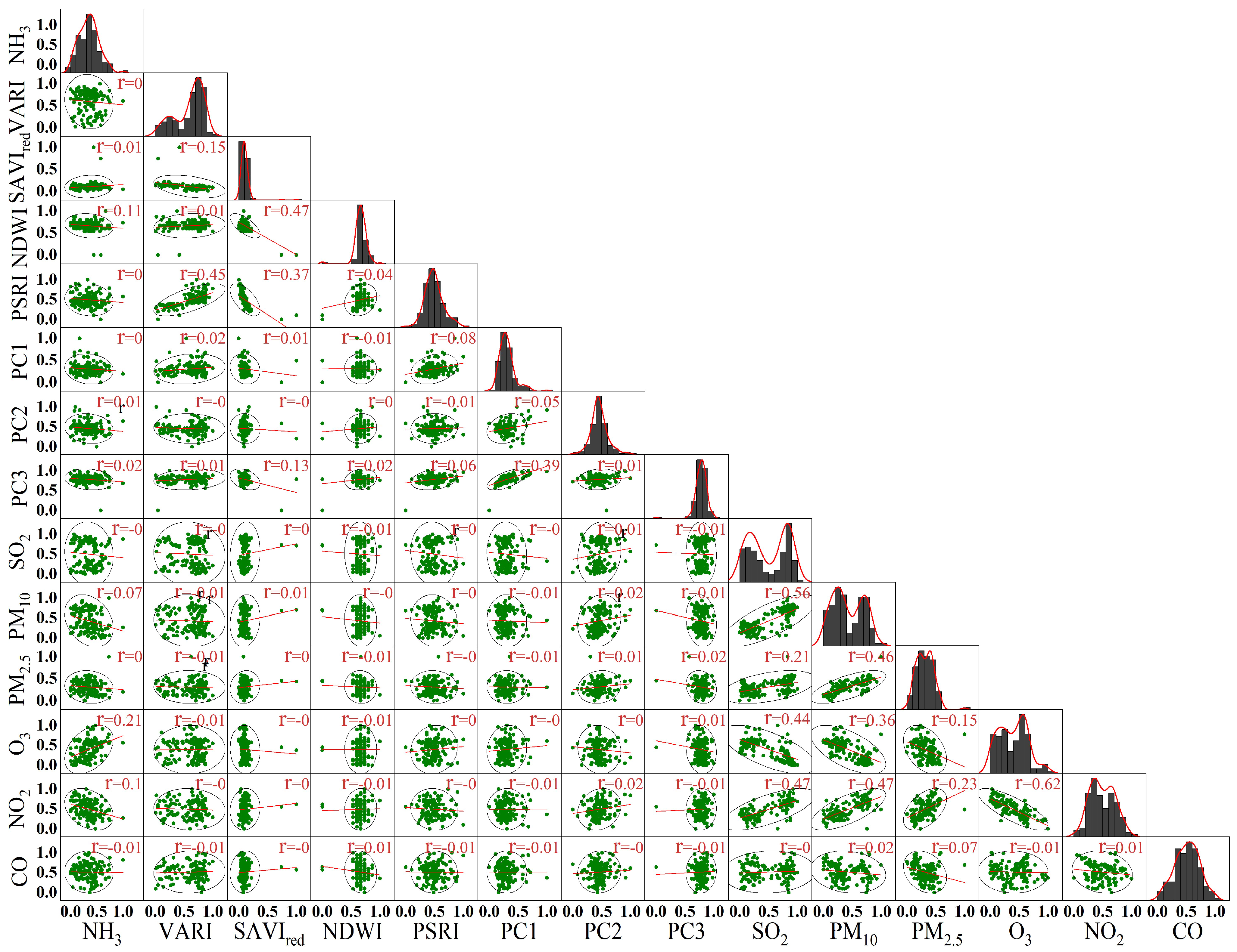
Figure 4 shows the normalized numerical distribution of NH3 flux in soil and auxiliary variables. The soil NH3 fluxes are concentrated in the median area, and the data structure is normally distributed. PSRI, PC1, and PC2 also showed significant normal distribution. However, the values of other variables showed skewed or bimodal distribution. There were significantly nonlinear characteristics among different environmental variables. The linear correlation between similar variables was strong, the positive linear correlation between vegetation index factors (i.e., SAVIred and NDWI, VARI and PSRI, and SAVIred and PSRI) was high (r > 0.2), the negative linear correlation between soil texture factors (PC3 and PC1) was strong (r = 0.39), and there was a high correlation between air quality variables. Obviously, there was a positive linear correlation between soil NH3 flux and O3 (r = 0.21) and a weak linear correlation with other variables. The above correlation analysis results show complex fitting characteristics between soil NH3 flux and environmental variables.
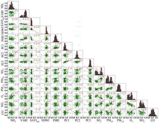
Figure 4.
Matrix scatter plot between soil NH3 flux and environmental variables. The r is the value of Pearson correlation value.
3.2. Spatial Prediction of Soil NH3 Using TPE–ML–OK Method
3.2.1. Evaluation of Hyperparameter Optimization Process
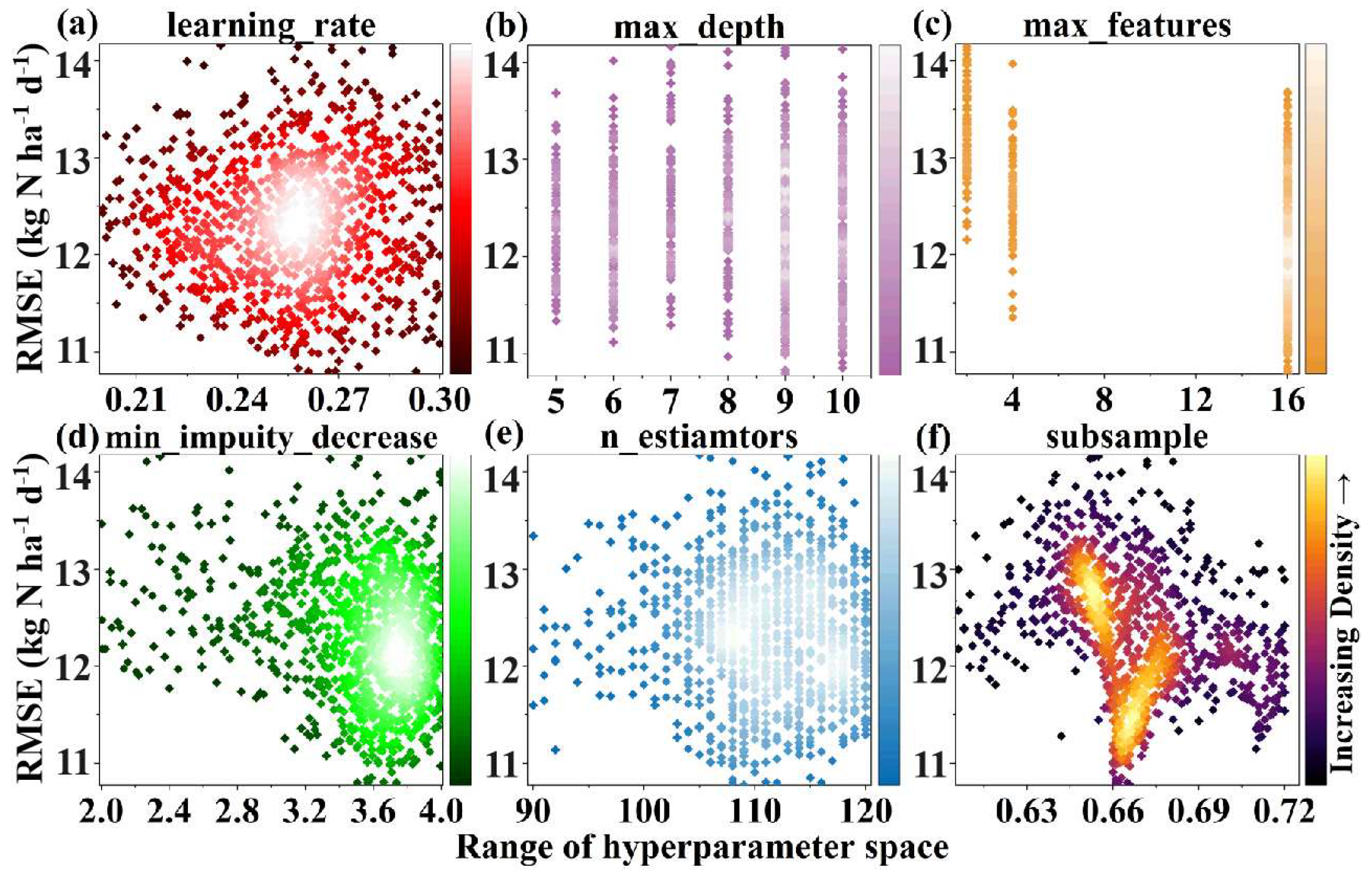
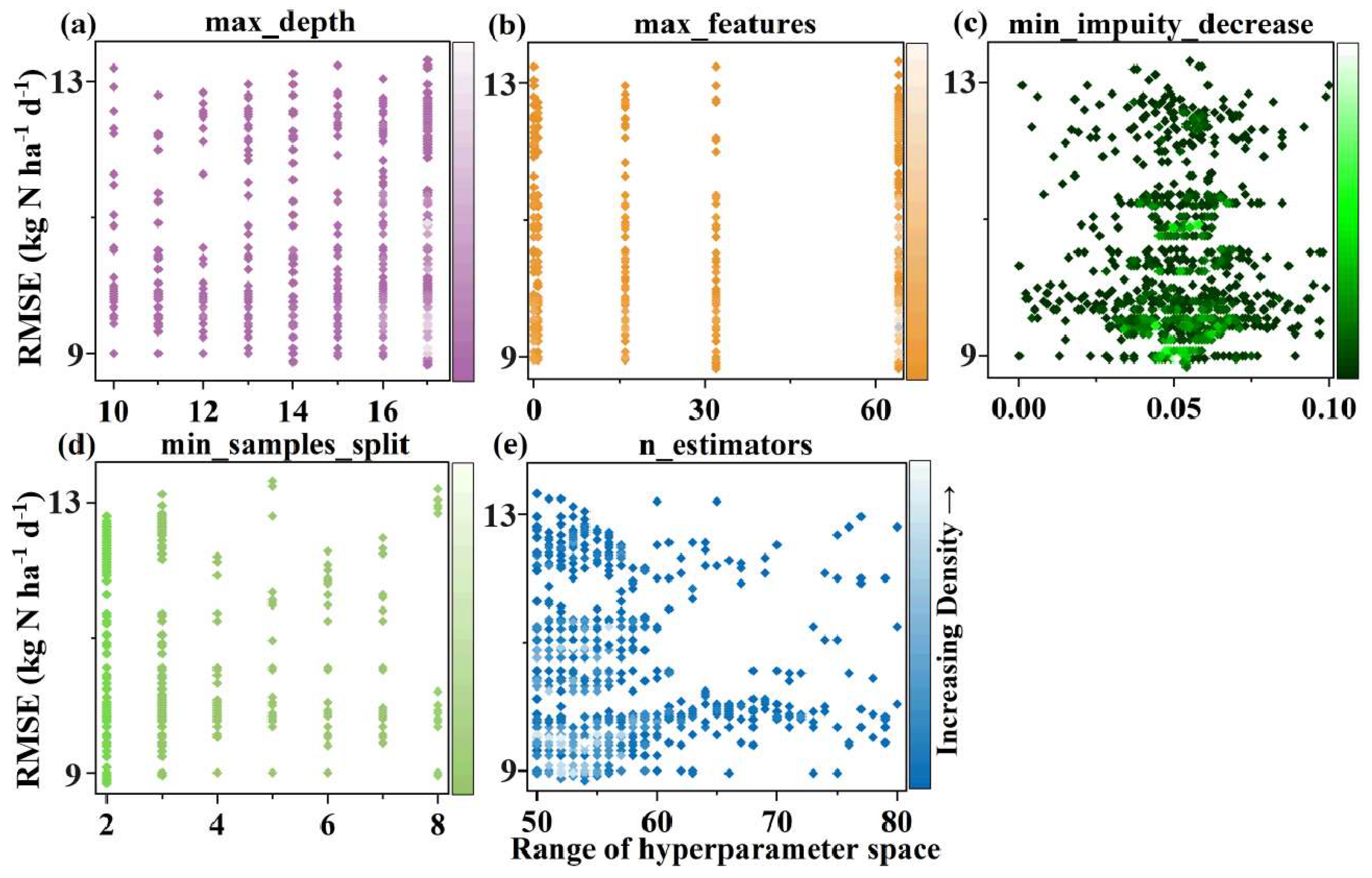
Figure 5, Figure 6 and Figure 7 show the sampling point iteration trend of GBDT, RF, and XGB models in the TPE optimization process, respectively. Obviously, the sampling points in the TPE optimization process have an aggregation trend, and there is a region with the densest distribution of sampling points in each hyperparameter iteration process. For example, some hyperparameters (min_impuity_decrease of the GBDT model and min_child_weight of the XGB model) increase with the increase in the value, and the distribution of sampling points change from sparse to dense. Other hyperparameters (n_estimators of the RF model and colsample_bynode of the XGB model) show the trend of sampling points from dense to sparse (that is, it is difficult to reach the optimal value, even if the hyperparameter value is increased). These sampling-intensive areas are significantly different from the sparse sampling areas, and the optimal parameters often appear near the sampling-intensive areas. The lowest RMSE values obtained by the RF, GBDT, and XGB models in the TPE optimization process are relatively close, which are 11.96 kg N ha−1 d−1, 11.77 kg N ha−1 d−1, and 11.70 kg N ha−1 d−1, respectively, indicating that the TPE algorithm has strong generalization in the hyperparameter optimization of different models. TPE always selects the next set of sampling points according to the results of previous sampling points [60]. After multiple iterations, the probability that the optimal hyperparameters appear in the dense sampling area is much higher than in the sparse area.
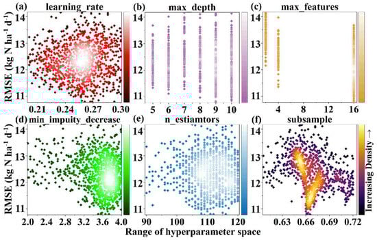
Figure 5.
TPE optimization process of GBDT model hyperparameters.

Figure 6.
TPE optimization process of RF model hyperparameters.
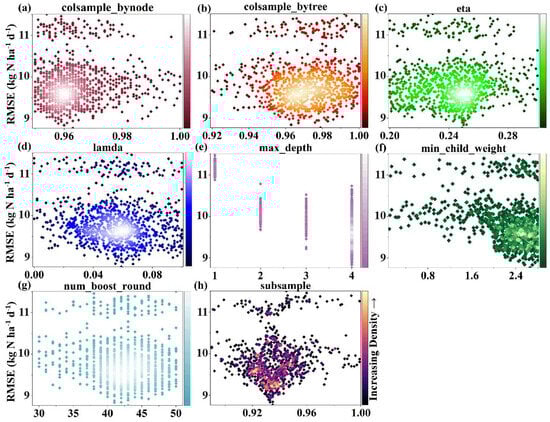
Figure 7.
TPE optimization process of XGB model hyperparameters.
3.2.2. Prediction Accuracy of TPE–ML Model for Soil NH3
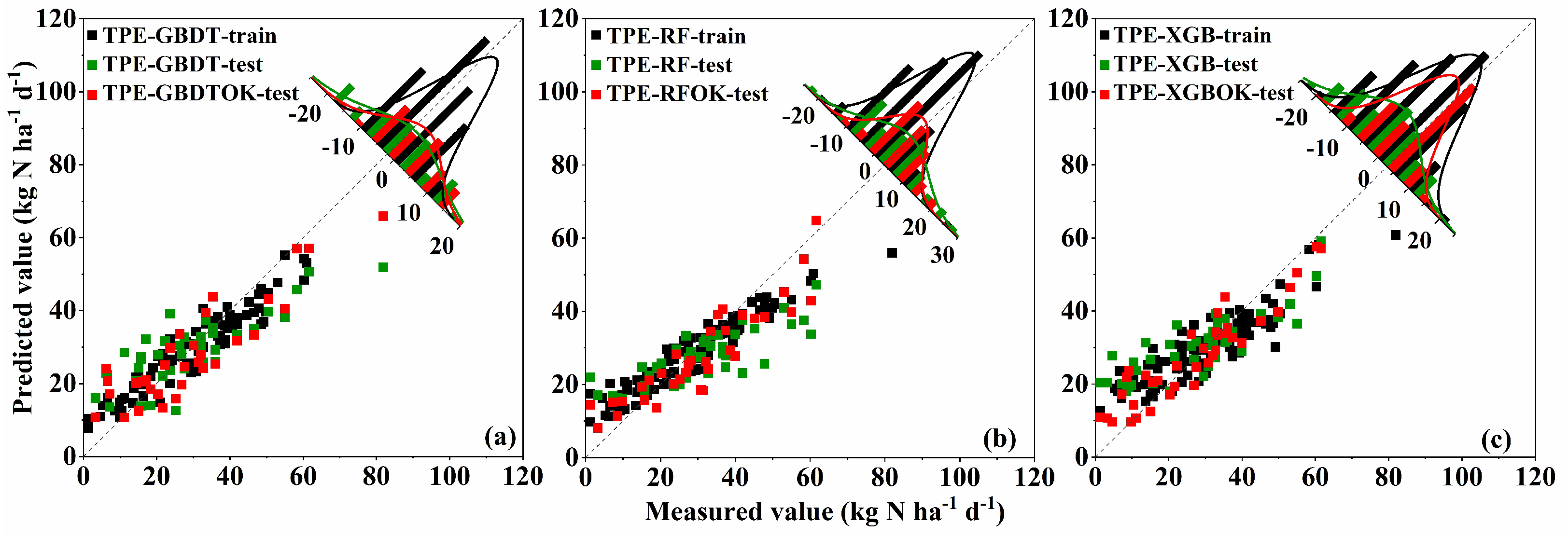
The scatter and residual distribution of the measured and predicted values of soil NH3 concentration and the regression accuracy of the model are shown in Figure 8 and Table 5, respectively. The spatial prediction accuracies of the TPE-optimized machine learning model for soil NH3 fluxes are TPE–XGB (RMSE = 8.13 kg N ha−1 d−1 and R2 = 74.22%) > TPE-RF (RMSE = 8.85 kg N ha−1 d−1 and R2 = 71.78%) > TPE–GBDT (RMSE = 10.40 kg N ha−1 d−1 and R2 = 65.90%) (Table 5). The TPE–XGB model had the strongest ability to fit the nonlinear relationship between soil NH3 flux and environmental variables in comparison with the other models. The residuals of the training sets of the three models satisfy the normal distribution, indicating a better-fitting performance of the models. The scatter distribution of the test set of the TPE–GBDT model is dispersive, and the prediction accuracy is significantly affected by the anomalous samples. In addition, the fitting curves of the residuals of the test sets of the three models show left skewness (i.e., the predicted residuals are concentrated in the negative region), indicating that the model predictions are underestimated.
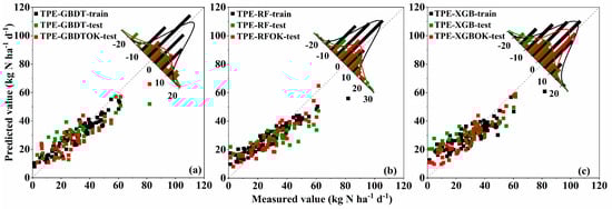
Figure 8.
Scatter error plot of soil NH3 flux measured value vs. predicted value using (a) TPE–GBDT–OK, (b) TPE–RF–OK, and (c) TPE–XGB–OK models.
Table 5.
The accuracy evaluation of prediction models for soil NH3 flux.
3.2.3. The Semi-Variation Analysis of Residual Values from TPE–GBDT, TPE–RF, and TPE–XGB Models
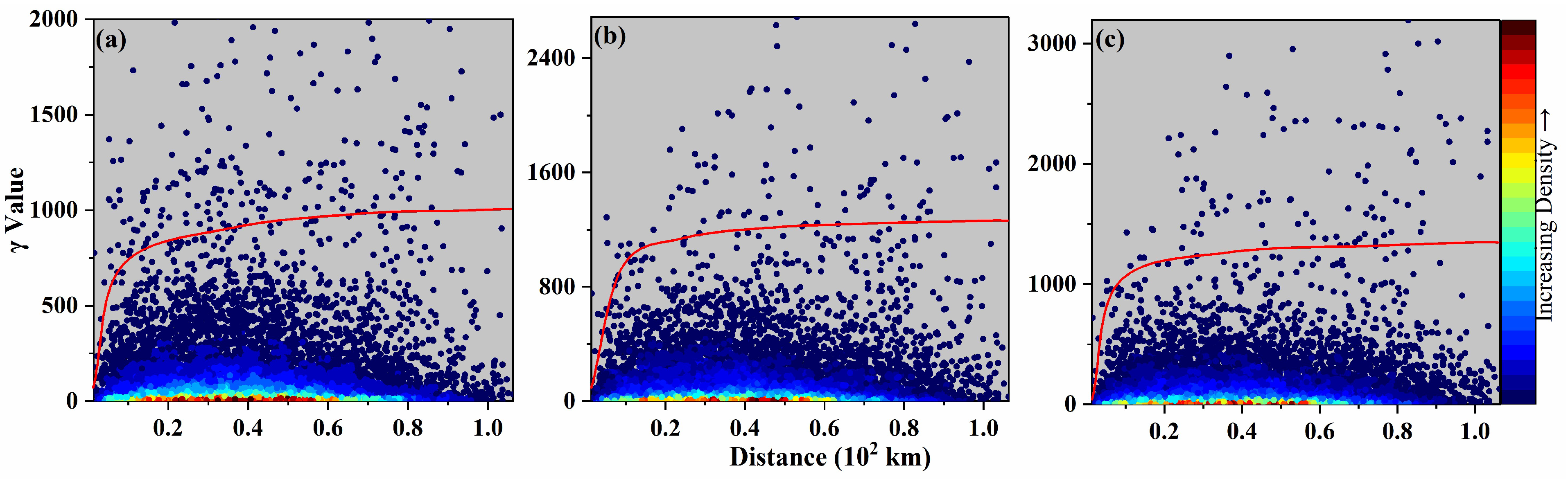
Furthermore, the spatial semi-variation characteristics of the predicted residuals of the three models were analyzed in ArcGIS 10.7 software. The nugget effect is an important indicator used for measuring the spatial variability of the sample points, usually divided into low spatial dependence (NE ≤ 25%) and moderate spatial dependence (25% ≤ NE ≤ 75%) [61]. The NE of the soil NH3 flux of residual sample points for OK exhibited moderate spatial dependence, making it appropriate for kriging interpolation (Table 6). In the process of semivariogram analysis, the residual sampling points showed a nonuniform distribution, and the semivariogram value (γ) tended to be stable as the step size increased. The residual sample points have the highest density (i.e., the strongest spatial autocorrelation) between the distance (h) from 0.1 to 0.6 (Figure 9).
Table 6.
The semi-variation analysis of residuals of soil NH3 using TPE–GBDT, TPE–RF, and TPE–XGB models.
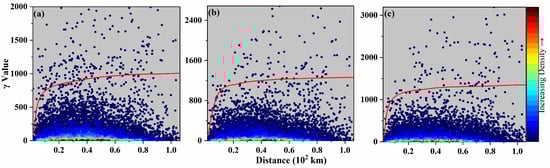
Figure 9.
Cumulative semivariograms of residual points of (a) TPE–GBDT, (b) TPE–RF, and (c) TPE–XGB models.
3.2.4. Spatial Prediction and Mapping Using the TPE–ML–OK Method
As shown in Table 5, the combined prediction accuracy of the TPE–ML–OK method was higher than that of the monotonic machine learning model, and the three integration models characterized more than 75% of the spatial variability (R2) of soil NH3 fluxes. Moreover, the test set scattering points of the three integration models were more compactly distributed near the diagonal, and their residuals were closer to normal distribution and concentrated in the low-value region (Figure 8). The TPE–XGB–OK model exhibited the highest prediction accuracy (i.e., RMSE = 6.42 kg N ha−1 d−1, and R2 = 85.97%) in comparison with the other models, which indicated that the TPE–XGB–OK model could explain the linear and nonlinear relationships between soil NH3 and environmental variables. The above results exhibited that the ML models assisted by the TPE algorithm have a more uniform distribution of residuals with fewer extremes, and the smoothing effect of residual kriging interpolation promotes the higher prediction accuracy of the TPE–ML–OK method.
Figure 10 shows soil NH3 fluxes spatially mapped using three integration prediction models. The predicted range of the TPE–XGB–OK model (0.7–82.36 kg N ha−1 d−1) was closest to the range of the true values (1.31–81.89 kg N ha−1 d−1), whereas the mapping results of the TPE-GBDT-OK model appeared to feature a significant underestimation. The spatial mapping results of the three hybrid models were similar, with the TPE–XGB–OK model predicting a more natural spatial excess of soil NH3 fluxes. Soil NH3 fluxes in the study area were smaller in the south as a whole, and the areas with larger concentrations were mainly distributed in the central and northeastern of the study area. Especially near the Yellow River estuary, the high soil NH3 fluxes may be influenced by river transport effects or soil moisture.
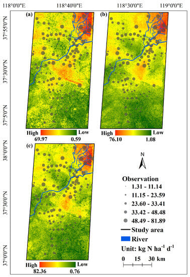
Figure 10.
Spatial distribution of soil NH3 fluxes in the study area based on (a) TPE–GBDT–OK, (b) TPE–RF–OK, and (c) TPE–XGB–OK models.
4. Discussion
4.1. Importance Analysis of Environmental Variables on Soil NH3
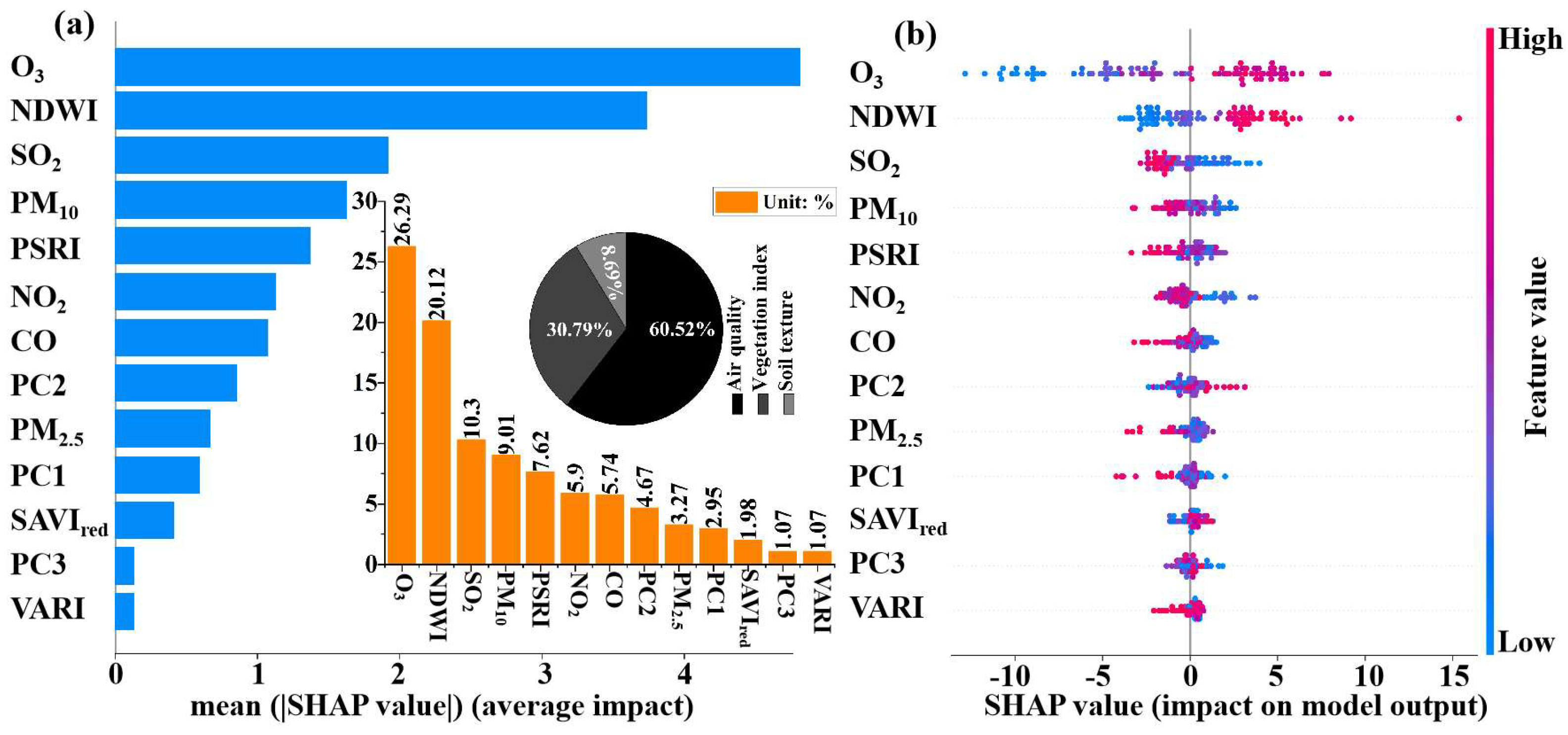
SHAP analysis is used to explore the contribution trajectory of environmental variables in the prediction process based on the TPE–XGB model. As shown in Figure 11, among the three types of variables of vegetation, air quality, and soil texture, the most significant impact on the spatial variability of soil NH3 flux is air quality (i.e., cumulative contribution ratio is 60.52%), followed by vegetation (i.e., cumulative contribution ratio is 30.79%) (Figure 11a). Among all the environmental variables, O3 had the highest contribution to the prediction accuracy of soil NH3 (26.29%), and the cumulative importance contribution rate of the first five environmental variables exceeded 70%. The mean SHAP values of other environmental variables such as VARI, PC3, SAVIred, PC1, and PM2.5 were all below 1, which had a low importance on the prediction accuracy of soil NH3. The characterization of the driving force of environmental variables on soil NH3 flux at each sample point is shown in Figure 11b. The SHAP value of the samples with low O3 value is negative (i.e., the closer the color is to blue, the smaller the feature value is), and the samples with high O3 value have positive SHAP values (i.e., the closer the color is to red, the larger the feature value is). That is, O3 shows a significant positive driving effect on soil NH3 (i.e., an increase in O3 content in the air will promote the emission of soil NH3). Similarly, NDWI is also positively correlated with soil NH3. Inversely, the SHAP values corresponding to the samples with higher SO2, PM10, and PSRI values are negative. This result indicates that these variables had a negative driving effect on soil NH3.

Figure 11.
The SHAP analysis: (a) a standard bar chart obtained using the absolute value of the mean SHAP values of each variable, and (b) the SHAP values of the environmental variable in each sampling point using the TPE–XGB model. The SHAP value is higher than 0, which means that the variable responds to a positive influence on the soil NH3; otherwise, it has a negative influence.
4.2. The Mechanism of Influence of Environmental Variables on Soil NH3
Air quality is an important driving factor affecting NH3 fluxes from farmland soil in the study area. According to the SHAP analysis, the positive driving effect of O3 is the most significant. The mechanism of the response of O3 on soil N emissions is that it changes soil microbial activity through plant-mediated processes, which may have an important impact on net gas fluxes, because it does not penetrate the soil and has a direct impact on the components of the soil ecosystem [62]. For example, elevated O3 concentrations reduce net photosynthesis [63,64] and dry matter accumulation [65] by oxidatively damaging plant cell membranes and chloroplasts [63,64,66,67,68,69], which in turn alters the soil subsurface processes of plant root respiration and microbial activity [41,70,71,72,73], ultimately affecting the nitrogen (N) and carbon (C) cycles in soil [74,75] and greenhouse gas emissions (CO2, CH4, N2O, etc.) [76]. Recio et al. (2020) found that the high O3 concentration significantly reduced the absorption of NH3 and other emissions from soil by plants [9], thereby increasing the emission of some nitrogen gases. For example, the increase in O3 concentration will significantly increase the peak CH4 flux of wheat and rice [77], and even under the highest O3 concentration treatment, the cumulative emission of soil N2O will double [78]. With the increase in O3 concentration, the emission of N element gas also increased, which proved that O3 was a positive driving force for soil NH3 in this study.
In addition to air quality variables, soil moisture (NDWI) also had a significant effect on the spatial variability of soil NH3 flux in this study. On the one hand, soil moisture has a significant positive effect and sensitivity on soil NH3 emission [79,80]. For example, since soil NH3 flux is a physical process affected by the concentration of -N in soil solution [81], the increase in soil moisture will promote the diffusion of NH3 in soil, resulting in the increase of soil NH3 emission [79,82,83,84]. On the other hand, soil moisture controls the loss of NH3 by affecting urea-hydrolyzing microorganisms and urease activity [84,85,86]. The increase in the liquid diffusion rate in moist soil is beneficial to the absorption of matrix by microorganisms and promotes the diffusion of NH3 in soil (and the emission of soil NH3) [87]. This is similar to the results of this study. In the estuary area of the Yellow River in the northeast of the study area, due to the dense river network and the high moisture of the farmland soil, the soil NH3 concentration is high. In addition, other variables such as soil salinity, soil pH, temperature, and wind speed may also affect soil NH3 emissions [88,89,90,91].
4.3. Limitations
We developed a TPE–ML–OK method with Sentinel-2 remote sensing image and air quality data to predict the spatial distribution of NH3 in farmland soil. However, this study has some limitations that should be considered in the future. First, the environmental variables that dominate soil NH3 emissions under different land use types are significantly different. For example, differences in land cover and land management methods can significantly affect soil NH3 emissions. The highest total environmental NHx concentration in rural areas may be related to intensive agricultural activities (such as fertilization and irrigation) [92], while soil pH, mineral nitrogen content, soil temperature, and humidity in the agro-pastoral ecotone play a key role in regulating NH3 emissions [93].
Second, the high fertilization rate was a significant environmental variable that promoted soil NH3 emission. The accumulation of chemical fertilizers and organic fertilizers in the soil leads to an increase in the transfer of NH3 from the liquid phase to the gas phase and promotes the volatilization of NH3 [94,95]. For example, the high nitrogen fertilizer input will lead to an increase in NH3 volatilization, and the more nitrogen fertilizer applied, the more nitrogen loss caused by NH3 volatilization [96], which becomes the main source of ammonia emission increasing in the atmosphere [97]. On the contrary, the volatilization of NH3 is limited by washing the fertilizer into the deep soil so that it is adsorbed [98].
Third, the influence of meteorological conditions on soil NH3 emission should be considered. NH3 volatilization loss is affected by many factors, such as temperature, precipitation, and precipitation [88,89,90,91,99]. Cold weather is not conducive to the emission of NH3, and strong precipitation may also lead to the removal of ammonia in the soil, resulting in a low concentration of ammonia discharged from the soil [97]. With the increase in temperature, the initial emission of NH3 will increase. When the temperature exceeds the optimum level, NH3 volatilization may not be significantly affected by temperature changes. [95] Other soil properties also have positive or negative effects on NH3 emissions. For example, acidic loam is also not conducive to the emission of NH3 [97]; that is, soil pH is positively correlated with NH3 emission, and soil pH will affect the content of -N in the ammonia conversion reaction system, thus affecting the emission process of soil NH3 [93]. The higher the soil pH, the more NH3 volatilization [96]. The increase in clay content leads to decreased electrical conductivity, which limits the vertical transfer of nitrogen [95].
In addition, spatial interpolation is used to obtain the spatial continuity distribution of air quality stations, which is a stable and effective method in small-scale areas. However, in future studies, improving the spatial accuracy of air quality data should be considered in order to further improve its response to the spatial prediction of soil NH3 and reduce the uncertainty of prediction. For example, in large-scale areas, the use of aerosol images (such as MODIS and Himawari) and a large number of monitoring station data, combined with machine learning models, can effectively improve the spatial prediction accuracy of air quality, thereby reducing the uncertainty of air quality variables in predicting soil NH3 flux.
5. Conclusions
In this study, we developed an integration method to predict the spatial distribution of NH3 flux in farmland soil. The GBDT, RF, and XGB models assisted by the TPE algorithm found the optimal hyperparameters, and the probability that the optimal hyperparameters appear in the dense sampling area of TPE iterations. Compared with a single ML model, the three integration models exhibited higher predicted performance for the spatial variability of soil NH3 fluxes. Moreover, the TPE–XGB–OK model effectively explained the linear and nonlinear relationships between environmental variables and soil NH3. The areas with high flux of NH3 in farmland soil were concentrated centrally and in the northeast. Further importance analysis of environmental variables exhibited that air quality and soil moisture have a significant positive driving effect on soil NH3. That is, O3 promotes soil NH3 flux by altering the soil subsurface processes of plant root respiration and microbial activity, and soil moisture also has a direct promotion effect on soil NH3 emission. In the future, the integration method can be generalized to spatio–temporal fusion prediction, supporting global warming alleviation and high-quality agriculture development in coastal areas.
Author Contributions
Conceptualization, Y.S.; methodology, D.Z.; software, D.Z. and M.Y.; validation, M.Y. and Z.Z.; formal analysis, Y.S. and W.D.; investigation, M.L.; resources, Y.S. and M.L.; data curation, M.Y. and Z.D.; writing—original draft, Y.S. and D.Z.; visualization, K.Y.; writing—review and editing, Z.S. and D.S.; supervision, Y.S.; project administration, Y.S.; funding acquisition, Y.S. and M.L. All authors have read and agreed to the published version of the manuscript.
Funding
This research was funded by the Shandong Provincial Natural Science Foundation (ZR2020QD013), the National Natural Science Foundation of China (42071419), and the Agricultural Science and Technology Innovation Program (ASTIP No. CAAS-ZDRW202201).
Institutional Review Board Statement
Not applicable.
Informed Consent Statement
Not applicable.
Data Availability Statement
The Sentinel-2 remote sensing image (23 September 2022) comes from the European Space Agency (https://scihub.copernicus.eu/, (accessed on 12 November 2022)). The air quality data comes from the Dongying air quality real-time publishing system (http://218.58.213.53:8081/dyfb_air/fb_web, (accessed on 10 November 2022)).
Conflicts of Interest
The authors declare no conflict of interest.
References
- Liu, M.; Huang, X.; Song, Y.; Tang, J.; Cao, J.; Zhang, X.; Zhang, Q.; Wang, S.; Xu, T.; Kang, L.; et al. Ammonia emission control in China would mitigate haze pollution and nitrogen deposition, but worsen acid rain. Proc. Natl. Acad. Sci. USA 2019, 116, 7760–7765. [Google Scholar] [CrossRef]
- Zhang, Z.; Yan, Y.; Kong, S.; Deng, Q.; Qin, S.; Yao, L.; Zhao, T.; Qi, S. Benefits of refined NH3 emission controls on PM2.5 mitigation in Central China. Sci. Total Environ. 2021, 814, 151957. [Google Scholar] [CrossRef] [PubMed]
- Erisman, J.W.; Sutton, M.A.; Galloway, J.; Klimont, Z.; Winiwarter, W. How a century of ammonia synthesis changed the world. Nat. Geosci. 2008, 1, 636–639. [Google Scholar] [CrossRef]
- Galloway, J.N.; Townsend, A.R.; Erisman, J.W.; Bekunda, M.; Cai, Z.; Freney, J.R.; Martinelli, L.A.; Seitzinger, S.P.; Sutton, M.A. Transformation of the Nitrogen Cycle: Recent Trends, Questions, and Potential Solutions. Science 2008, 320, 889–892. [Google Scholar] [CrossRef] [PubMed]
- Gu, B.; Ge, Y.; Ren, Y.; Xu, B.; Luo, W.; Jiang, H.; Gu, B.; Chang, J. Atmospheric Reactive Nitrogen in China: Sources, Recent Trends, and Damage Costs. Environ. Sci. Technol. 2012, 46, 9420–9427. [Google Scholar] [CrossRef] [PubMed]
- The IPCC Working Group. Climate Change 2013: The Physical Science Basis—Conclusions. Bull. Angew. Geol. 2013, 18, 5–19. [Google Scholar]
- Tian, H.; Xu, R.; Canadell, J.G.; Thompson, R.L.; Winiwarter, W.; Suntharalingam, P.; Davidson, E.A.; Ciais, P.; Jackson, R.B.; Janssens-Maenhout, G.; et al. Comprehensive Quantification of Global Nitrous Oxide Sources and Sinks. Nature 2020, 586, 248–256. [Google Scholar] [CrossRef]
- Sutton, M.A.; Reis, S.; Riddick, S.N.; Dragosits, U.; Nemitz, E.; Theobald, M.R.; Tang, Y.S.; Braban, C.F.; Vieno, M.; Dore, A.J.; et al. Towards a climate-dependent paradigm of ammonia emission and deposition. Philos. Trans. R. Soc. B Biol. Sci. 2013, 368, 20130166. [Google Scholar] [CrossRef]
- Recio, J.; Montoya, M.; Ginés, C.; Sanz-Cobena, A.; Alvarez, J.M. Joint mitigation of NH3 and N2O emissions by using two synthetic inhibitors in an irrigated cropping soil. Geoderma 2020, 373, 114423. [Google Scholar] [CrossRef]
- Nelson, A.J.; Koloutsou-Vakakis, S.; Rood, M.J.; Myles, L.; Lehmann, C.; Bernacchi, C.; Balasubramanian, S.; Joo, E.; Heuer, M.; Vieira-Filho, M.; et al. Season-long ammonia flux measurements above fertilized corn in central Illinois, USA, using relaxed eddy accumulation. Agric. For. Meteorol. 2017, 239, 202–212. [Google Scholar] [CrossRef]
- Walker, J.T.; Jones, M.R.; Bash, J.O.; Myles, L.; Meyers, T.; Schwede, D.; Herrick, J.; Nemitz, E.; Robarge, W. Processes of ammonia air–surface exchange in a fertilized Zea mays canopy. Biogeosciences 2013, 10, 981–998. [Google Scholar] [CrossRef]
- Bao, Z.; Xu, H.; Li, K.; Chen, L.; Zhang, X.; Wu, X. Effects of NH3 on secondary aerosol formation from toluene/NOx photo-oxidation in different O3 formation regimes. Atmos. Environ. 2021, 9, 261. [Google Scholar] [CrossRef]
- Gu, M.; Pan, Y.; Sun, Q.; Walters, W.W.; Song, L.; Fang, Y. Is fertilization the dominant source of ammonia in the urban atmosphere? Sci. Total Environ. 2022, 838, 155890. [Google Scholar] [CrossRef] [PubMed]
- Bhattarai, N.; Wang, S.; Xu, Q.; Dong, Z.; Chang, X.; Jiang, Y.; Zheng, H. Nitrogen isotopes suggest agricultural and non-agricultural sources contribute equally to NH3 and NH4+ in urban Beijing during December 2018. Environ. Pollut. 2023, 326, 121455. [Google Scholar] [CrossRef] [PubMed]
- Li, K.; Chen, L.; White, S.J.; Yu, H.; Wu, X.; Gao, X.; Azzi, M.; Cen, K. Smog chamber study of the role of NH3 in new particle formation from photo-oxidation of aromatic hydrocarbons. Sci. Total Environ. 2018, 619–620, 927–937. [Google Scholar] [CrossRef]
- Na, K.; Song, C.; Cocker, D.R., III. Formation of secondary organic aerosol from the reaction of styrene with ozone in the presence and absence of ammonia and water. Atmos. Environ. 2006, 40, 1889–1900. [Google Scholar] [CrossRef]
- Goovaerts, P. Geostatistics in soil science: State-of-the-art and perspectives. Geoderma 1999, 89, 1–45. [Google Scholar] [CrossRef]
- Yfantis, E.A.; Flatman, G.T.; Behar, J.V. Efficiency of kriging estimation for square, triangular, and hexagonal grids. Math. Geol. 1987, 19, 183–205. [Google Scholar] [CrossRef]
- Di Martino, R.M.R.; Capasso, G.; Camarda, M. Spatial domain analysis of carbon dioxide from soils on Vulcano Island: Implications for CO2 output evaluation. Chem. Geol. 2016, 444, 59–70. [Google Scholar] [CrossRef]
- Oliver, M.A.; Webster, R. A tutorial guide to geostatistics: Computing and modelling variograms and kriging. Catena 2014, 113, 56–69. [Google Scholar] [CrossRef]
- Mirzaei, M.; Gorji Anari, M.; Diaz-Pines, E.; Saronjic, N.; Mohammed, S.; Szabo, S.; Nasir Mousavi, S.M.; Caballero-Calvo, A. Assessment of soil CO2 and NO fluxes in a semi-arid region using machine learning approaches. J. Arid Environ. 2023, 211, 104947. [Google Scholar] [CrossRef]
- Abbasi, N.A.; Hamrani, A.; Madramootoo, C.A.; Zhang, T.; Tan, C.S.; Goyal, M.K. Modelling carbon dioxide emissions under a maize-soy rotation using machine learning. Biosyst. Eng. 2021, 212, 1–18. [Google Scholar] [CrossRef]
- Meinshausen, N.; Ridgeway, G. Quantile Regression Forests. J. Mach. Learn. Res. 2006, 7, 983–999. [Google Scholar]
- Warner, D.L.; Guevara, M.; Inamdar, S.; Vargas, R. Upscaling soil-atmosphere CO2 and CH4 fluxes across a topographically complex forested landscape. Agric. For. Meteorol. 2019, 264, 80–91. [Google Scholar] [CrossRef]
- Yan, H.; Yan, K.; Ji, G. Optimization and prediction in the early design stage of office buildings using genetic and XGBoost algorithms. Build. Environ. 2022, 218, 109081. [Google Scholar] [CrossRef]
- Zhu, X.; Chu, J.; Wang, K.; Wu, S.; Yan, W.; Chiam, K. Prediction of rockhead using a hybrid N-XGBoost machine learning framework. J. Rock Mech. Geotech. Eng. 2021, 13, 1231–1245. [Google Scholar] [CrossRef]
- Yun, K.K.; Yoon, S.W.; Won, D. Prediction of stock price direction using a hybrid GA-XGBoost algorithm with a three-stage feature engineering process. Expert Syst. Appl. 2021, 186, 115716. [Google Scholar] [CrossRef]
- Guo, P.; Li, M.; Luo, W.; Tang, Q.; Liu, Z.; Lin, Z. Digital mapping of soil organic matter for rubber plantation at regional scale: An application of random forest plus residuals kriging approach. Geoderma 2015, 237–238, 49–59. [Google Scholar] [CrossRef]
- Demyanov, V.; Soltani, S.; Kanevski, M.; Canu, S.; Maignan, M.; Savelieva, E.; Timonin, V.; Pisarenko, V. Wavelet analysis residual kriging vs. neural network residual kriging. Stoch. Environ. Res. Risk Assess. 2001, 15, 18–32. [Google Scholar] [CrossRef]
- Song, Y.-Q.; Yang, L.-A.; Li, B.; Hu, Y.-M.; Wang, A.-L.; Zhou, W.; Cui, X.; Liu, Y.-L. Spatial Prediction of Soil Organic Matter Using a Hybrid Geostatistical Model of an Extreme Learning Machine and Ordinary Kriging. Sustainability 2017, 9, 754. [Google Scholar] [CrossRef]
- Demyanov, V.; Kanevsky, M.; Chernov, S.; Savelieva, E.; Timonin, V. Neural Network Residual Kriging Application for Climatic Data. J. Geogr. Inf. Decis. Anal. 1998, 2, 215–232. [Google Scholar]
- Kanevski, M.; Pozdnoukhov, A.; Timonin, V. Machine Learning for Spatial Environmental Data: Theory, Applications, and Software; EPFL Press: Lausanne, Switzerland, 2009; pp. 1–371. [Google Scholar]
- Seo, Y.; Kim, S.; Singh, V.P. Estimating Spatial Precipitation Using Regression Kriging and Artificial Neural Network Residual Kriging (RKNNRK) Hybrid Approach. Water Resour. Manag. 2015, 29, 2189–2204. [Google Scholar] [CrossRef]
- Kanevski, M.; Parkin, R.; Pozdnukhov, A.; Timonin, V.; Maignan, M.; Demyanov, V.; Canu, S. Environmental data mining and modeling based on machine learning algorithms and geostatistics. Environ. Modell. Softw. 2004, 19, 845–855. [Google Scholar] [CrossRef]
- Kanevski, M.; Arutyunyan, R.; Bolshov, L.; Demyanov, V.; Maignan, M. Artificial Neural Networks and Spatial Estimation of Chernobyl Fallout. Geoinformatica 1996, 7, 5–11. [Google Scholar] [CrossRef]
- Chen, T.H.; Hsu, Y.C.; Zeng, Y.T.; Lung, S.C.C.; Su, H.J.; Chao, H.J.; Wu, C.D. A hybrid kriging/land-use regression model with Asian culture-specific sources to assess NO2 spatial-temporal variations. Environ. Pollut. 2020, 259, 113875. [Google Scholar] [CrossRef] [PubMed]
- Yang, T. Response of Soil Ammonia Volatilization and Canopy Ammonia Exchange to Conservation Tillage in Spring Maize Field of Guanzhong Region; Northwest A & F University: Xianyang, China, 2021; p. 77. [Google Scholar]
- Thottathil, S.D.; Reis, P.C.J.; Prairie, Y.T. Magnitude and Drivers of Oxic Methane Production in Small Temperate Lakes. Environ. Sci. Technol. 2022, 56, 11041–11050. [Google Scholar] [CrossRef]
- Hua, S.; Qing, W.; Guangxing, W.; Hui, L.; Peng, L.; Jiping, L.; Siqi, Z.; Xiaoyu, X.; Lanxiang, R. Optimizing kNN for Mapping Vegetation Cover of Arid and Semi-Arid Areas Using Landsat Images. Remote Sens. 2018, 10, 1248. [Google Scholar]
- Huete, A.R.; Huete, A.R. A soil-adjusted vegetation index (SAVI). Remote Sens. Environ. 1988, 25, 295–309. [Google Scholar] [CrossRef]
- Mccrady, J.K.; Andersen, C.P. The effect of ozone on below-ground carbon allocation in wheat. Environ. Pollut. 2000, 107, 465–472. [Google Scholar] [CrossRef]
- Merzlyak, M.N.; Gitelson, A.A.; Chivkunova, O.B.; Rakitin, V.Y. Non-destructive optical detection of pigment changes during leaf senescence and fruit ripening. Physiol. Plant. 1999, 106, 135–141. [Google Scholar] [CrossRef]
- Xiang, X.; Du, J.; Jacinthe, P.A.; Zhao, B.; Zhou, H.; Liu, H.; Song, K. Integration of tillage indices and textural features of sentinel-2a multispectral images for maize residue cover estimation. Soil Tillage Res. 2022, 221, 105405. [Google Scholar] [CrossRef]
- Koley, S.; Jeganathan, C. Sentinel 1 and Sentinel 2 for Cropland Mapping with Special Emphasis on the usability of Textural and Vegetation Indices. Adv. Space Res. 2021, 69, 1768–1785. [Google Scholar] [CrossRef]
- Duan, M.; Zhang, X. Using remote sensing to identify soil types based on multiscale image texture features. Comput. Electron. Agric. 2021, 187, 106272. [Google Scholar] [CrossRef]
- Haralick, R.M.; Shanmugam, K.; Dinstein, I. Textural features for image classification. IEEE Trans. Syst. Man Cybern. 1973, 3, 610–621. [Google Scholar] [CrossRef]
- Kupidura, P. The comparison of different methods of texture analysis for their efficacy for land use classification in satellite imagery. Remote Sens. 2019, 11, 1233. [Google Scholar] [CrossRef]
- Lu, H.; Liu, C.; Li, N.; Fu, X.; Li, L. Optimal segmentation scale selection and evaluation of cultivated land objects based on high-resolution remote sensing images with spectral and texture features. Environ. Sci. Pollut. Res. 2021, 28, 27067–27083. [Google Scholar] [CrossRef]
- Cutler, D.R.; Edwards, T.C.J.; Beard, K.H.; Cutler, A.; Hess, K.T.; Gibson, J.; Lawler, J.J. Random forests for classification in ecology. Ecology 2007, 88, 2783–2792. [Google Scholar] [CrossRef]
- Jiang, F.; Kutia, M.; Sarkissian, A.J.; Lin, H.; Long, J.; Sun, H.; Wang, G. Estimating the Growing Stem Volume of Coniferous Plantations Based on Random Forest Using an Optimized Variable Selection Method. Sensors 2020, 20, 7248. [Google Scholar] [CrossRef]
- Chen, T.; Guestrin, C. XGBoost: A Scalable Tree Boosting System; ACM: Ithaca, NY, USA, 2016; pp. 785–794. [Google Scholar]
- Ha, N.T.; Manley-Harris, M.; Pham, T.D.; Hawes, I. The use of radar and optical satellite imagery combined with advanced machine learning and metaheuristic optimization techniques to detect and quantify above ground biomass of intertidal seagrass in a New Zealand estuary. Int. J. Remote Sens. 2021, 42, 4712–4738. [Google Scholar] [CrossRef]
- Albaqami, H.; Hassan, G.M.; Subasi, A.; Datta, A. Automatic detection of abnormal EEG signals using wavelet feature extraction and gradient boosting decision tree. Biomed. Signal Process. Control 2020, 70, 102957. [Google Scholar] [CrossRef]
- Nguyen, T.T.; Ngo, H.H.; Guo, W.; Chang, S.W.; Nguyen, D.D.; Nguyen, C.T.; Zhang, J.; Liang, S.; Bui, X.T.; Hoang, N.B. A low-cost approach for soil moisture prediction using multi-sensor data and machine learning algorithm. Sci. Total Environ. 2022, 833, 155066. [Google Scholar] [CrossRef] [PubMed]
- Zhou, T.; Geng, Y.; Chen, J.; Liu, M.; Haase, D.; Lausch, A. Mapping soil organic carbon content using multi-source remote sensing variables in the Heihe River Basin in China. Ecol. Indic. 2020, 114, 106288. [Google Scholar] [CrossRef]
- Zhou, T.; Geng, Y.; Chen, J.; Pan, J.; Lausch, A. High-resolution digital mapping of soil organic carbon and soil total nitrogen using DEM derivatives, Sentinel-1 and Sentinel-2 data based on machine learning algorithms. Sci. Total Environ. 2020, 729, 138244. [Google Scholar] [CrossRef] [PubMed]
- Ozaki, Y.; Tanigaki, Y.; Watanabe, S.; Onishi, M. Multiobjective tree-structured parzen estimator for computationally expensive optimization problems. In Proceedings of the 2020 Genetic and Evolutionary Computation Conference, Cancún, Mexico, 8–12 July 2020; Volume 73, pp. 1209–1250. [Google Scholar]
- Webster, R.; Oliver, M.A. Statistics for earth and environmental scientists. In Geostatistics for Environmental Scientists, 2nd ed.; John Wiley & Sons: New York, NY, USA, 2008; Volume 41, pp. 487–489. [Google Scholar]
- Mirzaee, S.; Ghorbani-Dashtaki, S.; Mohammadi, J.; Asadi, H.; Asadzadeh, F. Spatial variability of soil organic matter using remote sensing data. CATENA 2016, 145, 118–127. [Google Scholar] [CrossRef]
- Chen, C.; Seo, H. Prediction of rock mass class ahead of TBM excavation face by ML and DL algorithms with Bayesian TPE optimization and SHAP feature analysis. Acta Geotech. 2023, 18, 3825–3848. [Google Scholar] [CrossRef]
- Cambardella, C.A.; Moorman, T.B.; Novak, J.M.; Parkin, T.B.; Konopka, A.E. Field-Scale Variability of Soil Properties in Central Iowa Soils. Soil Sci. Soc. Am. J. 1994, 58, 1501–1511. [Google Scholar] [CrossRef]
- Blum, U.; Tingey, D.T. A study of the potential ways in which ozone could reduce root growth and nodulation of soybean. Atmos. Environ. 1977, 11, 737–739. [Google Scholar] [CrossRef]
- Nie, G.Y.; Tomasevic, M.; Baker, N.R. Effects of ozone on the photosynthetic apparatus and leaf proteins during leaf development in wheat. Plant Cell Environ. 2010, 16, 643–651. [Google Scholar] [CrossRef]
- Karberg, N.J.; Pregitzer, K.S.; King, J.S.; Friend, A.L.; Wood, J.R. Soil carbon dioxide partial pressure and dissolved inorganic carbonate chemistry under elevated carbon dioxide and ozone. Oecologia 2005, 142, 296–306. [Google Scholar] [CrossRef]
- Nouchi, I.; Ito, O.; Harazono, Y.; Kobayashi, K. Effects of chronic ozone exposure on growth, root respiration and nutrient uptake of rice plants. Environ. Pollut. 1991, 74, 149–164. [Google Scholar] [CrossRef]
- Shi, G.; Yang, L.; Wang, Y.; Kobayashi, K.; Zhu, J.; Tang, H.; Pan, S.; Chen, T.; Liu, G.; Wang, Y. Impact of elevated ozone concentration on yield of four Chinese rice cultivars under fully open-air field conditions. Agric. Ecosyst. Environ. 2009, 131, 178–184. [Google Scholar] [CrossRef]
- Maggs, R.; Ashmore, M.R. Growth and yield responses of Pakistan rice (Oryza sativa L.) cultivars to O3 and NO2. Environ. Pollut. 1998, 103, 159–170. [Google Scholar] [CrossRef]
- Kobayashi, K.; Okada, M. Effects of ozone on the light use of rice (Oryza sativa L.) plants. Agric. Ecosyst. Environ. 1995, 53, 1–12. [Google Scholar] [CrossRef]
- Feng, Z.; Kobayashi, K.; Ainsworth, E.A. Impact of elevated ozone concentration on growth, physiology, and yield of wheat (Triticum aestivum L.): A meta-analysis. Global Chang. Biol. 2008, 14, 2696–2708. [Google Scholar] [CrossRef]
- Kou, T.J.; Yu, W.W.; Zhu, J.G.; Zhu, X.K. Effects of ozone pollution on the accumulation and distribution of dry matter and biomass carbon of different varieties of wheat. Huan Jing Ke Xue = Huanjing Kexue 2012, 33, 2862–2867. [Google Scholar] [PubMed]
- Kanerva, T.; Palojrvi, A.; Rm, K.; Ojanper, K.; Esala, M.; Manninen, S. A 3-year exposure to CO2 and O3 induced minor changes in soil N cycling in a meadow ecosystem. Plant Soil 2006, 286, 61–73. [Google Scholar] [CrossRef]
- Jones, T.G.; Freeman, C.; Lloyd, A.; Mills, G. Impacts of elevated atmospheric ozone on peatland below-ground DOC characteristics. Ecol. Eng. 2009, 35, 971–977. [Google Scholar] [CrossRef]
- Fiscus, E.L.; Booker, F.L.; Burkey, K.O. Crop responses to ozone: Uptake, modes of action, carbon assimilation and partitioning. Plant Cell Environ. 2010, 28, 997–1011. [Google Scholar] [CrossRef]
- Larson, J.L.; Zak, D.R.; Sinsabaugh, R.L. Extracellular Enzyme Activity Beneath Temperate Trees Growing Under Elevated Carbon Dioxide and Ozone. Soil Sci. Soc. Am. J. 2002, 66, 1848–1856. [Google Scholar] [CrossRef]
- Islam, K.R.; Mulchi, C.L.; Ali, A.A. Interactions of tropospheric CO2 and O3 enrichments and moisture variations on microbial biomass and respiration in soil. Global Chang. Biol. 2001, 6, 255–265. [Google Scholar] [CrossRef]
- Lu, Y.; Conrad, R. In situ stable isotope probing of methanogenic archaea in the rice rhizosphere. Science 2005, 309, 1088–1090. [Google Scholar] [CrossRef] [PubMed]
- Kou, T.J.; Cheng, X.H.; Zhu, J.G.; Xie, Z.B. The influence of ozone pollution on CO2, CH4, and N2O emissions from a Chinese subtropical rice–wheat rotation system under free-air O3 exposure. Agric. Ecosyst. Environ. 2015, 204, 72–81. [Google Scholar] [CrossRef]
- Sánchez-Martín, L.; Bermejo-Bermejo, V.; García-Torres, L.; Alonso, R.; de la Cruz, A.; Calvete-Sogo, H.; Vallejo, A. Nitrogen soil emissions and belowground plant processes in Mediterranean annual pastures are altered by ozone exposure and N-inputs. Atmos. Environ. 2017, 165, 12–22. [Google Scholar] [CrossRef]
- Yang, Y.; Zhou, C.; Li, N.; Han, K.; Meng, Y.; Tian, X.; Wang, L. Effects of conservation tillage practices on ammonia emissions from Loess Plateau rain-fed winter wheat fields. Atmos. Environ. 2015, 104, 59–68. [Google Scholar] [CrossRef]
- Delon, C.; Galy-Lacaux, C.; Serça, D.; Loubet, B.; Camara, N.; Gardrat, E.; Saneh, I.; Fensholt, R.; Tagesson, T.; Le Dantec, V.; et al. Soil and vegetation-atmosphere exchange of NO, NH3, and N2O from field measurements in a semi arid grazed ecosystem in Senegal. Atmos. Environ. 2017, 156, 36–51. [Google Scholar] [CrossRef]
- Bosch-Serra, À.D.; Yagüe, M.R.; Teira-Esmatges, M.R. Ammonia emissions from different fertilizing strategies in Mediterranean rainfed winter cereals. Atmos. Environ. 2014, 84, 204–212. [Google Scholar] [CrossRef]
- Nye, P.H. Towards the quantitative control of crop production and quality. J. Plant Nutr. 1992, 15, 1129. [Google Scholar] [CrossRef]
- Pelster, D.E.; Watt, D.; Strachan, I.B.; Rochette, P.; Chantigny, M.H. Effects of Initial Soil Moisture, Clod Size, and Clay Content on Ammonia Volatilization after Subsurface Band Application of Urea. J. Environ. Qual. 2019, 48, 549–558. [Google Scholar] [CrossRef]
- Sommer, S.G.; Schjoerring, J.K.; Denmead, O.T. Ammonia emission from mineral fertilizers and fertilized crops. Adv. Agron. 2004, 82, 557–622. [Google Scholar]
- Sun, R.; Li, W.; Hu, C.; Liu, B. Long-term urea fertilization alters the composition and increases the abundance of soil ureolytic bacterial communities in an upland soil. FEMS Microbiol. Ecol. 2019, 95, fiz044. [Google Scholar] [CrossRef]
- Wali, P.; Kumar, V.; Singh, J.P. Effect of soil type, exchangeable sodium percentage, water content, and organic amendments on urea hydrolysis in some tropical Indian soils. Soil Res. 2003, 41, 1171–1176. [Google Scholar] [CrossRef]
- Blagodatsky, S.; Smith, P. Soil physics meets soil biology: Towards better mechanistic prediction of greenhouse gas emissions from soil. Soil Biol. Biochem. 2012, 47, 78–92. [Google Scholar] [CrossRef]
- Duan, Z.C.A.O.; Xiao, H. Effects of soil properties on ammonia volatilization. Soil Sci. Plant Nutr. 2000, 46, 845–852. [Google Scholar]
- Chen, S.; Li, D.; He, H.; Zhang, Q.; Lu, H.; Xue, L.; Feng, Y.; Sun, H. Substituting urea with biogas slurry and hydrothermal carbonization aqueous product could decrease NH3 volatilization and increase soil DOM in wheat growth cycle. Environ. Res. 2022, 214, 113997. [Google Scholar] [CrossRef]
- Hagner, M.; Räty, M.; Nikama, J.; Rasa, K.; Peltonen, S.; Vepsäläinen, J.; Keskinen, R. Slow pyrolysis liquid in reducing NH3 emissions from cattle slurry—Impacts on plant growth and soil organisms. Sci. Total Environ. 2021, 784, 147139. [Google Scholar] [CrossRef]
- Zheng, J.; Zhang, Y.; Ma, Y.; Ye, N.; Khalizov, A.F.; Yan, J. Radiatively driven NH3 release from agricultural field during wintertime slack season. Atmos. Environ. 2021, 247, 118228. [Google Scholar] [CrossRef]
- Zhang, Y.; Ma, X.; Tang, A.; Fang, Y.; Misselbrook, T.; Liu, X. Source Apportionment of Atmospheric Ammonia at 16 Sites in China Using a Bayesian Isotope Mixing Model Based on δ15N–NHx Signatures. Environ. Sci. Technol. 2023, 57, 6599–6608. [Google Scholar] [CrossRef]
- Wang, H.; Guo, R.; Tian, Y.; Cui, N.; Wang, X.; Wang, L.; Yang, Z.; Li, S.; Guo, J.; Shi, L.; et al. Arbuscular mycorrhizal fungi reduce NH3 emissions under different land-use types in agro-pastoral areas. Pedosphere 2023, 33, 1–24. [Google Scholar] [CrossRef]
- Zhan, X.; Adalibieke, W.; Cui, X.; Winiwarter, W.; Reis, S.; Zhang, L.; Bai, Z.; Wang, Q.; Huang, W.; Zhou, F. Improved estimates of ammonia emissions from global croplands. Environ. Sci. Technol. 2020, 55, 1329–1338. [Google Scholar] [CrossRef]
- Zhou, F.; Ciais, P.; Hayashi, K.; Galloway, J.; Kim, D.G.; Yang, C.; Li, S.; Liu, B.; Shang, Z.; Gao, S. Re-estimating NH3 Emissions from Chinese Cropland by a New Nonlinear Model. Environ. Sci. Technol. 2016, 50, 564–572. [Google Scholar] [CrossRef]
- Bi, S.; Luo, X.; Chen, Z.; Li, P.; Yu, C.; Liu, Z.; Peng, X. Fate of fertilizer nitrogen and residual nitrogen in paddy soil in Northeast China. J. Integr. Agric. 2023, in press. [Google Scholar] [CrossRef]
- Pan, Y.; Tian, S.; Zhao, Y.; Zhang, L.; Zhu, X.; Gao, J.; Huang, W.; Zhou, Y.; Song, Y.; Zhang, Q.; et al. Identifying ammonia hotspots in china using a national observation network. Environ. Sci. Technol. 2018, 52, 3926–3934. [Google Scholar] [CrossRef] [PubMed]
- Zhang, Y.; Benedict, K.B.; Tang, A.; Sun, Y.; Fang, Y.; Liu, X. Persistent nonagricultural and periodic agricultural emissions dominate sources of ammonia in urban Beijing: Evidence from 15N stable isotope in vertical profiles. Environ. Sci. Technol. 2019, 54, 102–109. [Google Scholar] [CrossRef] [PubMed]
- Kong, L.; Tang, X.; Zhu, J.; Wang, Z.; Pan, Y.; Wu, H.; Wu, L.; Wu, Q.; He, Y.; Tian, S.; et al. Improved inversion of monthly ammonia emissions in China based on the Chinese ammonia monitoring network and ensemble Kalman filter. Environ. Sci. Technol. 2019, 53, 12529–12538. [Google Scholar] [CrossRef] [PubMed]


Disclaimer/Publisher’s Note: The statements, opinions and data contained in all publications are solely those of the individual author(s) and contributor(s) and not of MDPI and/or the editor(s). MDPI and/or the editor(s) disclaim responsibility for any injury to people or property resulting from any ideas, methods, instructions or products referred to in the content. |
© 2023 by the authors. Licensee MDPI, Basel, Switzerland. This article is an open access article distributed under the terms and conditions of the Creative Commons Attribution (CC BY) license (https://creativecommons.org/licenses/by/4.0/).