Key Factors for Improving the Resolution of Mapped Sea Surface Height from Multi-Satellite Altimeters in the South China Sea

Abstract

A satellite altimeter measures sea surface height (SSH) along the nadir track. Multiple satellite altimeters have been in orbit, and the measurements been merged for mapping mesoscale eddies of ~100 km in size in the oceans. The capability of the mapped SSH for resolving mesoscale eddies depends on mapping algorithms. A two-dimensional variational (2DVAR) algorithm was implemented to generate mapped SSH at a grid size of 1/12° in the South China Sea. A range of comparisons were performed between the mapped SSH and the commonly used AVISO (Archiving, Validation, and Interpretation of Satellite Oceanographic satellite data) mapped SSH data product at a grid size of 1/8° and 1/4°. The effective resolution, which represents the spatial scale that the data can resolve, was examined. The effective resolution of the mapped SSH using the 2DVAR algorithm is approximately 100 km, while it is 250 km with the 1/8° and 1/4° AVISO data products. The difference in the effective resolution results from the difference in the background state and thus the background error. The result suggests that the effective resolution of the mapped data could be increased by choosing a background state so that the associated errors could have a smaller decorrelation length scale.

1. Introduction

Abundant in situ observations of oceans (e.g., Argo, drifter, and glider) have greatly promoted the progress of oceanography and led to unprecedented advancements in oceanic dynamics [1,2,3,4,5]. However, limited by the high cost of deploying oceanic observing platforms, the density of in situ observations is still insufficient to resolve mesoscale eddies at a scale of ca. 100 km in size over the wide-open ocean [6,7]. Mesoscale eddies have long been recognized as “synoptic systems” in the ocean [8]. With a rapid advancement of remote sensing technology, satellite altimeters, which measure sea surface height (SSH), provide most important measurements for detecting and monitoring mesoscale eddies [9].

Satellite altimeters measure sea surface height (SSH) only at nadir points, producing one-dimensional along-track SSH [10]. To resolve two-dimensional (2D) mesoscale features, it is therefore necessary to merge along-track data from multi-satellite altimeters to produce spatiotemporally continuous maps [11,12]. Currently, the most commonly used gridded altimeter maps are from the Data Unification and Altimeter Combination System (DUACS), formerly known as Archiving, Validation, and Interpretation of Satellite Oceanography (AVISO) data products. It is also called level 4 (L4) product. This L4 product was generated using an optimal interpolation (OI) algorithm. The newly reprocessed delayed-time (DT) DUACS daily global absolute dynamic topography (ADT) maps (DT2018 and DT2021) have a global spatial resolution of 1/4° × 1/4° (longitude × latitude), providing an effective resolution (ER) of ca. 240 km at middle latitudes [12].

An ER represents the spatial scale that the data can resolve. We emphasize that an ER differs from the grid size. Unlike the grid size, an ER is defined as a space–time scale of the structure that the gridded data can correctly resolve. An OI method always imposes a filtering effect [13,14]. One question is then whether there is room to increase the ER beyond the AVISO data product [1,15].

The SCS is an immense marginal sea in the near-equatorial tropics. Energetic mesoscale eddies occur at a range of sizes. More than 7000 eddies were identified from the satellite altimetry data during the period 1992–2009 [16]. Based on their generation mechanisms, the eddies can be separated into four geographic regions [17]. The Kuroshio invasion is particularly considered in the surrounding area of the Luzon Strait. More than half of the eddies’ radii are 100–200 km, <15% have radii exceeding 200 km, and they have a Rayleigh distribution peak of 130 km [18]. Eddies with the largest radii (100–150 km) occur in the central and western SCS. The SCS region is thus selected in this study.

A two-dimensional variational (2DVAR) method is implemented to map ADT data. ADT should be used, rather than sea level anomalies (SLA) for eddy detection [19]. The 2DVAR method was recently introduced for mapping the multi-satellite altimeter data for the East China Sea, the SCS, and the California Current system. The merged data from those areas was shown to have better ER than the AVISO data product [11,12,20].

The 2DVAR and OI methods are based on optimal estimation theory. Both methods use a background state. The associated background error covariance thus plays a key role in the methods. The background error correlation can be characterized by its correlation length scale. The main objective of this study is to illustrate that the background error decorrelation length scale is a factor that dictates the ER of the mapped data. To improve the ER, a proper background state should be carefully chosen. The background error should have a relatively smaller correlation length scale.

The ER in 2DVAR mapped data and AVISO data products are compared. The comparison is made not only with the 1/4° global product but also with a customized regional 1/8° product in the SCS, particularly provided by DUACS. Another focus is to examine whether the specially customized regional 1/8° product has the same performance as other regional AVISO products. Finally, this work demonstrates the robustness of the 2DVAR mapped data, in terms of its higher ER and quality. To comprehensively validate the quality of the merged 2DVAR and 1/4° AVISO products, we used two additional mapping datasets (the 1/4° AVISO and the HYCOM products), comparing their accuracy and ER. These findings on the HYCOM ER could be meaningful for future data assimilation, as the HYCOM product can distinguish 80 km-scale ocean structures.

2. Data and Methods

2.1. Datasets

Major datasets that are used in the analyses are summarized as follows.

First, the 1/4° × 1/4° AVISO data product. It is also known as the DUACS-DT2021 maps. For convenience, it is called ‘1/4° AVISO’. This is the latest version of 1/4° AVISO. In this version, the following improvements were implemented over the previous DUACS-DT2018 version [14]:

• New altimetry standards and geophysical corrections were used to improve the accuracy of sea level anomaly (SLA) content. The regional mean sea level (MSL) trend and regional deviation was affected.
• The new ‘internal tide’ correction was used to improve the mesoscale signal mapping.
• The new mean sea level (non-repetitive and recent tasks) or mean profile (repetitive task) was used to improve the accuracy of SLA and regional deviation.
• The new mean dynamic topography (MDT) was used to improve the geostrophic current and regional deviation.
• The mesoscale signal on the L4 products were improved by using the improved mapping parameters.

Second, The 2021 customized version of the 1/8° × 1/8° grid-resolution DUACS ADT product (‘1/8° AVISO’).

Table 1. Variance and effective resolution (ER) of regional Europe products. The first column is the variance of the differences between 1/8° DT2021 regional Europe product and SARAL-DP/ALtika independent along-track measurements from 2016 to 2019. In parenthesis, variance reduction (in %) compared with the results obtained with the 1/4° DT2021 Global product. The second column is the spatial ER of the 1/8° DUACS-DT2018 product in the regional European seas. In parenthesis, average resolution over the basin.

European Seas	Variance [cm2]	Effective Resolution [km]
Black Sea	14.4 (−0.94%)	100 to 150 (~130)
Mediterranean Sea	15.3 (−4.25%)	90 to 160 (~130)

lists the improvements in the 1/8° regional European AVISO product compared with 1/4° global AVISO product, as well as the regional spatial ER [16,21,22].

The 1/8° regional European AVISO products provided substantially better spatiotemporal resolution than the global product. For the current study, 1/8° AVISO products were custom-produced for the SCS region for the first time. We hope that they will match the European Sea AVISO products in quality.

Third, the daily averaged reanalysis product of a fully 3D, multivariate, variational ocean data assimilation system (the Navy Coupled Ocean Data Assimilation (NCODA) System (HYCOM-NCODA, hereafter ‘HYCOM’; U.S. Naval Oceanographic Office), obtained by averaging the data over eight periods each day. The HYCOM reanalysis product was produced by using the 3D-Var method to assimilate the satellite altimeter SSH, in two alternative ways: (1) assimilating the along-track data of the satellite altimeter directly, and (2) assimilating the merged maps of 2D horizontal analysis of SSH [23].

To evaluate the reconstruction achieved using the different models, we first used independent data, including remote sensing Multi-scale Ultra-high Resolution (MUR) Sea Surface Temperature (SST) data and in situ Global Drifter Program (GDP) drift buoy data [24,25]. In addition, the AVISO along-track L3 data—from the Sentinal-3A (S3A) and Jason-3 (J3) satellites—were used for observation-based ground truthing. Owing to their low observation error and stable operation, S3A and J3 are used primarily to analyze the merged field error and the ER and useful resolution (UR).

The selected period was from 1 April to 1 September 2018, in the SCS, covering 0°–26°N and 100°–130°E. Five altimeters were in orbit in this region and period, providing sufficiently dense observational coverage and corresponding to the customized 1/8° AVISO product provided by DUACS.

2.2. A Two-Dimensional Variational Method

2DVAR is based on the 2D variational principle. The solution is optimal in the sense of minimum error variance [11,12,20]. The solution is obtained by minimizing the cost function:

$$J\left(\mathit{h}\right)=\frac{1}{2}{\left(\mathit{h}-{\mathit{h}}_b\right)}^T{\mathit{B}}^{-1}\left(\mathit{h}-{\mathit{h}}_b\right)+\frac{1}{2}\sum _{s=1}^N{\left({\mathit{H}}_s\mathit{h}-{\mathit{h}}_s^o\right)}^T{\mathit{R}}_s^{-1}\left({\mathit{H}}_s\mathit{h}-{\mathit{h}}_s^o\right)$$

(1)

where $\mathit{h}$ is the analysis field, ${\mathit{h}}_b$ and ${\mathit{h}}_S^o$ are the background and observation fields of the SSH, respectively; $\mathit{B}$ and ${\mathit{R}}_s$ are the error covariance matrices of the background and observation fields, respectively; the subscript ‘s’ denotes the time level, and ‘N’ is the total number of time levels of observation. ${\mathit{H}}_s$ is the observation operator that maps the background to the observations. The superscripted ‘T’ indicates ‘transposing matrix’.

The analytical solution that minimizes Equation (1) can be written as:

$${\mathit{h}}^a={\mathit{h}}_b+{\left({\mathit{B}}^{-1}+\sum _{s=1}^N{{\mathit{H}}_s^T\mathit{R}}_s^{-1}{{\mathit{h}}_s^o-\mathit{H}}_s\right)}^{-1}\sum _{Seq=1}^N{{\mathit{H}}_s^T\mathit{R}}_s^{-1}\left({{\mathit{h}}_s^o-\mathit{H}}_s{\mathit{h}}_b\right)$$

(2)

The AVISO products are based on the optimal interpolation principle, and the solution can be written as follows [26]:

$$h_x^a=h_x^b+{\sum }_{r=1}^M{\mathit{C}}_{xr}\left[{\sum }_{q=1}^M{\mathit{A}}_{rq}^{-1}(h_q^o-h_q^b)\right]$$

(3)

where $h_x^a$ is the SSH estimate on the regular grid x, $h_x^b$ is the background field, $h_q^o$ is the observation field, ${\mathit{A}}_{rq}$ is the covariance matrix between observation points r and q, and ${\mathit{C}}_{xr}$ is the covariance matrix between the observation and grid points. The solutions (Equations (2) and (3)) can be shown to be equivalent to each other [15].

One factor that the two methods was adapted differently is the background fields ${\mathit{h}}_x^b$. The 2DVAR model used the merged map of the previous day, whereas DT2010, DT2014, and DT2018 (AVISO products) used mean dynamic topography (MDT), which is the SSH over a period T [seven years (1993–1999), 20 years (1993–2012), and 25 years (1993–2017)] above the Geoid, as follows [21]:

$${MDT}_T={〈SSH〉}_T-Geoid$$

(4)

where SSH is the height of the surface above the ellipsoid of the reference and includes the Geoid. The ADT field on the initial day of the 2DVAR product was obtained by directly interpolating the observation data along a satellite track without a background field. One-day merging can eliminate the error differences between different background fields. The first day of the merging algorithm was not used in the evaluation as a product in Section 3. The 2DVAR method used 10 d of along-track data before and after the central day (21 d in total) and considered the temporal evolution error. Therefore, there was temporal correlation in the background field. The different period T of the background fields used in the 2DVAR and AVISO models will introduce different background errors:

$${\epsilon }_x^b=h_x^b-h_x^t$$

(5)

where $h_x^b$ is the background field and $h_x^t$ is the unknown actual value at the background state time. During mapping, the covariance ($\mathit{B}$ in Equation (2) and ${\mathit{C}}_{xr}$ in Equation (3)) is directly related to and is constructed using the background error ${\epsilon }_x^b$. Simultaneously, the background error influences the sea level anomaly field. For example, the longer the averaged period, the closer the background field is to the actual value, and the more accurate the inter-annual and climatic-scale signals are in the SLA [26]. However, an increase in the time-averaged range of maps as the background field may not improve the covariance matrix, in turn hindering the improvement in the resolution capability of the merged maps. To demonstrate this and to analyze the influences of the background field, different $\mathit{B}{(\mathit{C}}_{xr})$ values based on the above two methods were simulated. Although it cannot be obtained directly by observing its error, the estimation of $\mathit{B}{(\mathit{C}}_{xr})$ can be used to solve the function equation.

In the mapping method, the background error covariance matrix $\mathit{B}{(\mathit{C}}_{xr})$ and the covariance matrix of observation error (${\mathit{H}}_s$ in Equation (2) and ${\mathit{A}}_{rq}$ in Equation (3)) are used as the weight parameters that determine the dissemination of information in the estimation field of the observed data. Assuming that the observation error is spatially uncorrelated, $\mathit{B}{(\mathit{C}}_{xr})$ determines the propagation weight of the spatial observation data. In data assimilation, the information propagation weight primarily represents the filtering characteristics [18]. $\mathit{B}{(\mathit{C}}_{xr})$ always can be decomposed as follows:

$$\mathit{B}=\sum \mathit{C}\sum$$

(6)

where $\mathit{C}$ is the correlation matrix.

Estimating the matrix $\mathit{B}{(\mathit{C}}_{xr})$ thus requires the length scale of correlation matrix $\mathit{C}$, which is the core parameter characterizing the covariance matrix $\mathit{B}{(\mathit{C}}_{xr})$, because the length scale extracts significant information from the matrix [27]. The auto-correlation function was used here to calculate the correlation $\mathit{C}$; the distance at which the correlation dropped to 0.6 was used as the length scale of its correlation.

According to the definition of $\mathsf{\epsilon }$ in the forward calculation of SSH, the simulation of $\epsilon$ for 2DVAR and AVISO in this study was specified as follows: 2DVAR used the merged maps of the previous day as the background fields, whereas AVISO used the 7-, 20-, and 25-year climate-averaged fields from 1993. The background error was calculated by subtracting the along-track daily data from the background field. For the linear along-track datasets, the covariance of each datasets was calculated using other data within 90 km. The covariance of all the along-track data was then averaged, and the covariance of the Gaussian distribution was obtained via ordinary least squares fitting.

The autocorrelation function of a uniform and isotropic one-dimensional spatial random field is equivalent to the power spectral density (PSD), according to the Wiener–Khinchin theorem [28]. For spatially uniform background errors, the spectral representation of the covariance matrix $\mathit{B}{(\mathit{C}}_{xr})$ is equivalent to the spectral representation of the correlation matrix $\mathit{C}$. For homogeneous and isotropic background errors, the covariance in the spectral space is the variance of each wave number, namely PSD. The correlation based on the autocorrelation function should have physical (filtering) characteristics similar to the PSD of the background error. The degree of filtering of small-scale signals should have the same variation as the correlation: that is, these values should increase together [29].

The following section presents the relationship between the length scale of the correlation and the energy proportions of different scale errors. The Fourier transform method was used to calculate the energy spectral density which represents the PSD of the background errors. To highlight the differences in the energy spectral density between different models, the spatial distance was divided into five scales, and the portion below the minimum distinguishable scale in all models was omitted when calculating the percentages.

3. Results

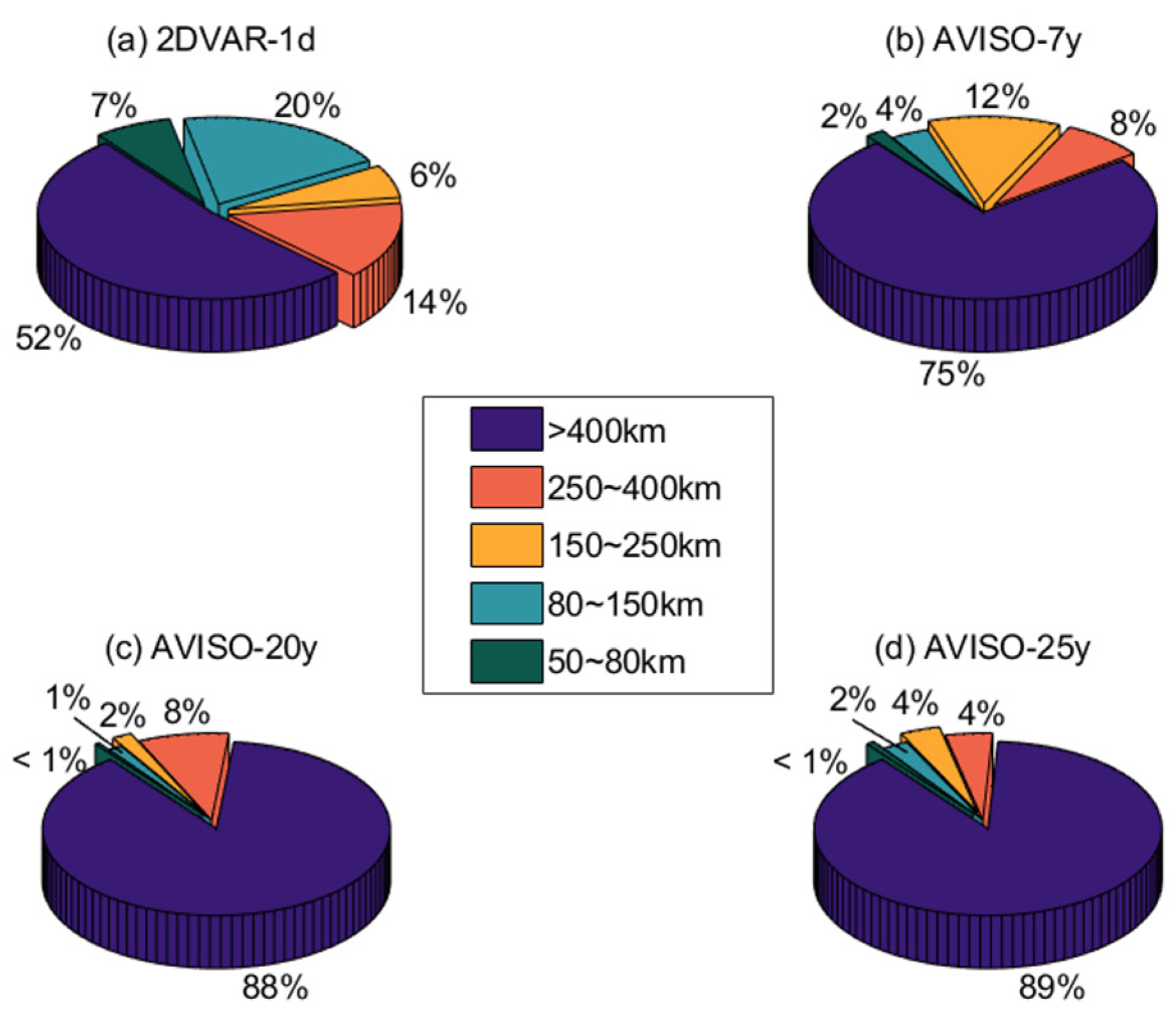
3.1. Signal Proportion of Different Scales in the Background

The 2DVAR method generated the smaller correlation length scale than the AVISO method (Figure 1). For the AVISO method, the correlation length scales increased with time in years averaged for the background. This indicates that, even when a finer spatial grid is used, selecting a too-long averaged period for the background field prevents the reduction in the correlation length scale.

Around the SCS, slightly more than 25% energies of the identified signal in the background errors of the 2DVAR method were for small mesoscale signals (50 km to 150 km), and 20% energies for signals of 150 to 400 km (Figure 2). In the background errors of the AVISO method, small mesoscale (<150 km) signals had a deficient proportion (2–6%) of energies in the 7-, 20-, and 25-year averaged background. Those signals with a spatial scale >400 km accounted for 75% (7 y) and 88% (20 and 25 y) of the total energy, respectively. The 2DVAR method generated more signals that have smaller scales because it uses a day-to-day estimate, giving less weight to low-frequency longer spatial scales, whereas the AVISO methods exhibit the opposite effect at each length scale.

As the length of the background time window increases from day to year, the proportion of energies with large-scale signals remaining in the background errors increased, and the correlation length scale increases. Therefore, using a long-time-averaged background field in the mapping implementation hinders improvement of the resolution capability of the merged maps.

3.2. Evaluation of Accuracy

To validate the reconstruction of small mesoscale structure and consistency with the actual signal, different merged maps were evaluated against independent SST and drifter trajectory data and dependent along-track satellite ADT data. Tides significantly influence the coastal area of the SCS. The continental shelf, at an average depth of 200 m, was not included in the analyses in this section.

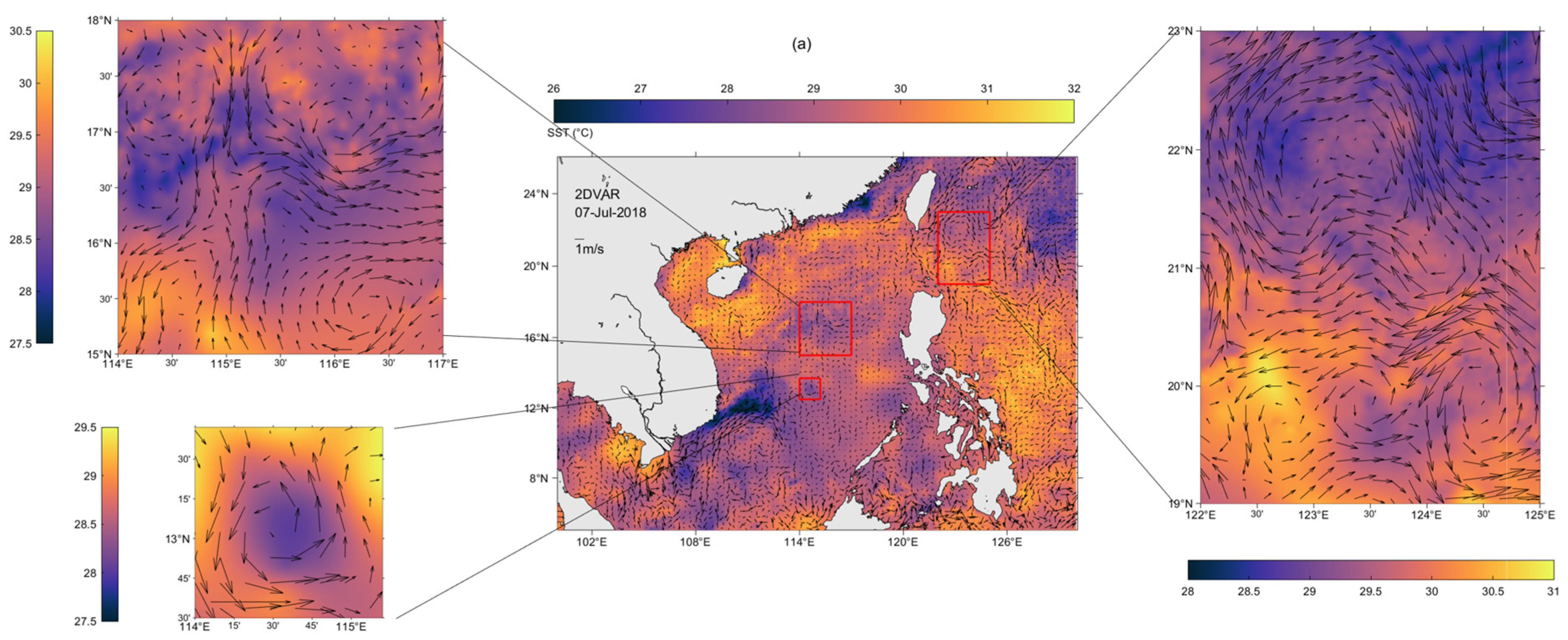
3.2.1. Remote Sensing Evaluation

Although the spatial patterns of anticyclone eddies are not entirely consistent in terms of SST, or are even orthogonal in some weaker eddies [30], SST of mesoscale eddies is often characterized by a warmer center of the anticyclone, similarly, cyclonic eddies often have colder centers. To a certain extent, SST is responsive to small mesoscale dynamic processes in the upper ocean. In this section, we compared the sea surface geostrophic current, inverted from the ADT data, with the MUR SST anomaly (SSTA) to verify the accuracy of the estimated ADT structure [31].

2DVAR single-day surface flow and temperature corresponded highly in terms of refined structural features (Figure 3a). The other three models show this correspondence only at a larger scale, with poor correspondence in terms of the same refined structure (Figure 3b–d). The geostrophic current of the 1/4° AVISO model was weaker than that of the other models. Although the 2DVAR model achieved better reconstruction of mesoscale eddies, it may induce more small-scale noise in the map the same SST.

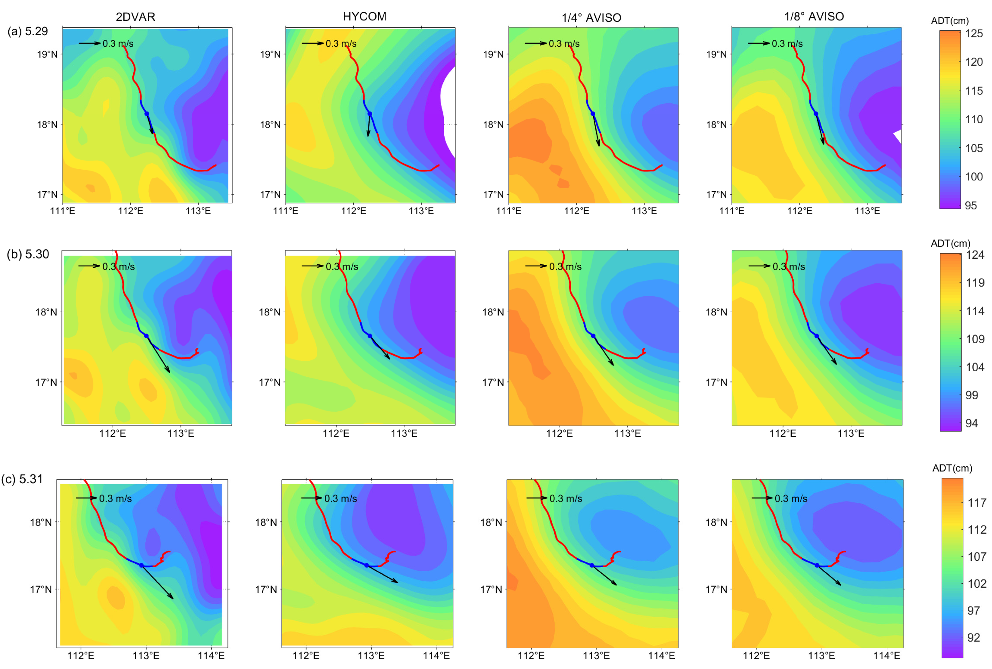
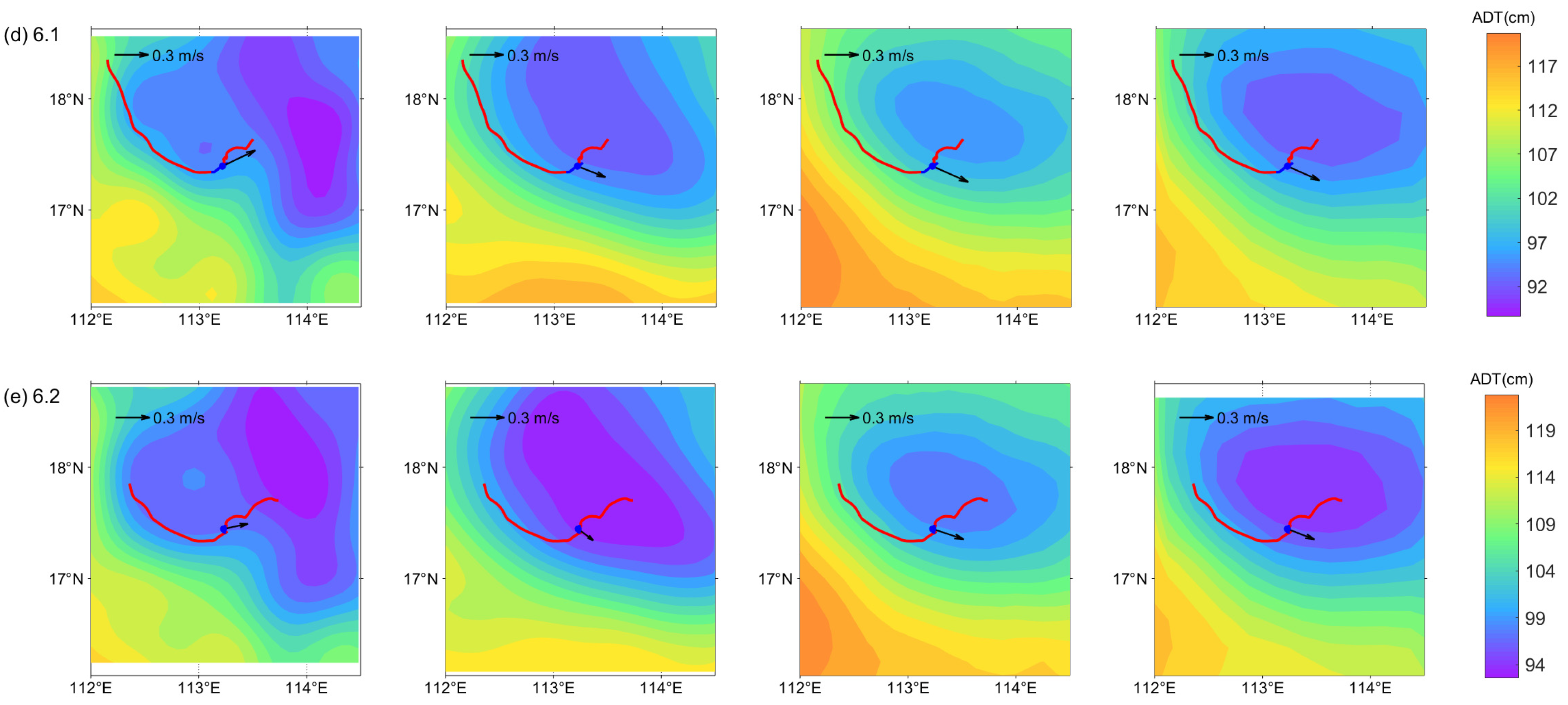
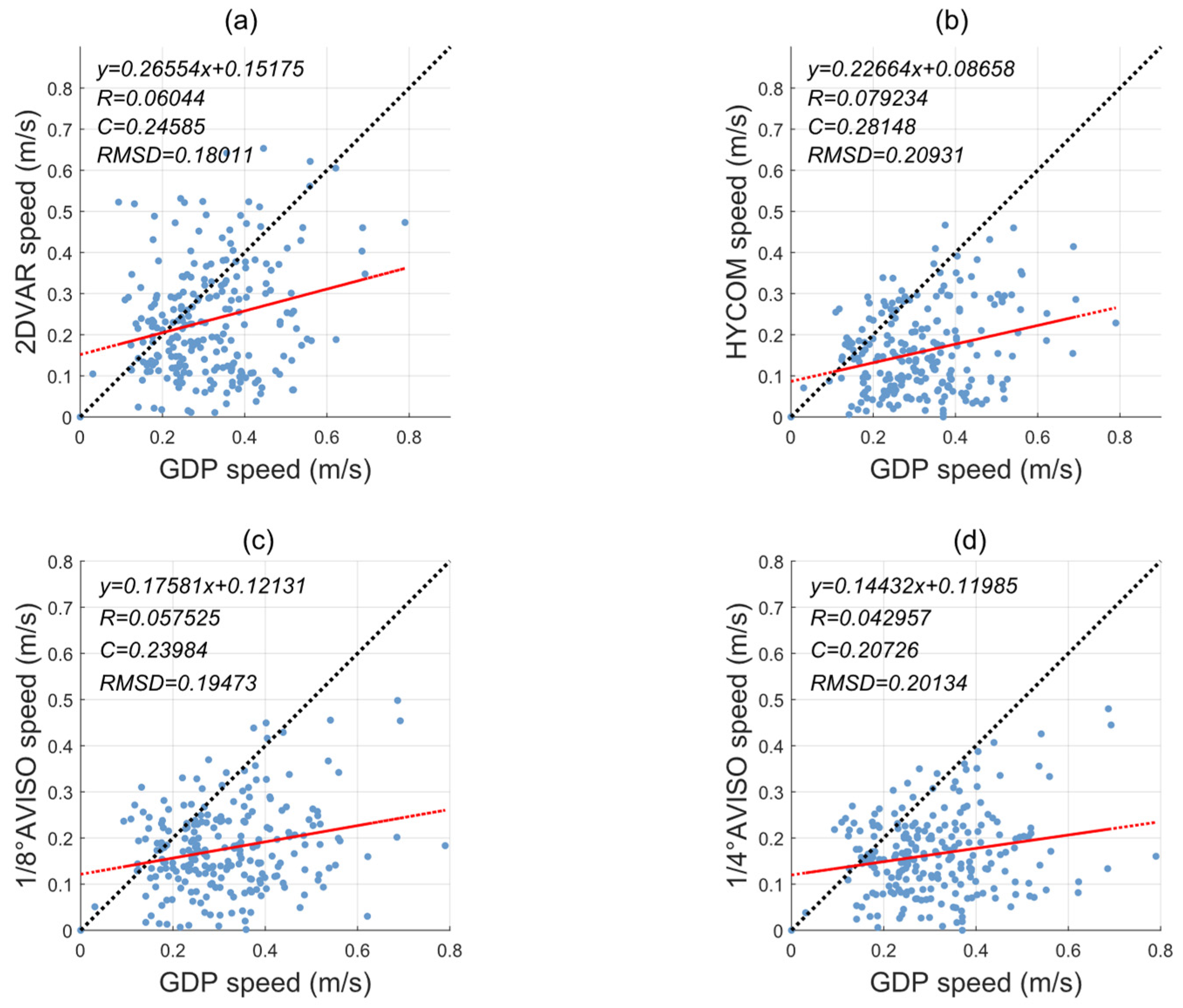
3.2.2. In Situ Evaluation

The in situ GDP hourly drifting buoy datasets [3] is widely used to study small-scale high-frequency dynamic ocean processes. The GDP measures ocean current velocity at a depth of 15 m using a drogue that pulls a surface float underwater with each passing wave. The drogue creates strain against the lower hull of the surface float, thereby reducing the effect of wind. Here, a drifter path in the middle of the SCS, far from the coast areas, was selected to reduce the influence of tides. A drifter with a curved moving path was compared to evaluate its ability to capture the mesoscale structure in the various merged maps.

On 29 May 2018 (Figure 4), the buoy paths were parallel to the contours of the ADT gradients of the four models. On 30 and 31 May 2018 (Figure 4b,c), the buoy paths were almost parallel to the contours of the ADT gradient of the 2DVAR model and perpendicular to those of the other maps. The result of the other models are mostly inconsistent with the buoy data shown in Figure 4d, for 1 June 2018. The relationship between the buoy path and the height field gradient is similar to that in panels c–e of Figure 4. Comparing the 2DVAR height field with that of the stand-alone buoy reveals that the buoy rotated counterclockwise around a small eddy with a low center at SSH, consistent with the eddy characteristics obtained using the 2DVAR method. The two AVISO models and HYCOM have poor reconstructions of smaller-scale eddies, thus resulting in buoy trajectory crossovers with their height fields. Therefore, 2DVAR exhibits certain advantages over the other models in terms of its ability to present smaller mesoscale eddies in the ocean.

All of the models exhibited lower geostrophic velocities than the drifting buoys (Figure 5). Although the HYCOM data were the most concentrated in the regression curve, the 2DVAR regression curve illustrates a better fit, with a slope closest to 1. The 2DVAR model also had the lowest root mean square deviation (RMSD) for the entire map.

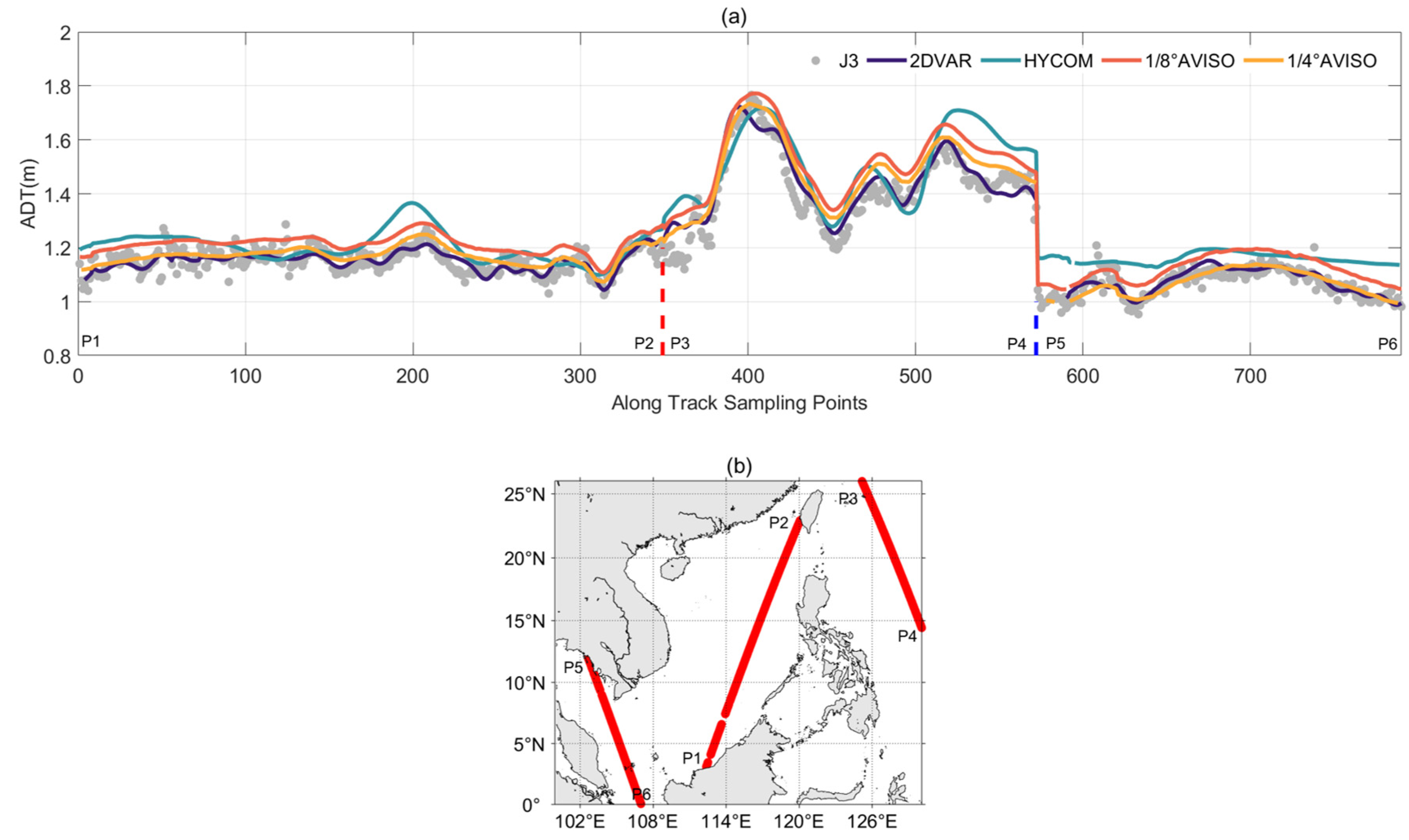
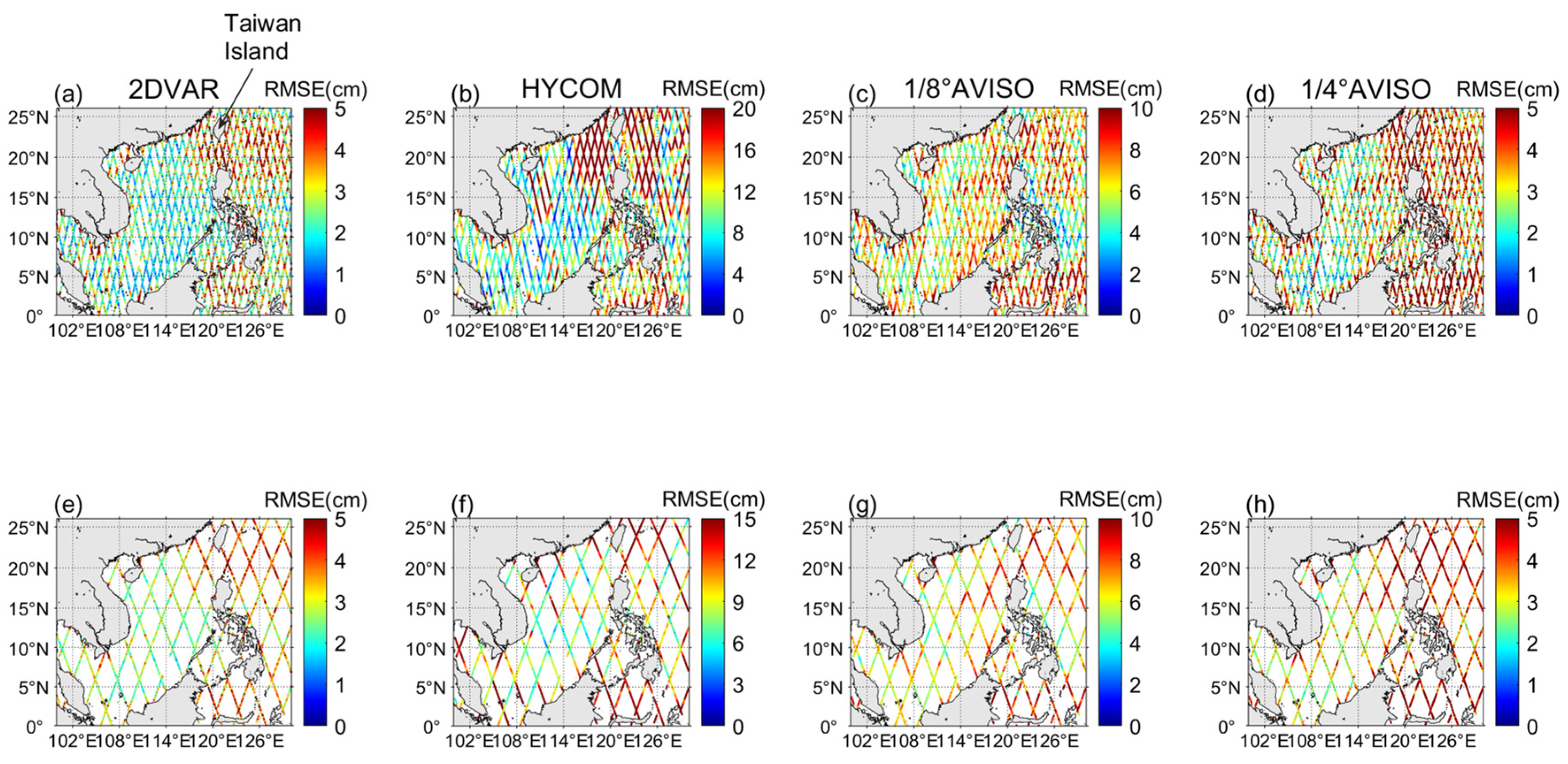
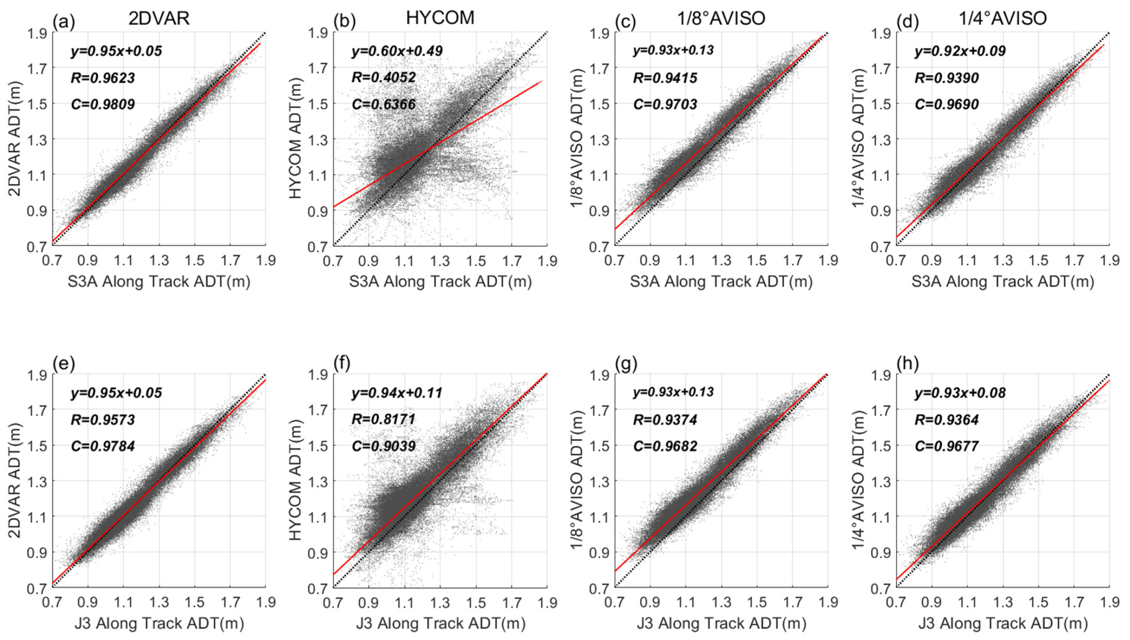
3.2.3. Along-Track Satellite Evaluation

To calculate the root mean square error (RMSE), correlations, and linear regressions of the merged maps and thus evaluate their accuracy, the L3 along-track data from the S3A and J3 satellites were used as the hypothetical true values [11]. S3A has smaller orbital spacing and higher data density satellite than J3, allowing it to cover a larger area in the full-field mapping of RMSE. To illustrate the relationship between the 2DVAR maps and those generated using the other models, an index score (S) comparing the deviations of each product was calculated [12]:

$$S=1-{\sigma }_{2\mathrm{D}\mathrm{V}\mathrm{A}\mathrm{R}}^2/{\sigma }_{\mathrm{O}\mathrm{t}\mathrm{h}\mathrm{e}\mathrm{r}\mathrm{s}}^2$$

(7)

where $\sigma$ is the mean square error for each model; ‘Others’ refers to the models other than 2DVAR; and S is the degree of deviation of other models relative to 2DVAR. A positive S indicates a higher error relative to that of 2DVAR, while a negative S reflects an error less than that of 2DVAR.

Table 2. The accuracy of 4 models. The root mean square error (RMSE, in cm) for entire map compared with along-track S3A and J3 satellite L3 data, and the mean error index score S for entire map of each product compared with 2DVAR.

Experiments/ Models	RMSE [cm]		S
	S3A	J3	S3A	J3
2DVAR	0.0299	0.0340	/	/
HYCOM	1.5946	0.5189	0.8987	0.9421
1/8° AVISO	0.0678	0.0688	0.6658	0.7070
1/4° AVISO	0.0396	0.0414	0.1125	0.2313

lists the mean RMSE and S for the entire map, reflecting the accuracy of the merged maps.

2DVAR had the lowest RMSE for the center waters of the SCS (at only 1–2 cm), followed by the 1/4° AVISO model (at ca. 1 cm higher) (Figure 6a,c,e,g). The 1/8° AVISO model had an RMSE of ca. 5–6 cmca. double those obtained in the previous two models (Figure 6d,h). HYCOM exhibited the highest RMSE (>20 cm, relative to the S3A data) in the northern SCS (Figure 6b) and <10 cm relative to the J3 data (Figure 6f). The large RMSE obtained for the Pacific Ocean, Luzon Strait, and the Celebes Sea was due to the tidal influences in coastal areas and high eddy kinetic energy (EKE) transport from the Pacific crossing Luzon Strait to Kuroshio [32]. In summary, the mean RMSE for the entire map (Table 2) was lowest for the 2DVAR model, at ca. 0.01 cm lower than that of the AVISO global 1/4° model, and substantially lower than that of the HYCOM model. S varied in the same way as RMSE, being highest for HYCOM and lowest for 1/4° AVISO model.

Due to the strong influence of the Kuroshio, the zonal flow in the surface (shallower than 500 m) of the Luzon Strait is typically westward [32]. Thus, most of the high-frequency mesoscale eddies generated from the Bashi and Northern Philippines Strait were propagated from the longest channel of eddy propagation in the SCS to the southwest of the northern SCS (from the Luzon Strait to ca. 18°N, 112°E), often with a long lifecycle [33]. The high RMSE values southwest of Taiwan island in both of the AVISO models reflect the same distribution characteristic as the longest channel of eddy propagation. This result may occur because the increased presence of eddies in the channel increases the spatiotemporal variability in sea surface conditions, increasing the difficulty in reproducing smaller eddies. For the two AVISO maps, the poor scale-recognition resolution resulted in higher RMSE values in the channel. While 2DVAR model benefits from its good scale-recognition resolution, its RMSE exhibited very low consistency with the propagation channel.

The 2DVAR model exhibited a linear regression correlation coefficient (R) > 0.95 and had the highest correlation coefficient (C) (ca. 0.98) (Figure 7a,e). The correlation between the HYCOM data and the S3A hypothesized true value was only 0.64 (Figure 7b), almost 0.30 points smaller than that of the other three models. This is highly consistent with the differences in RMSE values.

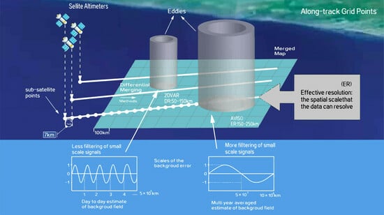
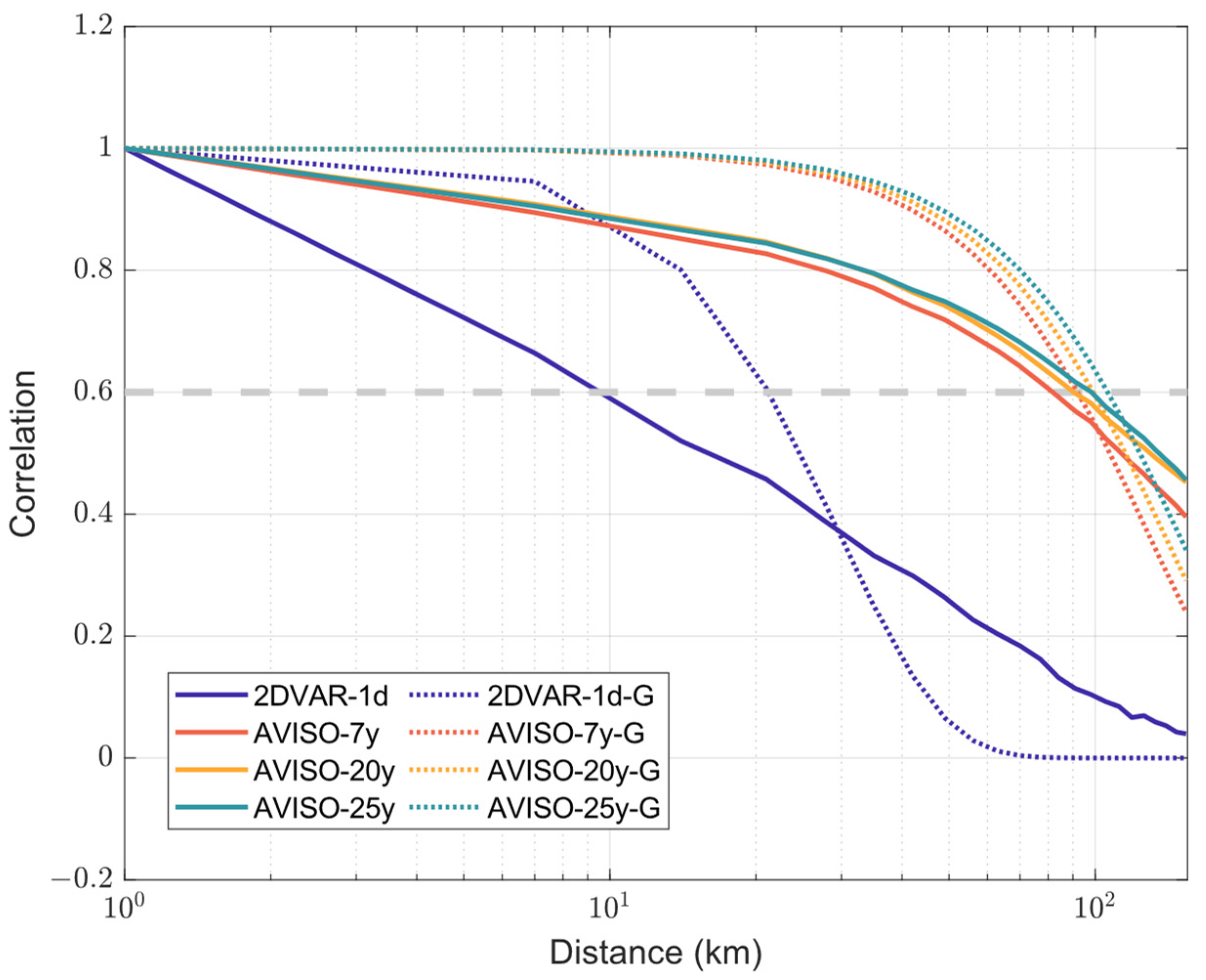
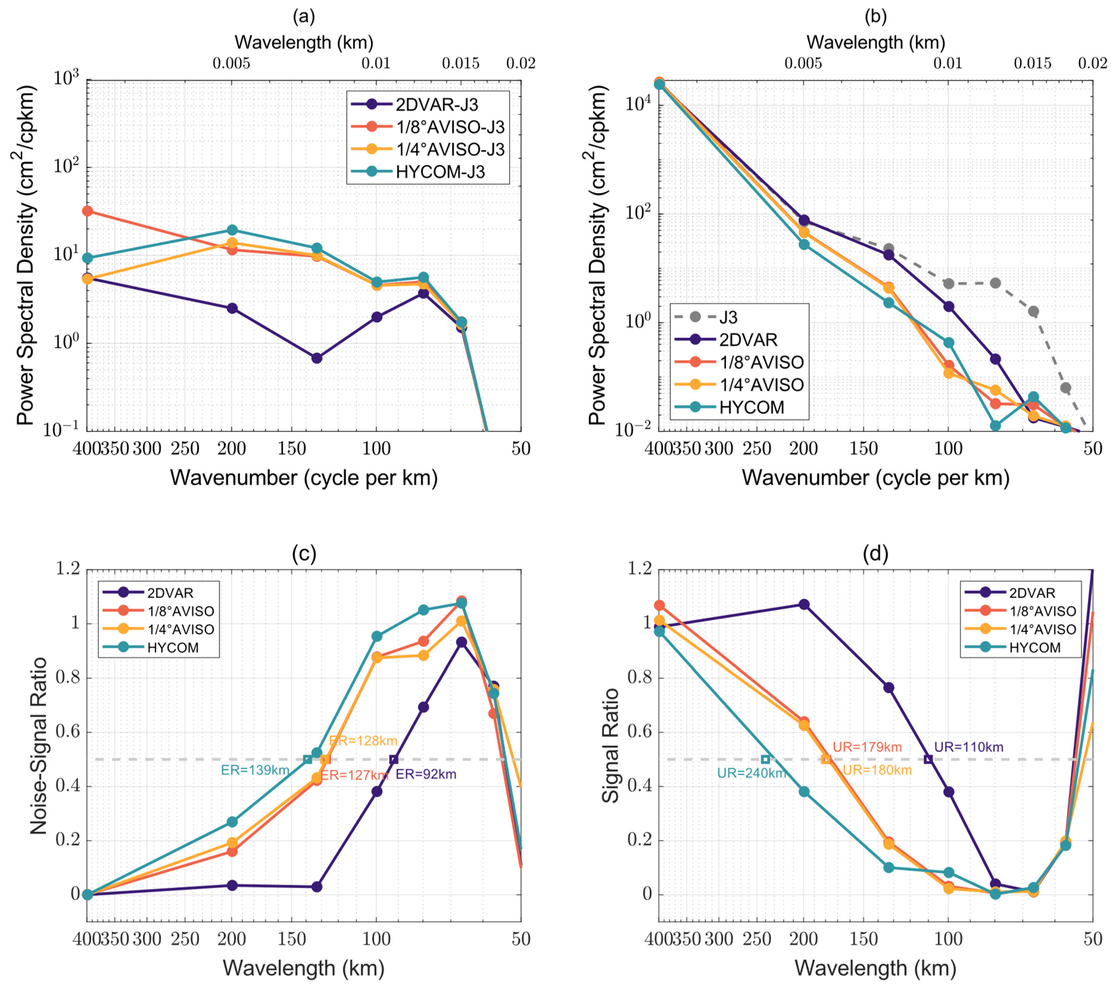
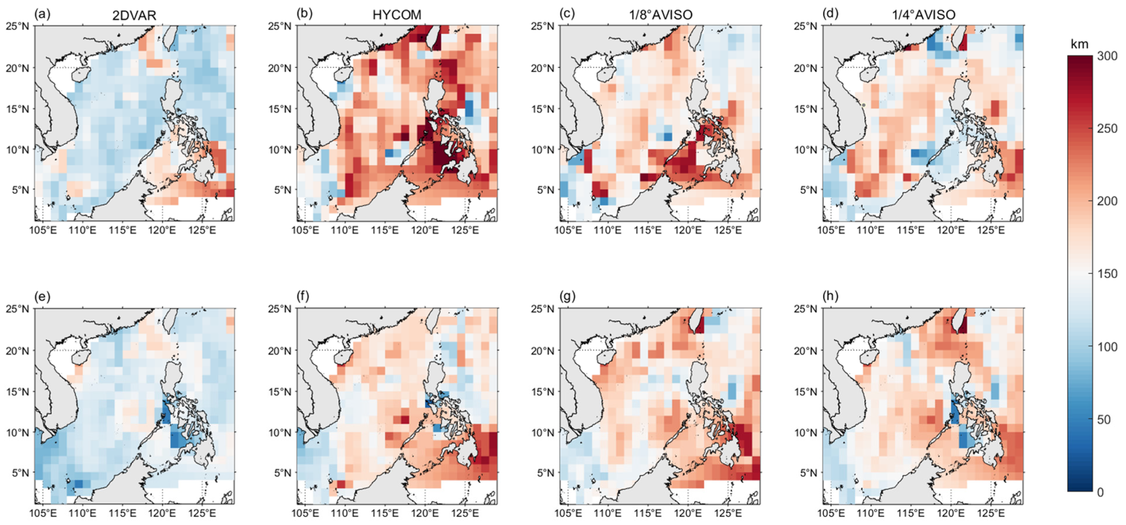
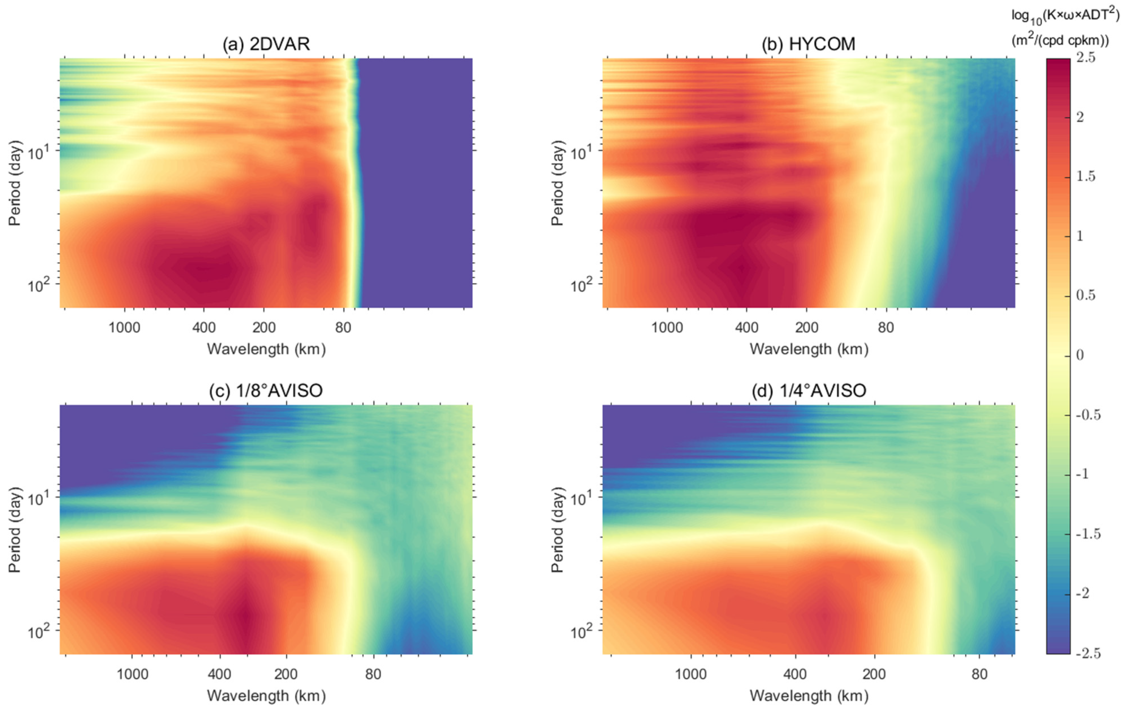
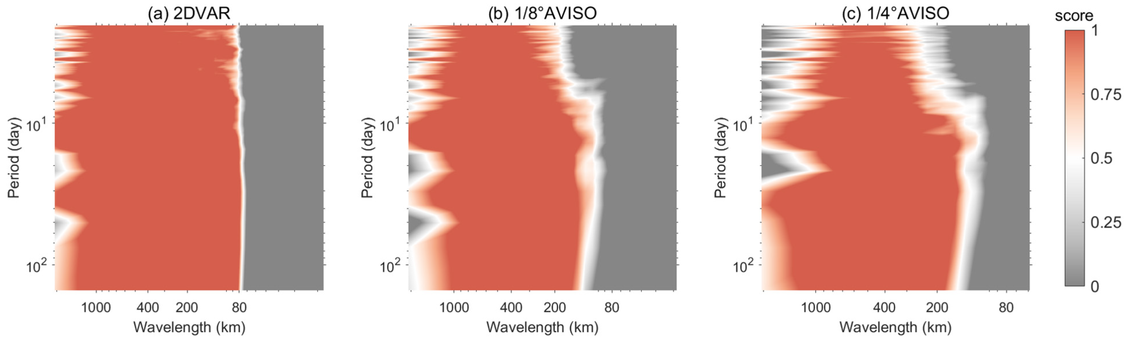
3.3. Evaluation of Effective Resolution

Figure 8a presents the ADT sequence of the along-track sampling points from the four merged maps and J3 satellite data for a randomly selected date (9 July 2018). The track (Figure 8b) is sorted in the sequence P1–6. Among the four merged maps, 2DVAR exhibited the best fit and best reflected the satellite signal amplitude and small-scale information, especially at P1–2. HYCOM performed the worst, with the largest deviation from satellite data, especially at P5–6. The 1/4° AVISO model deviated slightly from the satellite data. The deviation between the 1/8° AVISO and 1/4° AVISO data waveform was almost regular at every sampling point. An offset occurred because the time scale of correlation and the MDT of the customized 1/8° AVISO product had been adjusted.

Each product was a mapping of multiple satellite data, including the J3 data. Part of the merged data approximately 370 and 420 points did not match the ADT variance in J3. The reasons may not only be related to the smaller temporal scales of these processes than that used in 2DVAR or AVISO but also to their smaller spatial scales than the background error correlation coefficient scales.

ER refers to scale-recognition resolution, a parameter that relates the recognition capability of the altimeter product to the dynamic signal of ocean eddies. Scale-recognition resolution is defined as the minimum resolvable spatial scale of the signal in the merged map, and its value indicates the smallest sea-surface eddy that can be distinguished in the signal from the perspective of energy spectral density [13].

Scale-recognition resolution was calculated using the definitions of ER and UR [21] based on the wavenumber PSD of the ADT field, using the observational ADT data as a spatial sequence with distance as the independent variable. ER was obtained using the ratio of the PSD of the noise to the signal, i.e., the noise–signal ratio (NSR). UR was obtained using the ratio of the PSD between the estimated value of the merged maps and the satellite along-track signal, i.e., the signal ratio (SR). At NSR or SR of 0.5, the wavelengths (λ) corresponding to their positions are ER and UR, respectively. By comparing local phase differences, using ER reduces the large systematic error generated by the comparison between the different phases, although it may be more affected by noise. UR reflects a comparison of spatial sequence spectral amplitudes that relatively better represent the energy magnitude of the signal available within the product data. The average value of each grid point along the track during the study period was recorded to obtain the resolution along the track.

Data for the same day as in Figure 8 (9 July 2018) was selected to display the PSD and scale-recognition resolution results. In the wavelength range of 90–400 km, the PSD value of the mapping field deviation of the 2DVAR product was much lower than that of the 1/8° and 1/4° AVISO and HYCOM models (Figure 9a). The PSD value approximately 70–200 km wavelength of the mapping field of the 2DVAR product was higher than that of the other models shown in Figure 9b. Excluding the 2DVAR model, the other three models did not differ substantially in PSD. The order of ER and UR of the same product is consistent among all products (Figure 9c,d). Relative to the two AVISO models, the 2DVAR model had ER and UR values ca. 30% lower, whereas HYCOM had slightly higher ER and UR values.

Both ER and UR of the 2DVAR model were mostly between 50 and 150 km, with the higher resolutions near the coast or islands (Figure 10a–d). The HYCOM data ER showed an extremely high value, (>200 km) and occupying a large area, with the UR mostly between 100 and 200 km (Figure 10b,f). For the two AVISO models, ER showed 150–250 km in a large area, with some being ≥250 km. For the two AVISO models, UR was concentrated approximately 200 km in most parts of the study area. For all four models, ER was much higher in the vicinity of the Philippine Islands and their coastal waters than else. Owing to the presence of anomalously fluctuating signals (noise), which could be confused with small-scale signals in the ocean, ER had limited usefulness for resolving eddies.

By definition, the ER value of an area with a high error increases correspondingly, and the minimum resolved scale of the ocean eddy signal in the data increases. Comparing the error statistics described in Section 3.2.3, ER > UR for most of the regions with large RMSE. For example, for the southwestern waters regions with high EKE, around the Dongsha Islands of Taiwan Island [16], ER < UR for the 1/4°AVISO model, while for the other three models, ER > UR. Based on these findings, for zones with large RMSE values, UR is more effective than ER for identifying eddies.

Determining the ability to reconstruct eddies involves evaluating the scale of the spatial field and the time scale. Based on a previous work [20], we used the time-frequency domain and spatial wavenumber as reference elements to determine the 2D distribution of the energy spectrum of the height field. The merged maps were decomposed via a 3D Fourier transform. In terms of the period, 2DVAR captured the signals much better than the two AVISO models, within 20 d and 80–200 km (Figure 11a,c,d). The frequency wavelength PSD of HYCOM was large in the wavelength range of 200–1000 km and in the period 0–100 d (Figure 11b). The 2DVAR model exhibited a very low proportion of energy for spatial scale of <80 km (Figure 11a) relative to that in the 80–200 km range, owing to filtering by its variational merging. Although the AVISO models had an energy proportion below 80 km (Figure 11c,d), the method filtered out more energy at the 80–200 scale.

The 2DVAR and AVISO models were used as the hypothetical ground truthing to examine the HYCOM data, and a parameter similar to ER was used to score the frequency wavelength PSD (FWPSDs), as follows [20]:

$$FWPSDs=1-FWPSD(ADT-{ADT}_{true})/FWPSD\left({ADT}_{true}\right)$$

(8)

A PSD distribution with a score > 0.5 is considered accurate and reliable. For the 2DVAR models, the HYCOM data were reliable in time–space frequency domain > 80 km, regardless of the time span (Figure 12a). For the two AVISO models, HYCOM was considered reliable only for frequency domains > 150 km, and improved as the time scale increased (Figure 12b,c).

Based on these results, the 2DVAR merged maps have the highest quality and lowest ER among the four models. In an early study [20], 2DVAR merged maps had a higher ER than the 1/4° AVISO merged maps for the East China Sea region, especially in the open ocean and to the north of Taiwan Island, where mesoscale eddies are relatively large and long-lasting. Here, for the SCS, 2DVAR merged maps achieved better performance than 1/4° AVISO merged maps in reconstructing mesoscale oceanic structure, and their ER was as low as 130 km, or even 110 km around the middle latitudes [12]. For the California Current system, the 2DVAR merged maps could resolve smaller scales than the global 1/4° DUACS-DT2018 maps [11]. These findings together demonstrate that the 2DVAR model has advantages in terms of its merged map quality and ER, and without region-dependent.

4. Discussion

4.1. Signal Composition in Background Field and Associated Error

For the AVISO models, the background-field MDT was obtained using a multiyear-averaged SSH field. Therefore, the signal contained in the background field is strongly time-smoothed, and the error associated with the background field contained more large-scale ocean circulation signals, interannual variation, and seasonal variation. At the same time, the 2DVAR background field did not smooth the signal for any time or region, and induct an evolution error to maintain all signals in the merging processes. Therefore, the background error with the 2DVAR method comprised more small and mesoscale signals than that with the AVISO.

4.2. Filtering Effect of Correlation Coefficient Scale in Variational Method

The wavenumber energy spectral density of the background error and the characteristics of the background error covariance have similar physical (filtering) characteristics.

The filtering characteristics of the PSD associated with the background error decrease with the spatial scale, owing to the localization and intermittence of small-scale systems, and small-scale errors can only represent a certain proportion of the background error. When the spatial scale of the correlation coefficient is larger, the proportion represented by small scale error is less. For authentic ocean signals, when the proportion of the signal energy of a certain scale is lower, the error of that scale is more difficult to correct in the merged maps.

Based on these filtering characteristics, and owing to authentic ocean signals of the AVISO merged maps, it is difficult to distinguish small-scale oceanic structure, due to the larger correlation length scale with the AVISO method.

4.3. The Scale of Effective Resolution Compared with Eddy Radius

The correlation length scale was 10 km for 2DVAR and 100 km for AVISO. The 2DVAR ER was 50–150 km, while that of both AVISO models was 150–250 km.

For the eddies in the SCS, the 2DVAR ER range includes the peak wavelength of the eddy radius Rayleigh distribution, whereas AVISO fails to include the peak wavelength. The 2DVAR merged map can reconstruct mesoscale eddies more accurately than the AVISO maps.

4.4. The Restriction of HYCOM and the Advantages of 2DVAR

HYCOM reanalysis was produced using data assimilation. Altimetry data is first used to estimate temperature and salinity vertical profiles, employing the ISOP (Improved Synthetic Ocean Profiles) algorithm. The estimated temperature and salinity profiles are then assimilated into HYCOM. This assimilation method may limit the impact of altimetry data in the reanalysis:

• There is limited historical sampling data, leading to inaccurate assimilation of height field results.
• Non-steric sea surface heights in the altimeter data cannot be assimilated.
• The set of an assimilation thresholds is defined as the noise level of the satellite altimeter (currently set to 4 cm), which restricts the merging of small-scale information.

It is believed that the long background field time window of AVISO is the key factor causing its resolution to decline. The 2DVAR model has additional technical advantages [23]:

• The matrix deformation avoids inversion of the background error covariance matrix and can be minimized over the entire grid domain, and is therefore suitable for solving high-resolution problems with a large number of grid points.
• The processing methods of the background error covariance matrix and observation error covariance matrix are more flexible than those of the other models; this flexibility is convenient for simplifying and introducing dynamic constraints.
• Using the observation operator H, it is easy to merge the observation data of different properties.

Comparing with HYCOM, 2DVAR does not depend on the above assumptions such as ‘noise level’, directly merges along-track data, and applies the correlation length scale to supplement noise filtering, thereby retaining small and mesoscale signals. Therefore, the obtained 2DVAR merged map provides higher quality reconstructions than the map obtained using HYCOM reanalysis data.

4.5. Limitations and Future Work

Although the ER of 2DVAR product has been effectively improved, many small-scale processes still cannot be resolved due to the temporal and spatial scales. To increase the density of observation and acquire more valid information, 2DAVR introduced the evolutionary error in the observation error (R_s = R_m + R_e, the observation error covariance matrix R_s consists of measurement R_m and evolutionary error covariance matrices R_e) to address the difference between observation time and mapping time [12]. In addition, the wide-swath Surface Water and Ocean Topography (SWOT) mission was launched on 15 December 2022. As a result, the findings of this study can be extended to resolve small-scale features in maps derived using data from new multi-satellite altimeters, including SWOT data [34]. The multi-scale data merging will be tried to improve further the ER of merged maps in the future [35].

5. Conclusions

The analyses have shown that the ER of the 2DVAR mapped altimetry data is approximately 130 km, while it is approximately 250 km for both the 1/8° and 1/4° AVISO mapped data products. The factors for increasing the effective resolution was then examined. Both the 2DVAR and AVISO OI methods were formulated based on optimal estimation theory, and they are equivalent to each other [15]. The differences arise only from their implementation.

It was shown that the differences in the effective resolution result from the difference in the chosen background states and thus the associated background error. In the 2DVAR method, the mapped SSH of the previous day was used as the background state, while a 25 yeas mean used as the background state in the AVISO OI method. Thus, the background error with the 2DVAR method are relatively dominated by meso- and small-scale signals. In contrast, the background error with the AVISO OI method is the anomalies from the 25 year mean, and thus it includes large-scale signals, such as interannual and seasonal variabilities. The large-scale signals leads to a larger correlation length scale. A large correlation length scale imposes stronger filtering effect on the merged maps. Thus, the large correlation length scale is the main reason for a low effective resolution with 1/4° AVISO, even with a finer spatial grid of 1/8° AVISO and 1/12° HYCOM.

References

1. Ubelmann, C.; Dibarboure, G.; Gaultier, L.; Ponte, A.L.S.; Ardhuin, F.; Ballarotta, M.; Faugére, Y. Reconstructing Ocean Surface Current Combining Altimetry and Future Spaceborne Doppler Data. J. Geophys. Res. Ocean. 2021, 126, e2020JC016560. [Google Scholar] [CrossRef]
2. Mulet, S.; Rio, M.; Etienne, H.; Artana, C.; Cancet, M.; Dibarboure, G.; Feng, H.; Husson, R.; Picot, N.; Strub, C.P.A.P. The new CNES-CLS18 global mean dynamic topography. Ocean Sci. 2021, 17, 789. [Google Scholar] [CrossRef]
3. Elipot, S.; Lumpkin, R.; Perez, R.C.; Lilly, J.M.; Early, J.J.; Sykulski, A.M. A global surface drifter data set at hourly resolution. J. Geophys. Res. Ocean. 2016, 121, 2937–2966. [Google Scholar]
4. Abdalla, S.; Kolahchi, A.A.; Ablain, M.; Adusumilli, S.; Bhowmick, S.A.; Alou-Font, E.; Amarouche, L.; Andersen, O.B.; Antich, H.; Aouf, L.; et al. Altimetry for the future: Building on 25 years of progress. Adv. Space Res. 2021, 68, 319–363. [Google Scholar] [CrossRef]
5. Wang, G.; Wu, L.; Mei, W.; Xie, S.P. Ocean currents show global intensification of weak tropical cyclones. Nature 2022, 611, 496–500. [Google Scholar] [CrossRef] [PubMed]
6. Davis, R.; Talley, L.; Roemmich, D.; Owens, B.; Rudnick, D.; Toole, J.; Weller, R.; McPhaden, M.; Barth, J. 100 Years of Progress in Ocean Observing Systems. Meteorol. Monogr. 2018, 59, 1–46. [Google Scholar] [CrossRef]
7. Zilberman, N.; Roemmich, D.; Gille, S.; Gilson, J. Estimating the Velocity and Transport of Western Boundary Current Systems: A Case Study of the East Australian Current near Brisbane. J. Atmos. Ocean. Technol. 2018, 35, 1313–1329. [Google Scholar] [CrossRef]
8. Charney, J.; Flierl, G. Oceanic analogues of large scale atmospheric motions. In Evolution of Physical Oceanoaraphy; Warren, B., Wunsch, C., Eds.; MIT Press: Cambridge, MA, USA, 1981; pp. 502–546. [Google Scholar]
9. Yu, H.; Li, J.; Wu, K.; Wang, Z.; Yu, H.; Zhang, S.; Hou, Y.; Kelly, R.M. A global high-resolution ocean wave model improved by assimilating the satellite altimeter significant wave height. Int. J. Appl. Earth Obs. Geoinf. 2018, 70, 43–50. [Google Scholar] [CrossRef]
10. Detlef, S.; Anny, C. Satellite Altimetry Over Oceans and Land Surfaces. Aeronaut. J. 2019, 123, 1297–1298. [Google Scholar] [CrossRef]
11. Archer, M.R.; Li, Z.; Fu, L.L. Increasing the Space–Time Resolution of Mapped Sea Surface Height from Altimetry. J. Geophys. Res. Ocean. 2020, 125, 2019JC015878. [Google Scholar] [CrossRef]
12. Liu, L.; Jiang, X.; Fei, J.; Li, Z. Development and evaluation of a new merged sea surface height product from multi-satellite altimeters. Chin. Sci. Bull. 2020, 65, 1888–1897. [Google Scholar] [CrossRef]
13. Chelton, D.B.; Schlax, M.G.; Samelson, R.M. Global observations of nonlinear mesoscale eddies. Prog. Oceanogr. 2011, 91, 167–216. [Google Scholar] [CrossRef]
14. Chelton, D.; Dibarboure, G.; Pujol, M.I.; Taburet, G.; Schlax, M.G. The Spatial Resolution of AVISO Gridded Sea Surface Height Fields; OSTST: Lake Constance, Germany, 2014; pp. 28–31. Available online: https://meetings.aviso.altimetry.fr/fileadmin/user_upload/tx_ausyclsseminar/files/29Red0900-1_OSTST_Chelton.pdf (accessed on 30 March 2022).
15. Ubelmann, C.; Klein, P.; Fu, L. Dynamic Interpolation of Sea Surface Height and Potential Applications for Future High-Resolution Altimetry Mapping. J. Atmos. Ocean. Technol. 2015, 32, 177–184. [Google Scholar] [CrossRef]
16. Chen, G.; Hou, Y.; Chu, X. Mesoscale eddies in the South China Sea: Mean properties, spatiotemporal variability, and impact on thermohaline structure. J. Geophys. Res. 2011, 116, C06018. [Google Scholar] [CrossRef]
17. Wang, G.; Su, J.; Chu, P.C. Mesoscale eddies in the South China Sea observed with altimeter data. Geophys. Res. Lett. 2003, 30, 2121. [Google Scholar] [CrossRef]
18. Roberts-Jones, J.; Bovis, K.; Martin, M.J.; McLaren, A. Estimating background error covariance parameters and assessing their impact in the OSTIA system. Remote Sens. Environ. 2016, 176, 117–138. [Google Scholar] [CrossRef]
19. Pegliasco, C.; Chaigneau, A.; Morrow, R.; Dumas, F. Detection and tracking of mesoscale eddies in the Mediterranean Sea: A comparison between the Sea Level Anomaly and the Absolute Dynamic Topography fields. Adv. Space Res. 2021, 68, 401–419. [Google Scholar] [CrossRef]
20. Jiang, X.; Liu, L.; Li, Z.; Liu, L.; Sian, K.T.C.L.; Dong, C. A Two-Dimensional Variational Scheme for Merging Multiple Satellite Altimetry Data and Eddy Analysis. Remote Sens. 2022, 14, 3026. [Google Scholar] [CrossRef]
21. Taburet, G.; Pujol, M.; SL-TAC Team. QUID for Sea Level TAC DUACS Products. Available online: https://catalogue.marine.copernicus.eu/documents/QUID/CMEMS-SL-QUID-008-032-068.pdf (accessed on 5 April 2023).
22. Ballarotta, M.; Ubelmann, C.; Pujol, M.I.; Taburet, G.; Fournier, F.; Legeais, J.F.; Faugere, Y.; Delepoulle, A.; Chelton, D.; Dibarboure, G.; et al. On the resolutions of ocean altimetry maps. Ocean Sci. 2019, 15, 1091–1109. [Google Scholar] [CrossRef]
23. Lewis, J.M.; Lakshmivarahan, S.; Maryada, S.K.R. Placement of Observations for Variational Data Assimilation: Application to Burgers’ Equation and Seiche Phenomenon. In Data Assimilation for Atmospheric, Oceanic and Hydrologic Applications; Park, S.K., Xu, L., Eds.; Springer: Cham, Switzerland, 2021; Volume IV, pp. 259–275. [Google Scholar] [CrossRef]
24. JPL MUR MEaSUREs Project. GHRSST Level 4 MUR Global Foundation Sea Surface Temperature Analysis, Version 4.1; PO.DAAC: Pasadena, CA, USA, 2015. [Google Scholar] [CrossRef]
25. Lumpkin, R.; Centurioni, L. Global Drifter Program Quality-Controlled 6-Hour Interpolated Data from Ocean Surface Drifting Buoys. NOAA National Centers for Environmental Information. Dataset. 2019. Available online: https://www.aoml.noaa.gov/phod/gdp/ (accessed on 30 March 2022).
26. Pujol, M.; Egrave, F.; Re, Y.; Taburet, G.; Dupuy, S.E.; Phanie; Pelloquin, C.; Ablain, M.; Picot, N. DUACS DT2014: The new multi-mission altimeter data set reprocessed over 20 years. Ocean Sci. 2016, 12, 1067–1090. [Google Scholar] [CrossRef]
27. Gaspari, G.; Cohn, S.E. Construction of correlation functions in two and three dimensions. Q. J. R. Meteorol. Soc. 1999, 125, 723–757. [Google Scholar] [CrossRef]
28. Li, Z.; Cheng, X.; Gustafson, W.I., Jr.; Vogelmann, A.M. Spectral characteristics of background error covariance and multiscale data assimilation. Int. J. Numer. Methods Fluids 2016, 82, 1035–1048. [Google Scholar] [CrossRef]
29. Daley, R. Atmospheric data assimilation. In Cambridge Atmospheric and Space Science Series; Cambridge University Press: Cambridge, UK, 1991. [Google Scholar]
30. Gaube, P.; Chelton, D.B.; Samelson, R.M.; Schlax, M.G.; O’Neill, L.W. Satellite Observations of mesoscale Eddy-Induced Ekman Pumping. J. Phys. Oceanogr. 2015, 45, 104–132. [Google Scholar] [CrossRef]
31. Hausmann, U.; Czaja, A. The observed signature of mesoscale eddies in sea surface temperature and the associated heat transport. Deep. Sea Res. Part I Oceanogr. Res. Pap. 2012, 70, 60–72. [Google Scholar] [CrossRef]
32. Zhang, Z.; Zhao, W.; Tian, J.; Yang, Q.; Qu, T. Spatial structure and temporal variability of the zonal flow in the Luzon Strait (Article). J. Geophys. Res. Ocean. 2015, 120, 759–776. [Google Scholar] [CrossRef]
33. Liu, Y.; Tian, F.; Chen, G. Statistical characterization of sea surface temperature over mesoscale eddies in the south China sea. Period. Ocean. Univ. China 2020, 50, 146–156. [Google Scholar] [CrossRef]
34. Morrow, R.; Fu, L.; Ardhuin, F.; Benkiran, M.; Chapron, B.; Cosme, E.; D’Ovidio, F.; Farrar, J.T.; Gille, S.; Lapeyre, G.; et al. Global Observations of Fine-Scale Ocean Surface Topography with the Surface Water and Ocean Topography (SWOT) Mission. Front. Mar. Sci. 2019, 6, 232. [Google Scholar] [CrossRef]
35. Li, Z.; Wang, J.; Fu, L. An Observing System Simulation Experiment for Ocean State Estimation to Assess the Performance of the SWOT Mission: Part 1—A Twin Experiment. J. Geophys. Res. Ocean. 2019, 124, 4838–4855. [Google Scholar] [CrossRef]
Figure 1. The correlation length scale and its Gaussian-fit distribution of the 2DVAR and AVISO maps with different background time windows.
Remotesensing 15 04275 g001
Figure 2. Proportion of error energy at different scales of background errors with the 2DVAR and AVISO methods with different background time average windows.
Remotesensing 15 04275 g002
Figure 3. MUR sea surface temperature (SST) and the inversion of geostrophic current from merged absolute dynamic topography (ADT): (a) 2DVAR, (b) HYCOM, (c) 1/8° AVISO, and (d) 1/4° AVISO on 7 July 2018.
Remotesensing 15 04275 g003aRemotesensing 15 04275 g003b
Figure 4. Absolute dynamic topography (ADT) maps of 2DVAR, HYCOM, 1/8° AVISO, and 1/4° AVISO (sorted by column) with the drifting buoy path. The days are (a) 29 May, (b) 30 May, (c) 31 May, (d) 1 June, and (e) 2 June 2018 (sorted by row, respectively). Blue line: drift path of the buoy on the focal days; red line, drift path during the two days before and after. The arrow indicates the geostrophic vectors from the middle moment of the focal day.
Remotesensing 15 04275 g004aRemotesensing 15 04275 g004b
Figure 5. Geostrophic velocity scatter plot and linear regression curve of (a) 2DVAR, (b) HYCOM, (c) 1/8° AVISO, and (d) 1/4° AVISO with the drifting buoy. The slope of the dotted black dot is 1. Equation y on the upper left corner represents linear regression curve which is the dotted line colored in red. R is the correlation of linear regression coefficients. C is the correlation coefficient between the merged map and the drifting buoy data, and the root mean square deviation (RMSD) between the merged map and the drifting buoy data.
Remotesensing 15 04275 g005
Figure 6. Root mean square error (RMSE) on the satellite track of merged absolute dynamic topography (ADT) compared with S3A (ad) and J3 (eh) satellite along-track data: (a,e) 2DVAR, (b,f) HYCOM, (c,g) 1/8° AVISO, and (d,h) 1/4° AVISO. Note that the color scale for each map is differ from each other for the uniform of colors.
Remotesensing 15 04275 g006
Figure 7. Correlations between the merged maps: (a,e) 2DVAR, (b) HYCOM, (c) 1/8° AVISO, (d) 1/4° AVISO, and S3A (ad) and J3 (eh) satellite along-track data. The ratio of the black dotted line is 1; C is the coefficient of correlation; the red dotted line is the linear regression curve; y represents its equation; and R is the coefficient of correlation for linear regression.
Remotesensing 15 04275 g007
Figure 8. The absolute dynamic topography (ADT) sequence (a) from merged maps along the along-track points of satellite J3 on 9 July. The red and blue dashed lines are the separation position between different tracks. The J3 satellite track in the South China Sea (SCS) for 9 July (b); red dotted line). The sequence P1–6 indicates the direction of movement of different parts of the satellite tracks and corresponds to the sequence of the sampling fragments separated by the red and blue dashed lines.
Remotesensing 15 04275 g008
Figure 9. The power spectral density (PSD) that calculated by (a) subtraction and (b) non-subtraction of the J3 data (except for the gray line in (a), it was the origin data of J3 satellite) from the four merged maps (2DVAR, HYCOM, 1/8° AVISO, and 1/4°AVISO). (c) Effective resolution (ER) and (d) useful resolution (UR) of the four merged maps based on NSR and ER, respectively on 9 July.
Remotesensing 15 04275 g009
Figure 10. (ad) Effective resolution (ER) and (eh) useful resolution UR of the four merged models of (a,e) 2DVAR, (b,f) HYCOM, (c,g) 1/8° AVISO, and (d,h) 1/4°AVISO in the South China Sea (SCS) and nearby waters used S3A satellite data as true values; the darker the color is, the larger the ER or UR value is.
Remotesensing 15 04275 g010
Figure 11. The frequency wavelength power spectral density (PSD) values of the four merged maps. Due to the different spatial map resolutions, the coordinate range of each spectrum was different.
Remotesensing 15 04275 g011
Figure 12. The frequency wavelength power spectral density (PSD) values of the three merged maps.
Remotesensing 15 04275 g012