
Geoid Studies in Two Test Areas in Greece Using Different Geopotential Models towards the Estimation of a Reference Geopotential Value

 , , , and
Abstract
:
1. Introduction
2. Materials and Methods
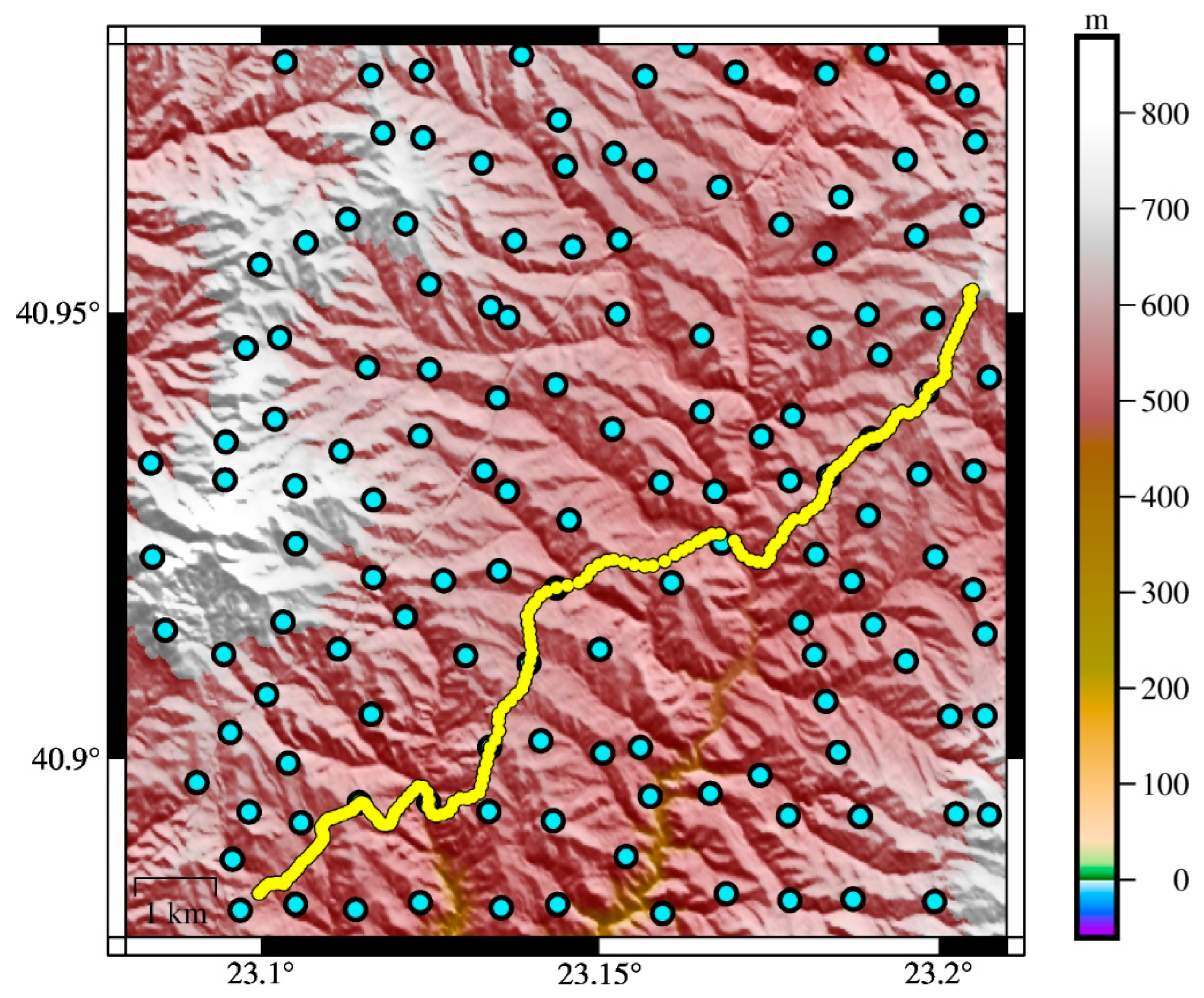
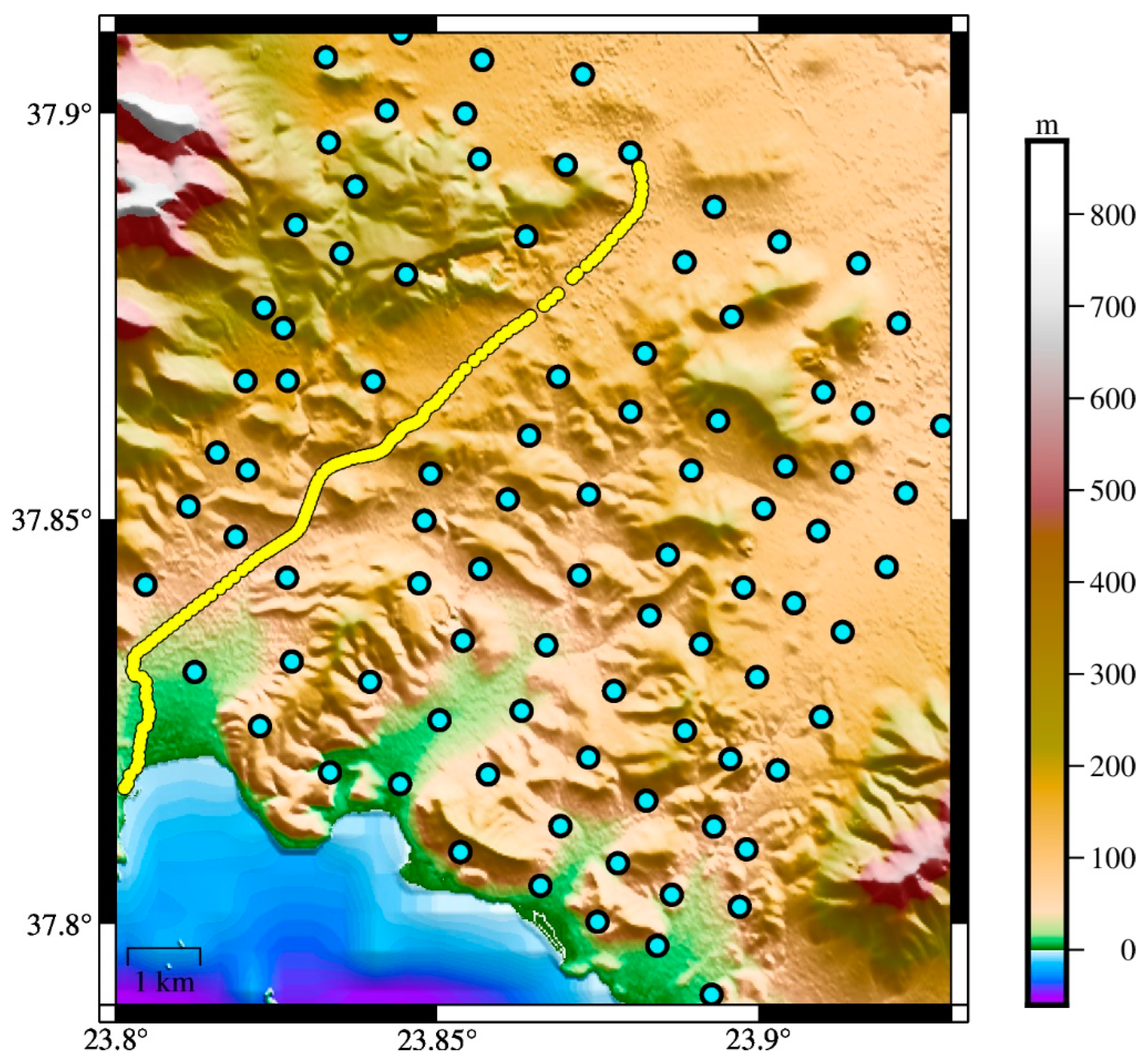
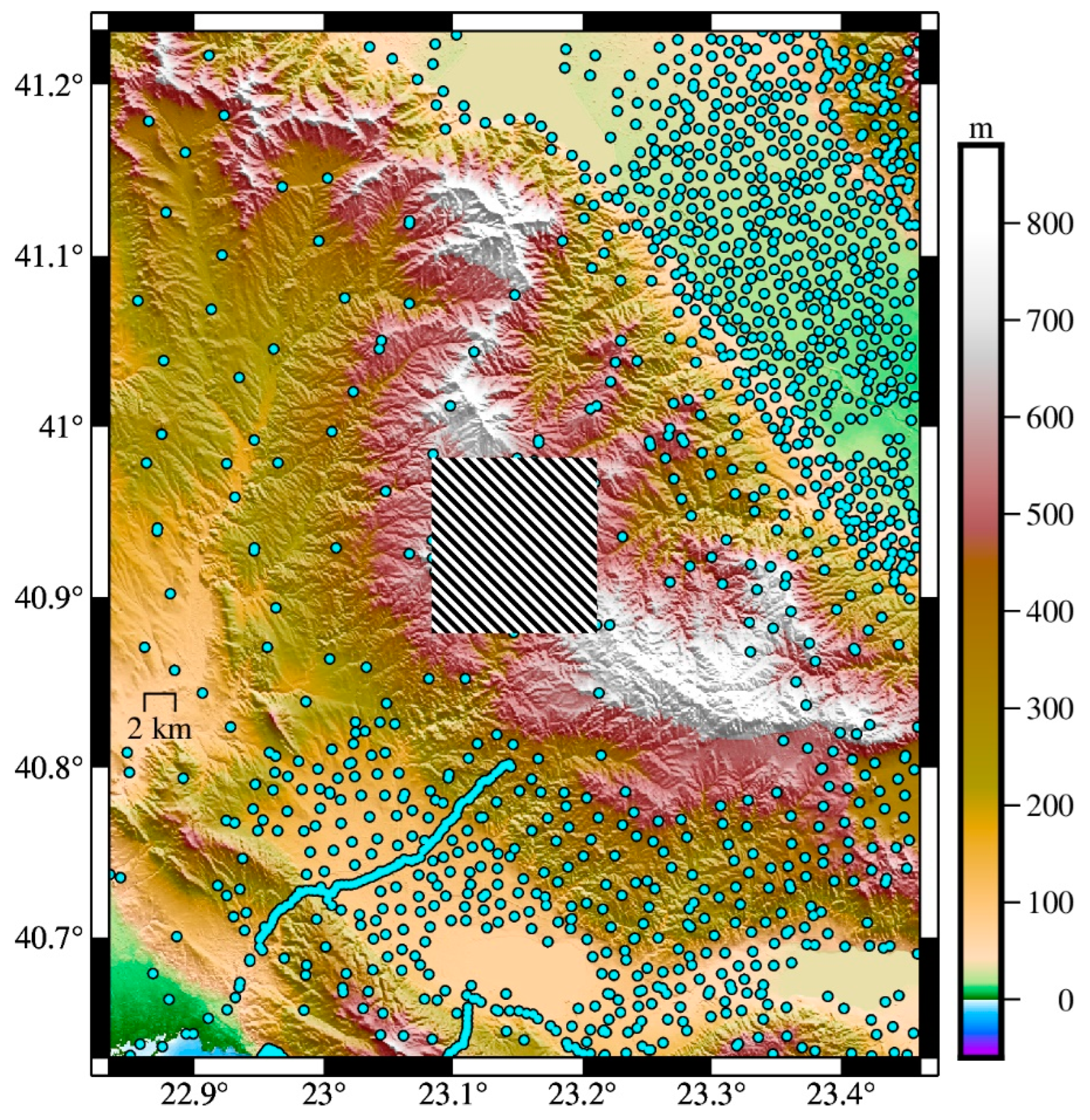
2.1. Available Data
2.1.1. Geopotential Models
2.1.2. Digital Elevation and Bathymetry Model
2.1.3. Gravity, GNSS, and Leveling Data
2.2. Methodology
3. Results
3.1. Gravity Field Modeling
3.2. Geoid Modeling
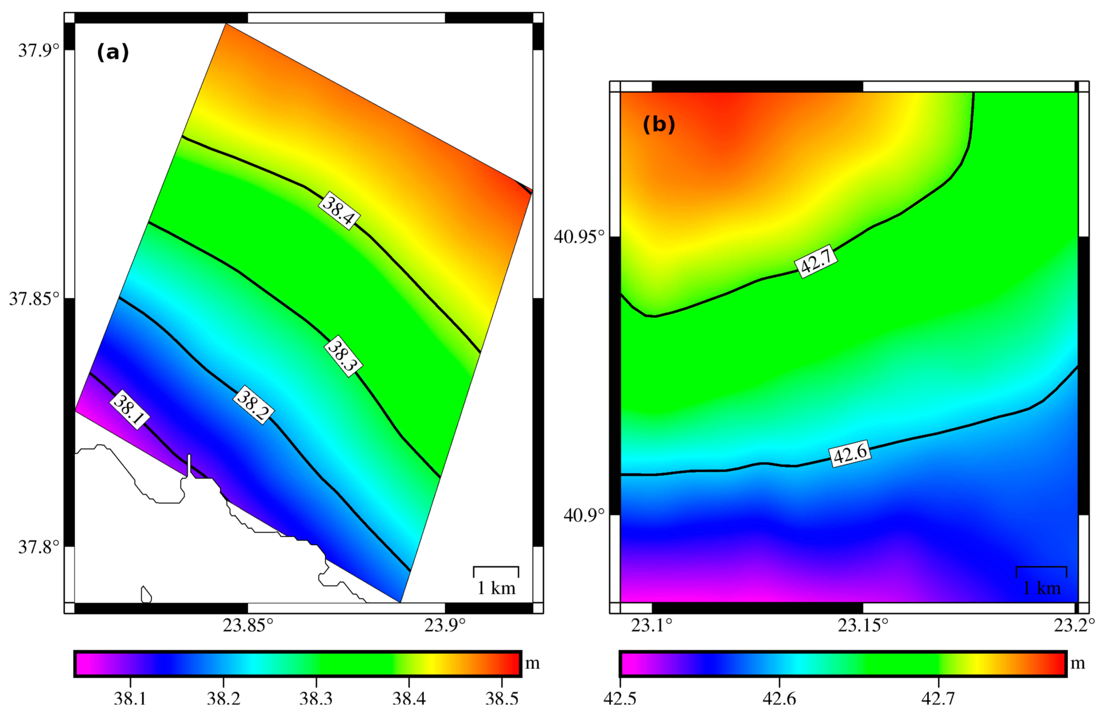
3.3. Reference Geopotential Value
4. Discussion and Conclusions
Author Contributions
Funding
Data Availability Statement
Acknowledgments
Conflicts of Interest
References and Note
- Ihde, J.; Sánchez, L.; Barzaghi, R.; Drewes, H.; Foerste, C.; Gruber, T.; Liebsch, G.; Marti, U.; Pail, R.; Sideris, M. Definition and proposed realization of the International Height Reference System (IHRS). Surv. Geophys. 2017, 38, 549–570. [Google Scholar] [CrossRef]
- Sanchez, L.; Čunderlík, R.; Dayoub, N.; Mikula, K.; Minarechová, Z.; Šíma, Z.; Vatrt, V.; Vojtíšková, M. A conventional value for the geoid reference potential W0. J. Geod. 2016, 90, 815–835. [Google Scholar] [CrossRef]
- Andritsanos, V.D.; Grigoriadis, V.N.; Natsiopoulos, D.A.; Vergos, G.S.; Gruber, T.; Fecher, T. GOCE Variance and Covariance Contribution to Height System Unification. In International Symposium on Gravity, Geoid and Height Systems 2016; Vergos, G., Pail, R., Barzaghi, R., Eds.; Springer: Cham, Switzerland, 2017; Volume 148, pp. 157–164. [Google Scholar] [CrossRef]
- Grigoriadis, V.N.; Kotsakis, C.; Tziavos, I.N.; Vergos, G.S. Estimation of the geopotential value Wo for the local vertical datum of continental Greece using EGM08 and GPS/leveling data. In Gravity, Geoid and Height Systems; Marti, U., Ed.; Springer: Cham, Switzerland, 2014; Volume 141, pp. 249–255. [Google Scholar] [CrossRef]
- Grigoriadis, V.N.; Lambrou, E.; Vergos, G.S.; Tziavos, I.N. Assessment of the Greek Vertical Datum: A Case Study in Central Greece. In International Symposium on Gravity, Geoid and Height Systems 2016; Vergos, G., Pail, R., Barzaghi, R., Eds.; Springer: Cham, Switzerland, 2017; Volume 148, pp. 185–191. [Google Scholar] [CrossRef]
- Kotsakis, C.; Katsambalos, K.; Ampatzidis, D. Estimation of the zero-height geopotential level in a local vertical datum from inversion of co-located GPS, leveling and geoid heights: A case study in the Hellenic islands. J. Geod. 2012, 86, 423–439. [Google Scholar] [CrossRef]
- Vergos, G.S.; Erol, B.; Natsiopoulos, D.A.; Grigoriadis, V.D.; Işık, M.S.; Tziavos, I.N. Preliminary results of GOCE-based height system unification between Greece and Turkey over marine and land areas. Acta Geod. Geophys. 2018, 53, 61–79. [Google Scholar] [CrossRef]
- Forsberg, R. A Study of Terrain Reductions, Density Anomalies and Geophysical Inversion Methods in Gravity Field Modelling; Technical Report OSU Report 1984, No 355; Department of Geodetic Science, The Ohio State University: Columbus, OH, USA, 1984. [Google Scholar]
- Rexer, M.; Hirt, C.; Blazej, B.; Holmes, S. Solution to the spectral filter problem of residual terrain modelling (RTM). J. Geod. 2018, 92, 675–690. [Google Scholar] [CrossRef]
- Tapley, B.D.; Bettadpur, S.; Ries, J.C.; Thompson, P.F.; Watkins, M.M. GRACE Measurements of Mass Variability in the Earth System. Science 2004, 305, 503–505. [Google Scholar] [CrossRef] [PubMed]
- Tapley, B.D.; Watkins, M.M.; Flechtner, F.; Reigber, C.; Bettadpur, S.; Rodell, M.; Sasgen, I.; Famiglietti, J.S.; Landerer, F.W.; Chambers, D.P.; et al. Contributions of GRACE to understanding climate change. Nat. Clim. Chang. 2019, 9, 358–369. [Google Scholar] [CrossRef] [PubMed]
- Kornfeld, R.P.; Arnold, B.W.; Gross, M.A.; Dahya, N.T.; Klipstein, W.M.; Gath, P.F.; Bettadpur, S. GRACE-FO: The Gravity Recovery and Climate Experiment Follow-On Mission. J. Spacecr. Rocket. 2019, 56, 931–951. [Google Scholar] [CrossRef]
- Landerer, F.W.; Flechtner, F.M.; Save, H.; Webb, F.H.; Bandikova, T.; Bertiger, W.I.; Bettadpur, S.V.; Byun, S.H.; Dahle, C.; Dobslaw, H.; et al. Extending the global mass change data record: GRACE Follow-On instrument and science data performance. Geophys. Res. Lett. 2020, 47, e2020GL088306. [Google Scholar] [CrossRef]
- Siry, J.W. The LAGEOS System; NASA Technical Report; Washington, DC, USA; TM-X-73072; 1975. Available online: https://ntrs.nasa.gov/api/citations/19760006091/downloads/19760006091.pdf (accessed on 21 May 2021).
- Ibba, R.; Rum, G.; Varesio, F.; Bussolino, L. IRIS-LAGEOS 2 mission. Acta Astronaut. 1989, 19, 521–527. [Google Scholar] [CrossRef]
- Tziavos, I.N.; Vergos, G.S.; Grigoriadis, V.N.; Tzanou, E.A.; Natsiopoulos, D.A. Validation of GOCE/GRACE Satellite Only and Combined Global Geopotential Models over Greece in the Frame of the GOCESeaComb Project. In IAG 150 Years; Rizos, C., Willis, P., Eds.; Springer: Cham, Switzerland, 2015; Volume 143, pp. 297–304. [Google Scholar] [CrossRef]
- Pavlis, N.K.; Holmes, S.A.; Kenyon, S.C.; Factor, J.K. The development and evaluation of the Earth Gravitational Model 2008 (EGM2008). J. Geophys. Res. Solid Earth 2012, 117, B04406. [Google Scholar] [CrossRef]
- Gomez, M.E.; Perdomo, R.; Del Cogliano, D. Validation of recent geopotential models in Tierra Del Fuego. Acta Geophys. 2017, 65, 931–943. [Google Scholar] [CrossRef]
- Förste, C.; Bruinsma, S.; Abrikosov, O.; Flechtner, F.; Marty, J.-C.; Lemoine, J.-M.; Dahle, C.; Neumayer, H.; Barthelmes, F.; König, R.; et al. EIGEN-6C4 The latest combined global gravity field model including GOCE data up to degree and order 2190 of GFZ Potsdam and GRGS Toulouse. In Proceedings of the 5th GOCE User Workshop, Paris, France, 25–28 November 2014. [Google Scholar]
- Gilardoni, M.; Reguzzoni, M.; Sampietro, D. GECO: A global gravity model by locally combining GOCE data and EGM2008. Stud. Geophys. Geod. 2016, 60, 228–247. [Google Scholar] [CrossRef]
- Ries, J.B.; Bettadpur, S.; Eanes, R.; Kang, Z.; Ko, U.; McCullough, C.; Nagel, P.; Pie, N.; Poole, S.; Richter, T.; et al. The Combined Gravity Model GGM05C; GFZ Data Services: Potsdam, Germany, 2016. [Google Scholar] [CrossRef]
- Fecher, T.; Pail, R.; Gruber, T.; Consortium, G. GOCO05c: A new combined gravity field model based on full normal equations and regionally varying weighting. Surv. Geophys. 2017, 38, 571–590. [Google Scholar] [CrossRef]
- Godah, W.; Krynski, J.; Szelachowska, M. The use of absolute gravity data for the validation of Global Geopotential Models and for improving quasigeoid heights determined from satellite-only Global Geopotential Models. J. Appl. Geophys. 2018, 152, 38–47. [Google Scholar] [CrossRef]
- Wu, Y.; He, X.; Luo, Z.; Shi, H. An Assessment of Recently Released High-Degree Global Geopotential Models Based on Heterogeneous Geodetic and Ocean Data. Front. Earth Sci. 2021, 9, 749611. [Google Scholar] [CrossRef]
- Nyoka, C.J.; Md Din, A.H.; Pasuya, M.F.; Omar, A.H. Rigorous evaluation of global geopotential models for geoid modelling: A case study in Kenya. J. Afr. Earth Sci. 2022, 194, 104612. [Google Scholar] [CrossRef]
- Isik, M.S.; Çevikalp, M.R.; Erol, B.; Erol, S. Improvement of GOCE-Based Global Geopotential Models for Gravimetric Geoid Modeling in Turkey. Geosciences 2022, 12, 432. [Google Scholar] [CrossRef]
- Haagmans, R.; de Min, E.; von Gelderen, M. Fast evaluation of convolution integrals on the sphere using 1D FFT, and a com- parison with existing methods for Stokes’ integral. Manuscripta Geod. 1993, 18, 227–241. [Google Scholar]
- Lyszkowicz, A.; Nastula, J.; Zielinski, J.B.; Birylo, M. A New Model of Quasigeoid for the Baltic Sea Area. Remote Sens. 2021, 13, 2580. [Google Scholar] [CrossRef]
- Kvas, A.; Mayer-Gürr, T.; Krauss, S.; Brockmann, J.M.; Schubert, T.; Schuh, W.-D.; Pail, R.; Gruber, T.; Jäggi, A.; Meyer, U. The satellite-only gravity field model GOCO06s. In GFZ Data Services; GFZ: Potsdam, Germany, 2019. [Google Scholar] [CrossRef]
- Kvas, A.; Brockmann, J.M.; Krauss, S.; Schubert, T.; Gruber, T.; Meyer, U.; Mayer-Gürr, T.; Schuh, W.-D.; Jäggi, A.; Pail, R. GOCO06s—A satellite-only global gravity field model. Earth Syst. Sci. Data 2021, 13, 99–118. [Google Scholar] [CrossRef]
- Bruinsma, S.L.; Förste, C.; Abrikosov, O.; Lemoine, J.-M.; Marty, J.-C.; Mulet, S.; Rio, M.-H.; Bonvalot, S. ESA’s satellite-only gravity field model via the direct approach based on all GOCE data. Geophys. Res. Lett. 2014, 41, 7508–7514. [Google Scholar] [CrossRef]
- Brockmann, J.M.; Schubert, T.; Schuh, W.-D. An improved model of the Earth’s static gravity field solely derived from reprocessed GOCE data. Surv. Geophys. 2021, 42, 277–316. [Google Scholar] [CrossRef]
- Zingerle, P.; Brockmann, J.M.; Pail, R.; Gruber, T.; Willberg, M. The polar extended gravity field model TIM_R6e. In GFZ Data Services; GFZ: Potsdam, Germany, 2019. [Google Scholar] [CrossRef]
- Lu, B.; Luo, Z.; Zhong, B.; Zhou, H.; Flechtner, F.; Förste, C.; Barthelmes, F.; Zhou, R. The gravity field model IGGT_R1 based on the second invariant of the GOCE gravitational gradient tensor. J. Geod. 2017, 92, 561–572. [Google Scholar] [CrossRef]
- Mayer-Gürr, T.; Behzadpur, S.; Ellmer, M.; Kvas, A.; Klinger, B.; Strasser, S.; Zehentner, N. ITSG-Grace2018—Monthly, Daily and Static Gravity Field Solutions from GRACE. In GFZ Data Services; GFZ: Potsdam, Germany, 2018. [Google Scholar] [CrossRef]
- Kvas, A.; Behzadpour, S.; Ellmer, M.; Klinger, B.; Strasser, S.; Zehentner, N.; Mayer-Gürr, T. ITSG-Grace2018: Overview and evaluation of a new GRACE-only gravity field time series. J. Geophys. Res. Solid Earth 2019, 124, 9332–9344. [Google Scholar] [CrossRef]
- Liang, W.; Li, J.; Xu, X.; Zhang, S.; Zhao, Y. A High-Resolution Earth’s Gravity Field Model SGG-UGM-2 from GOCE, GRACE, Satellite Altimetry, and EGM2008. Engineering 2020, 6, 860–878. [Google Scholar] [CrossRef]
- Chen, J.; Zhang, X.; Chen, Q.; Shen, Y.; Nie, Y. Static Gravity Field Recovery and Accuracy Analysis Based on Reprocessed GOCE Level 1b Gravity Gradient Observations. In Proceedings of the EGU General Assembly 2022, Vienna, Austria, 23–27 May 2022. EGU22-6771. [Google Scholar] [CrossRef]
- Chen, Q.; Shen, Y.; Francis, O.; Chen, W.; Zhang, X.; Hsu, H. Tongji-Grace02s and Tongji-Grace02k: High-precision static GRACE-only global Earth’s gravity field models derived by refined data processing strategies. J. Geophys. Res. Solid Earth 2018, 123, 6111–6137. [Google Scholar] [CrossRef]
- Zingerle, P.; Pail, R.; Thomas, G.; Oikonomidou, X. The experimental gravity field model XGM2019e. In GFZ Data Services; GFZ: Potsdam, Germany, 2019. [Google Scholar] [CrossRef]
- Zingerle, P.; Pail, R.; Gruber, T.; Oikonomidou, X. The combined global gravity field model XGM2019e. J. Geod. 2020, 94, 64. [Google Scholar] [CrossRef]
- DLR e.V.; Airbus Defense and Space GmbH. Copernicus DEM GLO-30. Provided under COPERNICUS by the European Union and ESA; all rights reserved, 2018.
- Hellenic Navy Hydrographic Service. Digital Terrain Model (DTM) of the Greek Seas. Available online: https://www.hnhs.gr/ (accessed on 24 March 2021).
- Grigoriadis, V.N.; Andritsanos, V.D.; Natsiopoulos, D.A. Validation of Recent DSM/DEM/DBMs in Test Areas in Greece Using Spirit Leveling, GNSS, Gravity and Echo Sounding Measurements. ISPRS Int. J. Geo-Inf. 2023, 12, 99. [Google Scholar] [CrossRef]
- Grigoriadis, V.N.; Andritsanos, V.D.; Natsiopoulos, D. Validation of the Hellenic Gravity Network in the Frame of the ModernGravNet Project. In International Association of Geodesy Symposia; Springer: Berlin/Heidelberg, Germany, 2022. [Google Scholar] [CrossRef]
- Mäkinen, J. The permanent tide and the International Height Reference Frame IHRF. J. Geod. 2021, 95, 106. [Google Scholar] [CrossRef]
- Grigoriadis, V.N. Geodetic and Geophysical Approach of the Earth’s Gravity Field and Applications in the Hellenic Area. Ph.D. Dissertation, Department of Geodesy & Surveying, School of Rural and Surveying Engineering, Aristotle University of Thessaloniki, Thessaloniki, Greece, 2009. (In Greek). [Google Scholar] [CrossRef]
- Heiskanen, W.A.; Moritz, H. Physical Geodesy; W.H. Freeman and Co.: San Francisco, CA, USA, 1967. [Google Scholar]
- Flury, J.; Rummel, R. On the geoid–quasigeoid separation in mountain areas. J. Geod. 2009, 83, 829–847. [Google Scholar] [CrossRef]
- Rapp, R.H. A FORTRAN Program for the Computation of Gravimetric Quantities from High-Degree Spherical Harmonic Expansions; Technical Report OSU Report 1982, No 334; Department of Geodetic Science, The Ohio State University: Columbus, OH, USA, 1982. [Google Scholar]
- Rexer, M.; Hirt, C.; Claessens, S.; Tenzer, R. Layer-based modelling of the Earth’s gravitational potential up to 10km scale in spherical harmonics and ellipsoidal approximation. Surv. Geophys. 2016, 37, 1035–1074. [Google Scholar] [CrossRef]
- Hirt, C.; Kuhn, M.; Claessens, S.; Pail, R.; Seitz, K.; Gruber, T. Study of the Earth’s short scale gravity field using the ERTM2160 gravity model. Comput. Geosci. 2014, 73, 71–80. [Google Scholar] [CrossRef]
- Sansò, F.; Sideris, M.G. (Eds.) Geoid Determination: Theory and Methods; Springer: Berlin/Heidelberg, Germany, 2013; pp. 145–151. [Google Scholar]
- Ekman, M. Impacts of geodynamic phenomena on systems for height and gravity. Bull. Geod. 1989, 63, 281–296. [Google Scholar] [CrossRef]
- Mylona-Kotrogianni, H. The 1st order leveling net of Greece (in Greek). Bull. Hell. Mil. Geogr. Serv. 1990, 50, 1–26. (In Greek) [Google Scholar]


| Model | Max Degree | Source Data | Reference |
|---|---|---|---|
| EGM2008 | 2190 | A, G, S (GRACE) | [17] |
| EIGEN-6C4 | 2190 | A, G, S (GOCE, GRACE, Lageos) | [19] |
| GOCO06S | 300 | S (GOCE, GRACE, etc.) | [29,30] |
| GO CONS GCF 2 DIR R6 | 300 | S (GOCE, GRACE, Lageos) | [31] |
| GO CONS GCF 2 TIM R6 | 300 | S (GOCE) | [32] |
| GO CONS GCF 2 TIM R6e | 300 | G (Polar regions), S (GOCE) | [33] |
| IGGT R1C | 240 | G, S (GOCE, GRACE) | [34] |
| ITSG_GRACE2018S | 200 | S (GRACE) | [35,36] |
| SGG-UGM-2 | 2190 | A, EGM2008, S (GOCE, GRACE) | [37] |
| Tongji-GMMG2021S | 300 | S (GOCE, GRACE) | [38] |
| TongjiGRACE02K | 180 | S (GRACE) | [39] |
| XGM2019 | 760 | A, G, S (GOCO06S) | [40,41] |
| XGM2019e | 5540 | A, G, S (GOCO06S), Τ | |
| XGM2019e_2159 | 2190 | A, G, S (GOCO06S), Τ |
| Northern Area | Central Area | ||||||||||||||
|---|---|---|---|---|---|---|---|---|---|---|---|---|---|---|---|
| d/o | 180 | 200 | 240 | 280 | 300 | 760 | 2190 | 180 | 200 | 240 | 280 | 300 | 760 | 2190 | |
| EGM2008 | mean | 46.44 | 43.44 | 39.11 | 44.39 | 52.22 | 11.12 | −4.09 | 7.93 | 17.49 | 18.31 | 16.96 | 8.59 | −7.72 | −4.01 |
| stdev | 7.76 | 7.63 | 8.38 | 8.05 | 8.51 | 8.06 | 7.16 | 6.04 | 5.78 | 5.49 | 5.98 | 5.99 | 5.58 | 4.38 | |
| range | 38.05 | 37.09 | 38.97 | 37.74 | 37.70 | 36.82 | 32.38 | 30.24 | 29.08 | 27.20 | 28.42 | 28.72 | 28.17 | 24.39 | |
| EIGEN-6C4 | mean | 47.41 | 44.17 | 39.79 | 44.96 | 52.97 | 11.85 | −3.42 | 9.40 | 18.82 | 19.98 | 18.44 | 10.02 | −6.17 | −2.84 |
| stdev | 7.74 | 7.60 | 8.34 | 8.01 | 8.47 | 8.05 | 7.21 | 6.04 | 5.79 | 5.51 | 6.00 | 6.02 | 5.64 | 4.35 | |
| range | 37.81 | 36.85 | 38.75 | 37.56 | 37.53 | 36.68 | 32.66 | 30.18 | 29.13 | 27.26 | 28.47 | 28.81 | 28.18 | 24.29 | |
| SGG-UGM-2 | mean | 47.85 | 43.87 | 39.44 | 45.20 | 53.18 | 11.55 | −3.43 | 7.93 | 18.72 | 19.47 | 17.32 | 8.71 | −8.18 | −6.35 |
| stdev | 7.74 | 7.61 | 8.36 | 8.05 | 8.51 | 8.08 | 7.28 | 6.04 | 5.80 | 5.48 | 5.97 | 5.96 | 5.64 | 4.28 | |
| range | 37.85 | 36.93 | 38.81 | 37.51 | 37.44 | 36.55 | 32.97 | 30.31 | 29.32 | 27.32 | 28.55 | 28.45 | 28.66 | 23.30 | |
| XGM2019e 2159 | mean | 47.61 | 43.86 | 38.52 | 44.54 | 52.15 | 12.03 | −3.37 | 9.00 | 18.32 | 18.53 | 17.46 | 9.26 | −5.50 | −2.66 |
| stdev | 7.75 | 7.61 | 8.41 | 8.07 | 8.54 | 8.09 | 8.32 | 6.01 | 5.79 | 5.51 | 6.06 | 6.01 | 5.29 | 4.99 | |
| range | 37.87 | 36.95 | 38.99 | 37.68 | 37.54 | 36.54 | 38.89 | 30.15 | 29.18 | 27.32 | 28.68 | 28.80 | 27.10 | 28.16 | |
| XGM2019e | mean | 47.61 | 43.86 | 38.52 | 44.54 | 52.15 | 12.03 | −3.33 | 9.00 | 18.32 | 18.53 | 17.46 | 9.26 | −5.50 | −3.44 |
| stdev | 7.75 | 7.61 | 8.41 | 8.07 | 8.54 | 8.09 | 8.55 | 6.01 | 5.79 | 5.51 | 6.06 | 6.01 | 5.29 | 4.58 | |
| range | 37.87 | 36.95 | 38.99 | 37.68 | 37.54 | 36.54 | 38.40 | 30.15 | 29.18 | 27.32 | 28.68 | 28.80 | 27.10 | 25.67 | |
| XGM2019 | mean | 47.61 | 43.86 | 38.52 | 44.54 | 52.15 | 20.57 | 9.00 | 18.32 | 18.53 | 17.46 | 9.26 | −0.35 | ||
| stdev | 7.75 | 7.61 | 8.41 | 8.07 | 8.54 | 8.50 | 6.01 | 5.79 | 5.51 | 6.06 | 6.01 | 5.36 | |||
| range | 37.87 | 36.95 | 38.99 | 37.68 | 37.54 | 39.06 | 30.15 | 29.18 | 27.32 | 28.68 | 28.80 | 27.04 | |||
| GOCO06S | mean | 47.55 | 43.43 | 36.29 | 31.27 | 28.28 | 9.41 | 19.12 | 18.95 | 14.62 | 18.12 | ||||
| stdev | 7.75 | 7.61 | 8.26 | 7.87 | 7.62 | 6.03 | 5.80 | 5.46 | 5.66 | 5.68 | |||||
| range | 37.86 | 37.04 | 39.64 | 38.28 | 38.43 | 30.19 | 29.26 | 27.03 | 28.59 | 28.69 | |||||
| GO CONS GCF 2 DIR R6 | mean | 47.70 | 43.27 | 36.14 | 31.17 | 28.25 | 9.43 | 19.01 | 19.12 | 14.19 | 17.51 | ||||
| stdev | 7.74 | 7.60 | 8.23 | 7.93 | 7.76 | 6.03 | 5.80 | 5.47 | 5.65 | 5.66 | |||||
| range | 37.84 | 37.03 | 39.42 | 38.49 | 38.70 | 30.18 | 29.25 | 27.10 | 28.56 | 28.54 | |||||
| GO CONS GCF 2 TIM R6 | mean | 47.66 | 43.47 | 36.39 | 31.58 | 28.71 | 9.51 | 19.26 | 19.10 | 15.04 | 18.37 | ||||
| stdev | 7.74 | 7.61 | 8.25 | 7.88 | 7.65 | 6.03 | 5.80 | 5.45 | 5.64 | 5.66 | |||||
| range | 37.86 | 37.03 | 39.61 | 38.33 | 38.46 | 30.18 | 29.25 | 27.01 | 28.53 | 28.61 | |||||
| GO CONS GCF 2 TIM R6e | mean | 47.66 | 43.52 | 36.40 | 31.54 | 29.24 | 9.52 | 19.23 | 19.14 | 15.10 | 17.92 | ||||
| stdev | 7.75 | 7.60 | 8.25 | 7.87 | 7.65 | 6.02 | 5.80 | 5.45 | 5.64 | 5.65 | |||||
| range | 37.86 | 37.03 | 39.61 | 38.33 | 38.46 | 30.17 | 29.24 | 27.01 | 28.53 | 28.61 | |||||
| Tongji-GMMG2021S | mean | 47.49 | 43.40 | 36.25 | 31.78 | 27.85 | 9.71 | 19.40 | 18.74 | 12.78 | 14.72 | ||||
| stdev | 7.74 | 7.60 | 8.21 | 8.06 | 7.90 | 6.02 | 5.79 | 5.41 | 5.50 | 5.40 | |||||
| range | 37.84 | 36.99 | 39.23 | 38.36 | 38.33 | 30.17 | 29.26 | 27.17 | 27.80 | 27.46 | |||||
| IGGT R1C | mean | 49.07 | 42.02 | 33.68 | 6.70 | 19.65 | 10.20 | ||||||||
| stdev | 7.73 | 7.74 | 8.02 | 6.02 | 5.62 | 5.50 | |||||||||
| range | 37.47 | 37.10 | 37.99 | 30.19 | 28.80 | 28.70 | |||||||||
| ITSG GRACE2018S | mean | 47.67 | 46.47 | 7.52 | 17.20 | ||||||||||
| stdev | 7.75 | 7.57 | 6.07 | 5.73 | |||||||||||
| range | 37.85 | 37.01 | 30.43 | 29.38 | |||||||||||
| Tongji GRACE02K | mean | 48.91 | 9.16 | ||||||||||||
| stdev | 7.75 | 6.11 | |||||||||||||
| range | 38.03 | 30.49 | |||||||||||||
| Northern Area | Central Area | ||||||||||||||
|---|---|---|---|---|---|---|---|---|---|---|---|---|---|---|---|
| d/o | 180 | 200 | 240 | 280 | 300 | 760 | 2190 | 180 | 200 | 240 | 280 | 300 | 760 | 2190 | |
| EGM2008 | mean | 15.17 | 13.88 | 8.35 | −0.47 | −1.44 | −1.33 | −1.95 | −14.44 | −7.65 | 5.71 | 11.95 | 10.29 | 0.39 | 0.60 |
| stdev | 6.27 | 6.58 | 6.17 | 5.53 | 6.40 | 6.85 | 1.77 | 1.78 | 1.75 | 1.47 | 1.55 | 1.65 | 1.81 | 1.42 | |
| range | 28.58 | 29.89 | 28.15 | 25.41 | 29.10 | 30.87 | 8.84 | 7.00 | 7.23 | 6.10 | 6.07 | 6.74 | 7.10 | 7.90 | |
| EIGEN-6C4 | mean | 16.15 | 14.61 | 9.03 | 0.11 | −0.70 | −0.59 | −1.27 | −12.97 | −6.32 | 7.38 | 13.42 | 11.72 | 1.93 | 1.78 |
| stdev | 6.18 | 6.46 | 6.07 | 5.43 | 6.30 | 6.77 | 1.81 | 1.80 | 1.73 | 1.46 | 1.57 | 1.66 | 2.00 | 1.47 | |
| range | 28.16 | 29.38 | 27.74 | 24.96 | 28.67 | 30.51 | 9.06 | 7.08 | 7.15 | 6.07 | 6.12 | 6.78 | 7.90 | 8.12 | |
| SGG-UGM-2 | mean | 16.58 | 14.31 | 8.68 | 0.34 | −0.49 | −0.89 | −1.28 | −14.44 | −6.43 | 6.87 | 12.30 | 10.41 | −0.07 | −1.73 |
| stdev | 6.19 | 6.50 | 6.11 | 5.46 | 6.32 | 6.75 | 1.83 | 1.75 | 1.67 | 1.41 | 1.48 | 1.56 | 1.61 | 2.76 | |
| range | 28.21 | 29.55 | 27.90 | 25.11 | 28.75 | 30.42 | 9.05 | 6.92 | 6.95 | 5.84 | 5.72 | 6.34 | 6.60 | 11.39 | |
| XGM2019e 2159 | mean | 16.35 | 14.30 | 7.76 | −0.32 | −1.52 | −0.42 | −1.22 | −13.36 | −6.82 | 5.92 | 12.45 | 10.96 | 2.61 | 1.95 |
| stdev | 6.21 | 6.50 | 6.19 | 5.54 | 6.38 | 7.08 | 7.17 | 1.80 | 1.71 | 1.44 | 1.57 | 1.66 | 1.63 | 1.57 | |
| range | 28.31 | 29.58 | 28.24 | 25.44 | 28.98 | 31.81 | 32.33 | 7.09 | 7.10 | 5.99 | 6.01 | 6.81 | 6.87 | 7.09 | |
| XGM2019e | mean | 16.35 | 14.30 | 7.76 | −0.32 | −1.52 | −0.42 | −1.18 | −13.36 | −6.82 | 5.92 | 12.45 | 10.96 | 2.61 | 1.17 |
| stdev | 6.21 | 6.50 | 6.19 | 5.54 | 6.38 | 7.08 | 7.59 | 1.80 | 1.71 | 1.44 | 1.57 | 1.66 | 1.63 | 1.50 | |
| range | 28.31 | 29.58 | 28.24 | 25.44 | 28.98 | 31.81 | 32.57 | 7.09 | 7.10 | 5.99 | 6.01 | 6.81 | 6.87 | 7.36 | |
| XGM2019 | mean | 16.35 | 14.30 | 7.76 | −0.32 | −1.52 | 8.12 | −13.21 | −13.36 | −6.82 | 5.92 | 12.45 | 1.34 | ||
| stdev | 6.21 | 6.50 | 6.19 | 5.54 | 6.38 | 8.86 | 1.71 | 1.80 | 1.71 | 1.44 | 1.57 | 1.61 | |||
| range | 28.31 | 29.58 | 28.24 | 25.44 | 28.98 | 38.69 | 6.78 | 7.09 | 7.10 | 5.99 | 6.01 | 6.50 | |||
| GOCO06S | mean | 16.28 | 13.87 | 5.53 | −13.59 | −25.39 | −12.95 | −6.03 | 6.34 | 9.60 | 19.83 | ||||
| stdev | 6.20 | 6.52 | 6.13 | 5.41 | 5.43 | 1.79 | 1.69 | 1.52 | 2.07 | 2.15 | |||||
| range | 28.26 | 29.64 | 27.92 | 24.71 | 24.60 | 7.06 | 7.01 | 6.28 | 8.14 | 8.17 | |||||
| GO CONS GCF 2 DIR R6 | mean | 16.43 | 13.72 | 5.38 | −13.69 | −25.42 | −12.94 | −6.13 | 6.52 | 9.18 | 19.21 | ||||
| stdev | 6.19 | 6.51 | 6.06 | 5.54 | 5.66 | 1.80 | 1.69 | 1.50 | 2.07 | 2.11 | |||||
| range | 28.22 | 29.61 | 27.64 | 25.24 | 25.63 | 7.07 | 7.02 | 6.23 | 8.10 | 8.07 | |||||
| GO CONS GCF 2 TIM R6 | mean | 16.39 | 13.91 | 5.63 | −13.28 | −24.95 | −12.86 | −5.89 | 6.49 | 10.03 | 20.07 | ||||
| stdev | 6.20 | 6.51 | 6.11 | 5.43 | 5.48 | 1.80 | 1.69 | 1.52 | 2.06 | 2.15 | |||||
| range | 28.24 | 29.62 | 27.86 | 24.80 | 24.85 | 7.07 | 7.02 | 6.29 | 8.08 | 8.18 | |||||
| GO CONS GCF 2 TIM R6e | mean | 16.39 | 13.96 | 5.64 | −13.32 | −24.43 | −12.85 | −5.92 | 6.54 | 10.09 | 19.62 | ||||
| stdev | 6.20 | 6.51 | 6.11 | 5.43 | 5.48 | 1.80 | 1.70 | 1.53 | 2.06 | 2.17 | |||||
| range | 28.26 | 29.62 | 27.84 | 24.77 | 24.85 | 7.08 | 7.04 | 6.29 | 8.08 | 8.24 | |||||
| Tongji-GMMG2021S | mean | 16.23 | 13.84 | 5.49 | −13.07 | −25.82 | −12.66 | −5.74 | 6.13 | 7.76 | 16.43 | ||||
| stdev | 6.19 | 6.49 | 6.01 | 5.66 | 5.73 | 1.80 | 1.69 | 1.43 | 1.99 | 2.26 | |||||
| range | 28.21 | 29.53 | 27.43 | 25.85 | 26.15 | 7.07 | 7.02 | 5.94 | 7.89 | 8.85 | |||||
| IGGT R1C | mean | 17.80 | 12.46 | 2.92 | −15.67 | −5.49 | −2.40 | ||||||||
| stdev | 6.09 | 6.66 | 5.50 | 1.80 | 1.88 | 1.33 | |||||||||
| range | 27.76 | 30.26 | 25.29 | 7.08 | 7.72 | 6.12 | |||||||||
| ITSG GRACE2018S | mean | 16.40 | 16.92 | −14.85 | −7.95 | ||||||||||
| stdev | 6.20 | 6.47 | 1.71 | 1.70 | |||||||||||
| range | 28.27 | 29.42 | 6.80 | 7.06 | |||||||||||
| Tongji GRACE02K | mean | 17.64 | −13.21 | ||||||||||||
| stdev | 6.25 | 1.71 | |||||||||||||
| range | 28.47 | 6.78 | |||||||||||||
| Northern Area | Central Area | ||||||||||||||
|---|---|---|---|---|---|---|---|---|---|---|---|---|---|---|---|
| d/o | 180 | 200 | 240 | 280 | 300 | 760 | 2190 | 180 | 200 | 240 | 280 | 300 | 760 | 2190 | |
| EGM2008 | mean | 19.28 | 12.75 | 7.12 | 11.79 | 22.70 | 1.90 | −5.34 | −3.04 | 6.36 | 9.39 | 8.76 | 0.97 | −7.06 | −0.57 |
| stdev | 6.20 | 5.69 | 7.07 | 5.47 | 6.22 | 5.01 | 4.03 | 1.42 | 1.66 | 1.69 | 2.19 | 2.33 | 1.44 | 2.77 | |
| range | 27.22 | 24.75 | 31.03 | 23.85 | 27.48 | 22.18 | 14.75 | 5.59 | 6.40 | 6.55 | 8.40 | 8.86 | 7.00 | 10.73 | |
| EIGEN-6C4 | mean | 20.25 | 13.48 | 7.80 | 12.36 | 23.45 | 2.64 | −4.66 | −1.57 | 7.69 | 11.06 | 10.23 | 2.41 | −5.51 | 0.60 |
| stdev | 6.09 | 5.55 | 6.97 | 5.36 | 6.12 | 4.92 | 4.08 | 1.44 | 1.66 | 1.71 | 2.23 | 2.37 | 1.47 | 2.75 | |
| range | 26.79 | 24.23 | 30.62 | 23.40 | 27.05 | 21.84 | 14.81 | 5.66 | 6.33 | 6.60 | 8.53 | 8.99 | 7.16 | 10.68 | |
| SGG-UGM-2 | mean | 20.69 | 13.17 | 7.45 | 12.59 | 23.66 | 2.34 | −4.68 | −3.05 | 7.59 | 10.55 | 9.11 | 1.10 | −7.52 | −2.91 |
| stdev | 6.10 | 5.60 | 7.01 | 5.37 | 6.14 | 4.88 | 4.12 | 1.39 | 1.57 | 1.59 | 2.13 | 2.24 | 1.72 | 3.13 | |
| range | 26.84 | 24.40 | 30.79 | 23.55 | 27.12 | 21.70 | 15.35 | 5.49 | 6.11 | 6.28 | 8.15 | 8.51 | 8.19 | 14.17 | |
| XGM2019e 2159 | mean | 20.45 | 13.17 | 6.53 | 11.94 | 22.63 | 2.81 | −4.62 | −1.97 | 7.19 | 9.61 | 9.26 | 1.64 | −4.83 | 0.78 |
| stdev | 6.12 | 5.61 | 7.09 | 5.46 | 6.20 | 5.21 | 6.32 | 1.42 | 1.63 | 1.68 | 2.27 | 2.36 | 1.20 | 3.66 | |
| range | 26.95 | 24.44 | 31.13 | 23.88 | 27.35 | 22.92 | 26.10 | 5.56 | 6.27 | 6.54 | 8.62 | 8.96 | 5.52 | 14.64 | |
| XGM2019e | mean | 20.45 | 13.17 | 6.53 | 11.94 | 22.63 | 2.81 | −4.57 | −1.97 | 7.19 | 9.61 | 9.26 | 1.64 | −4.83 | 0.00 |
| stdev | 6.12 | 5.61 | 7.09 | 5.46 | 6.20 | 5.21 | 6.56 | 1.42 | 1.63 | 1.68 | 2.27 | 2.36 | 1.20 | 2.97 | |
| range | 26.95 | 24.44 | 31.13 | 23.88 | 27.35 | 22.92 | 26.34 | 5.56 | 6.27 | 6.54 | 8.62 | 8.96 | 5.52 | 11.10 | |
| XGM2019 | mean | 20.45 | 13.17 | 6.53 | 11.94 | 22.63 | 11.35 | −1.97 | 7.19 | 9.61 | 9.26 | 1.64 | 0.31 | ||
| stdev | 6.12 | 5.61 | 7.09 | 5.46 | 6.20 | 7.13 | 1.42 | 1.63 | 1.68 | 2.27 | 2.36 | 1.72 | |||
| range | 26.95 | 24.44 | 31.13 | 23.88 | 27.35 | 29.79 | 5.56 | 6.27 | 6.54 | 8.62 | 8.96 | 6.71 | |||
| GOCO06S | mean | 20.39 | 12.74 | 4.29 | −1.34 | −1.24 | −1.56 | 7.99 | 10.03 | 6.41 | 10.51 | ||||
| stdev | 6.11 | 5.63 | 7.08 | 5.43 | 5.28 | 1.42 | 1.60 | 1.72 | 2.42 | 2.41 | |||||
| range | 26.89 | 24.50 | 30.81 | 23.15 | 22.98 | 5.59 | 6.17 | 6.63 | 9.39 | 9.58 | |||||
| GO CONS GCF 2 DIR R6 | mean | 20.54 | 12.58 | 4.15 | −1.43 | −1.27 | −1.54 | 7.88 | 10.20 | 5.99 | 9.90 | ||||
| stdev | 6.10 | 5.62 | 7.00 | 5.56 | 5.51 | 1.43 | 1.61 | 1.72 | 2.41 | 2.34 | |||||
| range | 26.85 | 24.47 | 30.53 | 23.68 | 24.01 | 5.60 | 6.19 | 6.64 | 9.35 | 9.30 | |||||
| GO CONS GCF 2 TIM R6 | mean | 20.50 | 12.77 | 4.39 | −1.03 | −0.81 | −1.46 | 8.13 | 10.18 | 6.84 | 10.75 | ||||
| stdev | 6.11 | 5.63 | 7.06 | 5.46 | 5.33 | 1.43 | 1.60 | 1.72 | 2.40 | 2.39 | |||||
| range | 26.87 | 24.48 | 30.74 | 23.24 | 23.23 | 5.59 | 6.19 | 6.62 | 9.33 | 9.50 | |||||
| GO CONS GCF 2 TIM R6e | mean | 20.50 | 12.82 | 4.41 | −1.06 | −0.28 | −1.45 | 8.10 | 10.22 | 6.90 | 10.30 | ||||
| stdev | 6.11 | 5.63 | 7.06 | 5.45 | 5.33 | 1.43 | 1.61 | 1.72 | 2.40 | 2.40 | |||||
| range | 26.89 | 24.47 | 30.73 | 23.21 | 23.23 | 5.59 | 6.20 | 6.62 | 9.32 | 9.53 | |||||
| Tongji-GMMG2021S | mean | 20.33 | 12.70 | 4.26 | −0.82 | −1.67 | −1.26 | 8.27 | 9.82 | 4.57 | 7.11 | ||||
| stdev | 6.10 | 5.60 | 6.95 | 5.63 | 5.57 | 1.42 | 1.59 | 1.52 | 2.19 | 2.13 | |||||
| range | 26.84 | 24.39 | 30.31 | 24.29 | 24.52 | 5.57 | 6.18 | 5.94 | 8.41 | 8.33 | |||||
| IGGT R1C | mean | 21.91 | 11.33 | 1.69 | −4.27 | 8.52 | 1.28 | ||||||||
| stdev | 5.97 | 5.73 | 6.39 | 1.42 | 1.64 | 1.06 | |||||||||
| range | 26.39 | 25.11 | 28.17 | 5.55 | 6.71 | 4.57 | |||||||||
| ITSG GRACE2018S | mean | 20.51 | 15.78 | −3.45 | 6.07 | ||||||||||
| stdev | 6.11 | 5.59 | 1.38 | 1.48 | |||||||||||
| range | 26.90 | 24.27 | 5.53 | 6.20 | |||||||||||
| Tongji GRACE02K | mean | 21.75 | −1.81 | ||||||||||||
| stdev | 6.17 | 1.42 | |||||||||||||
| range | 27.11 | 5.66 | |||||||||||||
| Northern | EGM2008 | XGM2019e_2159 | XGM2019e | EIGEN-6C4 | SSG-UGM-2 |
|---|---|---|---|---|---|
| mean | 0.000 | 0.023 | 0.030 | 0.065 | 0.063 |
| stdev | 0.074 | 0.051 | 0.055 | 0.077 | 0.077 |
| rmse | 0.074 | 0.056 | 0.062 | 0.101 | 0.099 |
| range | 0.325 | 0.285 | 0.287 | 0.337 | 0.335 |
| Central | EGM2008 | XGM2019e_2159 | XGM2019e | EIGEN-6C4 | SSG-UGM-2 |
| mean | 0.157 | 0.189 | 0.190 | 0.206 | 0.145 |
| stdev | 0.037 | 0.036 | 0.037 | 0.036 | 0.043 |
| rmse | 0.161 | 0.192 | 0.194 | 0.209 | 0.151 |
| range | 0.220 | 0.217 | 0.216 | 0.214 | 0.239 |
| Northern Area | Central Area | ||||||||||||||
|---|---|---|---|---|---|---|---|---|---|---|---|---|---|---|---|
| d/o | 180 | 200 | 240 | 280 | 300 | 760 | 2190 | 180 | 200 | 240 | 280 | 300 | 760 | 2190 | |
| EGM2008 | mean | 0.380 | 0.338 | 0.193 | 0.035 | 0.002 | −0.001 | 0.024 | −0.380 | −0.193 | 0.152 | 0.295 | 0.262 | 0.174 | 0.168 |
| stdev | 0.049 | 0.045 | 0.048 | 0.055 | 0.049 | 0.047 | 0.062 | 0.033 | 0.035 | 0.037 | 0.035 | 0.033 | 0.034 | 0.034 | |
| range | 0.265 | 0.244 | 0.269 | 0.301 | 0.276 | 0.263 | 0.324 | 0.156 | 0.166 | 0.169 | 0.160 | 0.154 | 0.157 | 0.159 | |
| EIGEN-6C4 | mean | 0.450 | 0.400 | 0.255 | 0.094 | 0.064 | 0.061 | 0.086 | −0.341 | −0.158 | 0.196 | 0.334 | 0.301 | 0.217 | 0.211 |
| stdev | 0.051 | 0.046 | 0.050 | 0.058 | 0.050 | 0.047 | 0.065 | 0.032 | 0.035 | 0.037 | 0.035 | 0.033 | 0.033 | 0.033 | |
| range | 0.274 | 0.254 | 0.276 | 0.309 | 0.285 | 0.270 | 0.331 | 0.151 | 0.164 | 0.166 | 0.157 | 0.153 | 0.153 | 0.155 | |
| SGG-UGM-2 | mean | 0.461 | 0.390 | 0.243 | 0.093 | 0.063 | 0.058 | 0.084 | −0.390 | −0.166 | 0.176 | 0.303 | 0.265 | 0.178 | 0.176 |
| stdev | 0.051 | 0.045 | 0.049 | 0.057 | 0.050 | 0.047 | 0.065 | 0.034 | 0.037 | 0.039 | 0.037 | 0.035 | 0.038 | 0.038 | |
| range | 0.272 | 0.249 | 0.275 | 0.307 | 0.284 | 0.269 | 0.330 | 0.158 | 0.172 | 0.175 | 0.166 | 0.158 | 0.171 | 0.172 | |
| XGM2019e 2159 | mean | 0.456 | 0.391 | 0.223 | 0.080 | 0.043 | 0.048 | 0.045 | −0.354 | −0.173 | 0.158 | 0.309 | 0.278 | 0.195 | 0.192 |
| stdev | 0.050 | 0.045 | 0.049 | 0.056 | 0.050 | 0.047 | 0.047 | 0.033 | 0.036 | 0.038 | 0.035 | 0.033 | 0.034 | 0.034 | |
| range | 0.271 | 0.249 | 0.271 | 0.303 | 0.281 | 0.262 | 0.263 | 0.154 | 0.168 | 0.170 | 0.160 | 0.153 | 0.155 | 0.157 | |
| XGM2019e | mean | 0.456 | 0.391 | 0.223 | 0.080 | 0.043 | 0.048 | 0.044 | −0.354 | −0.173 | 0.158 | 0.309 | 0.278 | 0.195 | 0.194 |
| stdev | 0.050 | 0.045 | 0.049 | 0.056 | 0.050 | 0.047 | 0.047 | 0.033 | 0.036 | 0.038 | 0.035 | 0.033 | 0.034 | 0.034 | |
| range | 0.271 | 0.249 | 0.271 | 0.303 | 0.281 | 0.262 | 0.262 | 0.154 | 0.168 | 0.170 | 0.160 | 0.153 | 0.155 | 0.156 | |
| XGM2019 | mean | 0.456 | 0.391 | 0.223 | 0.080 | 0.043 | 0.073 | −0.354 | −0.173 | 0.158 | 0.309 | 0.278 | 0.216 | ||
| stdev | 0.050 | 0.045 | 0.049 | 0.056 | 0.050 | 0.046 | 0.033 | 0.036 | 0.038 | 0.035 | 0.033 | 0.031 | |||
| range | 0.271 | 0.249 | 0.271 | 0.303 | 0.281 | 0.236 | 0.154 | 0.168 | 0.170 | 0.160 | 0.153 | 0.147 | |||
| GOCO06S | mean | 0.454 | 0.378 | 0.171 | −0.191 | −0.396 | −0.338 | −0.145 | 0.176 | 0.254 | 0.429 | ||||
| stdev | 0.050 | 0.045 | 0.048 | 0.056 | 0.057 | 0.033 | 0.036 | 0.036 | 0.030 | 0.030 | |||||
| range | 0.271 | 0.248 | 0.271 | 0.316 | 0.327 | 0.153 | 0.169 | 0.166 | 0.144 | 0.140 | |||||
| GO CONS GCF 2 DIR R6 | mean | 0.460 | 0.376 | 0.171 | −0.192 | −0.399 | −0.337 | −0.148 | 0.180 | 0.246 | 0.417 | ||||
| stdev | 0.051 | 0.045 | 0.049 | 0.055 | 0.055 | 0.033 | 0.036 | 0.036 | 0.030 | 0.030 | |||||
| range | 0.273 | 0.250 | 0.275 | 0.312 | 0.318 | 0.152 | 0.168 | 0.166 | 0.144 | 0.142 | |||||
| GO CONS GCF 2 TIM R6 | mean | 0.460 | 0.382 | 0.177 | −0.181 | −0.385 | −0.334 | −0.140 | 0.180 | 0.264 | 0.435 | ||||
| stdev | 0.051 | 0.045 | 0.048 | 0.056 | 0.056 | 0.033 | 0.036 | 0.036 | 0.030 | 0.030 | |||||
| range | 0.272 | 0.249 | 0.271 | 0.316 | 0.325 | 0.153 | 0.168 | 0.166 | 0.144 | 0.141 | |||||
| GO CONS GCF 2 TIM R6e | mean | 0.459 | 0.384 | 0.177 | −0.182 | −0.377 | −0.334 | −0.141 | 0.181 | 0.265 | 0.427 | ||||
| stdev | 0.051 | 0.045 | 0.048 | 0.056 | 0.056 | 0.033 | 0.036 | 0.036 | 0.030 | 0.030 | |||||
| range | 0.272 | 0.249 | 0.271 | 0.316 | 0.324 | 0.153 | 0.168 | 0.166 | 0.144 | 0.141 | |||||
| Tongji-GMMG2021S | mean | 0.454 | 0.379 | 0.174 | −0.185 | −0.410 | −0.328 | −0.136 | 0.169 | 0.209 | 0.352 | ||||
| stdev | 0.051 | 0.045 | 0.050 | 0.054 | 0.055 | 0.033 | 0.036 | 0.040 | 0.032 | 0.031 | |||||
| range | 0.272 | 0.250 | 0.278 | 0.309 | 0.319 | 0.153 | 0.169 | 0.177 | 0.151 | 0.147 | |||||
| IGGT R1C | mean | 0.511 | 0.350 | 0.124 | −0.436 | −0.159 | −0.069 | ||||||||
| stdev | 0.054 | 0.045 | 0.060 | 0.033 | 0.037 | 0.056 | |||||||||
| range | 0.282 | 0.245 | 0.312 | 0.156 | 0.170 | 0.222 | |||||||||
| ITSG GRACE2018S | mean | 0.456 | 0.467 | −0.403 | −0.217 | ||||||||||
| stdev | 0.050 | 0.045 | 0.034 | 0.040 | |||||||||||
| range | 0.272 | 0.248 | −0.473 | −0.301 | |||||||||||
| Tongji GRACE02K | mean | 0.511 | −0.352 | ||||||||||||
| stdev | 0.049 | 0.033 | |||||||||||||
| range | 0.266 | 0.157 | |||||||||||||
| Northern Area | Central Area | ||||||||||||||
|---|---|---|---|---|---|---|---|---|---|---|---|---|---|---|---|
| d/o | 180 | 200 | 240 | 280 | 300 | 760 | 2190 | 180 | 200 | 240 | 280 | 300 | 760 | 2190 | |
| EGM2008 | mean | 0.389 | 0.270 | 0.071 | 0.157 | 0.338 | −0.012 | 0.018 | −0.692 | −0.345 | −0.173 | −0.104 | −0.234 | −0.055 | 0.116 |
| stdev | 0.056 | 0.065 | 0.044 | 0.050 | 0.046 | 0.048 | 0.063 | 0.062 | 0.051 | 0.040 | 0.038 | 0.036 | 0.038 | 0.035 | |
| range | 0.282 | 0.316 | 0.241 | 0.272 | 0.246 | 0.278 | 0.325 | 0.238 | 0.207 | 0.175 | 0.169 | 0.166 | 0.175 | 0.163 | |
| EIGEN-6C4 | mean | 0.459 | 0.332 | 0.132 | 0.217 | 0.401 | 0.050 | 0.080 | −0.653 | −0.310 | −0.129 | −0.065 | −0.195 | −0.012 | 0.158 |
| stdev | 0.059 | 0.070 | 0.045 | 0.052 | 0.047 | 0.050 | 0.065 | 0.060 | 0.051 | 0.039 | 0.037 | 0.036 | 0.037 | 0.034 | |
| range | 0.291 | 0.329 | 0.249 | 0.280 | 0.253 | 0.285 | 0.332 | 0.233 | 0.205 | 0.173 | 0.165 | 0.164 | 0.169 | 0.158 | |
| SGG-UGM-2 | mean | 0.471 | 0.322 | 0.121 | 0.216 | 0.399 | 0.046 | 0.078 | −0.702 | −0.318 | −0.149 | −0.096 | −0.230 | −0.051 | 0.124 |
| stdev | 0.059 | 0.068 | 0.044 | 0.051 | 0.047 | 0.050 | 0.065 | 0.063 | 0.054 | 0.042 | 0.039 | 0.038 | 0.043 | 0.039 | |
| range | 0.288 | 0.325 | 0.246 | 0.277 | 0.252 | 0.284 | 0.330 | 0.241 | 0.214 | 0.182 | 0.174 | 0.173 | 0.190 | 0.176 | |
| XGM2019e 2159 | mean | 0.465 | 0.323 | 0.100 | 0.202 | 0.379 | 0.036 | 0.039 | −0.666 | −0.325 | −0.167 | −0.090 | −0.217 | −0.034 | 0.140 |
| stdev | 0.058 | 0.068 | 0.044 | 0.050 | 0.047 | 0.048 | 0.046 | 0.061 | 0.052 | 0.040 | 0.038 | 0.036 | 0.038 | 0.035 | |
| range | 0.287 | 0.324 | 0.243 | 0.274 | 0.251 | 0.278 | 0.263 | 0.234 | 0.208 | 0.176 | 0.168 | 0.165 | 0.173 | 0.160 | |
| XGM2019e | mean | 0.465 | 0.323 | 0.100 | 0.202 | 0.379 | 0.036 | 0.038 | −0.666 | −0.325 | −0.167 | −0.090 | −0.217 | −0.034 | 0.141 |
| stdev | 0.058 | 0.068 | 0.044 | 0.050 | 0.047 | 0.048 | 0.047 | 0.061 | 0.052 | 0.040 | 0.038 | 0.036 | 0.038 | 0.035 | |
| range | 0.287 | 0.324 | 0.243 | 0.274 | 0.251 | 0.278 | 0.263 | 0.234 | 0.208 | 0.176 | 0.168 | 0.165 | 0.173 | 0.161 | |
| XGM2019 | mean | 0.465 | 0.323 | 0.100 | 0.202 | 0.379 | 0.061 | −0.666 | −0.325 | −0.167 | −0.090 | −0.217 | −0.013 | ||
| stdev | 0.058 | 0.068 | 0.044 | 0.050 | 0.047 | 0.045 | 0.061 | 0.052 | 0.040 | 0.038 | 0.036 | 0.034 | |||
| range | 0.287 | 0.324 | 0.243 | 0.274 | 0.251 | 0.251 | 0.234 | 0.208 | 0.176 | 0.168 | 0.165 | 0.157 | |||
| GOCO06S | mean | 0.463 | 0.311 | 0.049 | −0.068 | −0.060 | −0.650 | −0.298 | −0.149 | −0.145 | −0.067 | ||||
| stdev | 0.059 | 0.067 | 0.044 | 0.051 | 0.053 | 0.061 | 0.053 | 0.039 | 0.031 | 0.031 | |||||
| range | 0.288 | 0.323 | 0.242 | 0.288 | 0.296 | 0.236 | 0.210 | 0.173 | 0.150 | 0.148 | |||||
| GO CONS GCF 2 DIR R6 | mean | 0.469 | 0.308 | 0.048 | −0.070 | −0.063 | −0.649 | −0.301 | −0.145 | −0.153 | −0.079 | ||||
| stdev | 0.059 | 0.068 | 0.044 | 0.050 | 0.051 | 0.061 | 0.052 | 0.039 | 0.032 | 0.031 | |||||
| range | 0.288 | 0.323 | 0.247 | 0.283 | 0.288 | 0.234 | 0.209 | 0.172 | 0.150 | 0.149 | |||||
| GO CONS GCF 2 TIM R6 | mean | 0.469 | 0.315 | 0.055 | −0.059 | −0.049 | −0.646 | −0.293 | −0.144 | −0.135 | −0.060 | ||||
| stdev | 0.059 | 0.067 | 0.044 | 0.051 | 0.052 | 0.061 | 0.052 | 0.039 | 0.031 | 0.031 | |||||
| range | 0.288 | 0.323 | 0.244 | 0.286 | 0.294 | 0.234 | 0.209 | 0.173 | 0.150 | 0.149 | |||||
| GO CONS GCF 2 TIM R6e | mean | 0.469 | 0.316 | 0.055 | −0.059 | −0.040 | −0.646 | −0.293 | −0.144 | −0.134 | −0.068 | ||||
| stdev | 0.059 | 0.068 | 0.044 | 0.051 | 0.052 | 0.061 | 0.052 | 0.039 | 0.031 | 0.031 | |||||
| range | 0.287 | 0.323 | 0.244 | 0.287 | 0.292 | 0.234 | 0.209 | 0.172 | 0.150 | 0.148 | |||||
| Tongji-GMMG2021S | mean | 0.463 | 0.311 | 0.052 | −0.063 | −0.073 | −0.641 | −0.289 | −0.156 | −0.190 | −0.143 | ||||
| stdev | 0.059 | 0.068 | 0.045 | 0.049 | 0.051 | 0.061 | 0.053 | 0.043 | 0.034 | 0.033 | |||||
| range | 0.288 | 0.325 | 0.251 | 0.280 | 0.289 | 0.234 | 0.210 | 0.184 | 0.157 | 0.156 | |||||
| IGGT R1C | mean | 0.520 | 0.282 | 0.002 | −0.748 | −0.311 | −0.393 | ||||||||
| stdev | 0.063 | 0.065 | 0.051 | 0.061 | 0.053 | 0.060 | |||||||||
| range | 0.302 | 0.316 | 0.284 | 0.236 | 0.211 | 0.231 | |||||||||
| ITSG GRACE2018S | mean | 0.465 | 0.399 | −0.715 | −0.370 | ||||||||||
| stdev | 0.059 | 0.069 | 0.064 | 0.058 | |||||||||||
| range | 0.288 | 0.325 | 0.244 | 0.228 | |||||||||||
| Tongji GRACE02K | mean | 0.521 | −0.664 | ||||||||||||
| stdev | 0.057 | 0.062 | |||||||||||||
| range | 0.282 | 0.240 | |||||||||||||
| Gravity Field | Mean | Stdev | Range |
|---|---|---|---|
| Original | 26.20 | 36.68 | 147.32 |
| Reduced | –16.33 | 30.40 | 132.84 |
| Residual | –7.46 | 23.45 | 94.13 |
| Geoid | |||
| Comparison | 0.064 | 0.057 | 0.311 |
| Study | Difference | Value | |
|---|---|---|---|
| Northern area | 62636860.25 | Northern-Central | −0.73 |
| Central area | 62636860.98 | Northern-Conventional | 6.85 |
| IHRF Conventional [2] | 62636853.40 | Central-Conventional | 7.58 |
| Mainland Greece [3] | 62636859.66/62636859.81/ 62636859.86 | Northern-average of Mainland values [3] | 0.47 |
| Mainland Greece [4] | 62636860.27 | Central-average of Mainland values [3] | 1.20 |
| Northern-Mainland [4] | −0.02 | ||
| Central-Mainland [4] | 0.71 |
Disclaimer/Publisher’s Note: The statements, opinions and data contained in all publications are solely those of the individual author(s) and contributor(s) and not of MDPI and/or the editor(s). MDPI and/or the editor(s) disclaim responsibility for any injury to people or property resulting from any ideas, methods, instructions or products referred to in the content. |
© 2023 by the authors. Licensee MDPI, Basel, Switzerland. This article is an open access article distributed under the terms and conditions of the Creative Commons Attribution (CC BY) license (https://creativecommons.org/licenses/by/4.0/).
Share and Cite
Grigoriadis, V.N.; Andritsanos, V.D.; Natsiopoulos, D.A.; Vergos, G.S.; Tziavos, I.N. Geoid Studies in Two Test Areas in Greece Using Different Geopotential Models towards the Estimation of a Reference Geopotential Value. Remote Sens. 2023, 15, 4282. https://doi.org/10.3390/rs15174282
Grigoriadis VN, Andritsanos VD, Natsiopoulos DA, Vergos GS, Tziavos IN. Geoid Studies in Two Test Areas in Greece Using Different Geopotential Models towards the Estimation of a Reference Geopotential Value. Remote Sensing. 2023; 15(17):4282. https://doi.org/10.3390/rs15174282
Chicago/Turabian StyleGrigoriadis, Vassilios N., Vassilios D. Andritsanos, Dimitrios A. Natsiopoulos, Georgios S. Vergos, and Ilias N. Tziavos. 2023. "Geoid Studies in Two Test Areas in Greece Using Different Geopotential Models towards the Estimation of a Reference Geopotential Value" Remote Sensing 15, no. 17: 4282. https://doi.org/10.3390/rs15174282