1. Introduction
Soybean is one of the important food crops in China and the most widely cultivated legume crop in the world. Rich in protein and oil, it is widely used in human food, animal feed, biofuel and other products [
1]. To meet the needs of the growing population, increasing soybean yield is always the primary task of breeding programs [
2]. Hence, the accurate evaluation of yield for breeding lines in breeding projects is a key step in screening genetic materials, which is related to the efficient selection of excellent high-yield genotypes. Furthermore, precise understanding of crop production is essential for developing agricultural policies related to ensuring food security. Yield is a phenotypically complicated trait, which is affected by various intricate factors including genetic, environmental and cultivation management [
3]. Therefore, it is challenging to explore the soybean cultivars with the highest yields.
Crop harvesting in large breeding programs involves thousands of genotypes, which require extensive field measurements and destructive sampling and is time-consuming and laborious. If the yield estimation models could be established early using traits closely related to yield and then used to identify the genetic material with a high yield potential, it will help breeders make timely and rational decisions for shortening the cycle of breeding and reducing costs [
4,
5,
6].
The recent rapid development of high-throughput phenotyping platforms has had a great impact on current crop monitoring research. In field experiments, enormous remote sensing phenotype datasets can be characterized conveniently, quickly and simultaneously by close-range phenotyping platforms. An unmanned aerial vehicle (UAV) platform, generally equipped with various sensors, such as digital cameras, multispectral, hyperspectral, thermal infrared and lidar devices, could screen hundreds of plots precisely in a short period of time. Due to its advantages of simple operation, low cost, fast acquisition speed and high spatial and temporal resolution, the implementation of these platforms has benefited large-scale crop monitoring and have been widely and successfully used in assessing crop performance under different conditions, such as crop nitrogen content [
7], yield estimation [
8,
9], drought-resistant [
10] or disease and pest detection [
11], crop growth evaluation [
12,
13,
14] and other parameters. Meanwhile, crop monitoring is challenged by the analysis of large datasets obtained from the phenotyping platforms, which requires extensive computation and statistical analysis for accurate phenotype predictions [
15]. Therefore, a variety of machine learning (ML) algorithms, such as partial least square regression (PLSR), Gaussian process regression (GPR), k-nearest neighbor (KNN), support vector machine (SVM), ridge regression (RR), random forest (RF), ensemble learning and deep learning algorithms have been introduced, which are regarded as reliable and effective methods for prediction models. They can greatly improve the processing speed and analysis accuracy, and thus play a vital role in crop detection [
16,
17]. So far, they have been used to measure above-ground biomass [
18,
19], LAI [
20,
21], and to predict the yield [
22,
23,
24,
25] of various crops.
Numerous methods have been established for estimating crop yield, such as using crop growth models [
26], remote sensing data [
27,
28] or coupling with phenological factors or variety information [
29]. For example, Ma et al. [
26] used the crop growth model of SAFY to estimate wheat yields. The results obtained an R
2 of 0.73, 0.83 and 0.49 for LAI, biomass, and yield with an RMSE of 0.72, 1.13 t/ha and 1.14 t/ha. Moreover, several studies estimated crop yield using hyperspectral, multispectral and red–green–blue (RGB) data in combination with machine learning or deep learning. Fei et al. [
22] adopted an ensemble learning algorithm to estimate wheat yield under two irrigation conditions using vegetation indices (VI) with a heritability greater than 0.5 based on multispectral images. Yoosefzadeh-Najafabadi et al. [
30] used three machine learning algorithms to estimate soybean yield with hyperspectral reflectance. Maimaitijiang et al. [
27] pointed out that using UAV multi-modal data fusion under the framework of deep neural networks could provide relatively accurate and robust soybean yield estimation.
Although various studies have been conducted on yield estimation, a common problem is that these kinds of models neglect the fact that crop yield has variety or category specificity [
29]. Generally, yield differences are caused by both genetic and environmental diversity. Planting across geographical locations in the field increases spatial differences, which in turn, causes phenotypic differences between genotypes, resulting in instability of model estimations. Also, crops are significantly different between various maturity groups. For soybean, plants in different maturity groups have an allometry process, and the senescence process of leaves are inconsistent, which have a remarkable impact on spectral reflectance and its relationship with yield. Studies have suggested that different genotypic materials exhibited various spectral characteristics at different stages [
31], and most of the spectral information was related to plant pigment content, yield, growth state and other parameters. Sinha et al. [
32] distinguished 12 banana genotypes with leaf reflectance. Galvao et al. [
33] used the Hyperion scenario to classify three soybean genotypes with an accuracy of more than 89%. Hence, it is necessary to assess the effect of category information of soybean genotypes, such as the maturity types, on yield and then predict yield taking maturity types into account. So far, very limited studies have been performed to explore the influence of maturity group information (M) on yield prediction. In addition, most crop yield prediction models involved limited varieties, and ignored the influence of genetic factors. So, the model accuracy performances were high in a few varieties but were unsatisfactory when dealing with the identification of breeding germplasm resources. Thus, yield estimation for breeding purposes has been challenging and was rarely reported. In summary, through investigation, most current grain yield (GY) estimation models of soybean have been established using multiple remote sensing features. However, few studies considered the effect of maturity group information on soybean yield estimation and integrated it into the model. The addition of maturity group information is attractive to adjust the model instability in multi-genotype scenarios.
So, the objectives of this study were as follows: (1) to analyze the effect of the maturity group information on the soybean yield estimation models based on UAV remote sensing data; (2) to test the contributions of vegetation indices, texture features, M and their combinations to yield estimation and to determine the optimal period for soybean prediction; and (3) to compare the accuracy of four ML algorithms (PLSR, GPR, RFR and KRR) in the construction of prediction models for soybean.
2. Materials and Methods
This section contained five parts, of which
Section 2.1 introduces the situation of the field experiment site and specific experimental design contents,
Section 2.2 introduces the acquisition process of the UAV-based data and ground data,
Section 2.3 describes the processing of UAV-based images and feature extraction,
Section 2.4 describes the statistical analysis of the data and the establishment of the models and
Section 2.5 shows the evaluation indicators of the models.
2.1. Materials and Field Experiments
This part introduced the situation of the study site and the design content of the field experiment.
2.1.1. Study Site
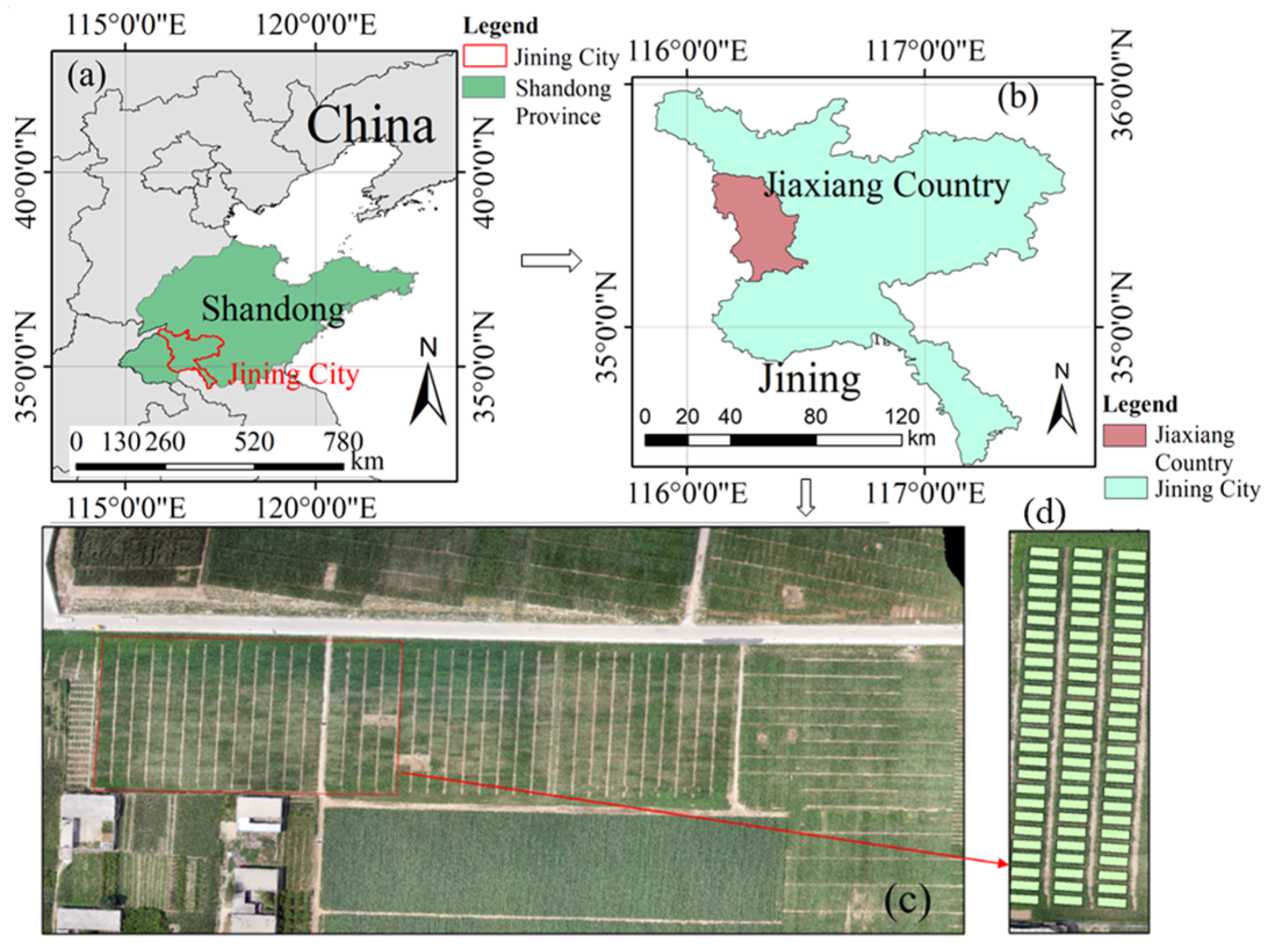
The study site is located in Jiaxiang County (116°22′10″–20″E, 35°25′50″–35°26′10″N), Jining City, Shandong Province, China (
Figure 1). The field site lies on the Yellow River alluvial plain and the soil is a clay loam (pH 7.9), which has a temperate subhumid continental monsoon climate with four distinct seasons: warm spring, hot summer, cool fall and cold winter. It has an average altitude of 35 m, an average annual precipitation of 701 mm and an average annual temperature of 13.9 °C. The annual mean sunshine duration at the site is 2405.20 h, and the annual frost-free period is 210.70 d. We provide the weather information (data from
https://cds.climate.copernicus.eu/ accessed on 6 May 2023) during the experiment in
Figure 2.
2.1.2. Experimental Design
A set of 275 soybean genetic materials with extensive genetic diversity were used as the study materials. According to the length of the growth and development period of soybean varieties, these materials were divided into three groups, including an early maturity group, median maturity group and late maturity group. The approximate growth periods of the early, median and late maturity groups were 90–105 days, 105–120 days and more than 120 days, respectively. Each plot contained material from one genotype, and the size of each plot was 5 m × 2.5 m. The row spacing was 0.5 m and each plot had 5 rows. The plant density was 190,000 plants ha−1. The sowing date of soybean was 13 June 2015. The field experiments used a complete randomized block design with three replicates. We performed field management procedures, including weed control, pest management, irrigation modes and the application of nitrogen, phosphate and potassium fertilizer following local standard practices for soybean production. In total, 33 representative materials (14 early maturity genotypes, 14 median maturity genotypes and 5 late maturity genotypes) from different maturity groups were selected for the study. The selected varieties have differences in podding characteristics (finite, sub-finite and infinite), plant height, flower color, leaf shape, 100-seed weight, effective pod number per plant, seed number per plant, disease resistance, lodging resistance, maturity, etc. For example, in the early maturity group, there were some hybrids with Zhonghuang 13 or Kefeng 14 as parents; in median maturity group, there were some hybrids with Yudou 22 or Jinyi 30 as parents; and in late maturity group, there were some hybrids with Kexin 4 or Fendou 55 as parents.
2.2. Data Acquisition
This section consists of two parts, which introduce the acquisition processes for the UAV data and yield data in the experiment, respectively.
2.2.1. UAV Data Collection
In the study, the field crop-canopy RGB images and hyperspectral images were collected using a snapshot hyperspectral sensor (Cubert UHD 185) and a high-definition digital camera (SONY DSC-QX100, Tokyo, Japan) mounted on an eight-armed DJI S-1000 UAV (Dajiang Innovation, Sham Chun, China). The operating range of the UHD 185 is from the visible to the NIR wavelengths (450–950 nm). The detailed information of the sensors is provided in
Table 1. In addition, a Trimble GeoXT6000 GPS receiver was used to determine the location of the ground control point (GCP) of the test field.
Flight missions were carried out from 11:00 to 14:00 under clear, cloud-free conditions. All flights were flown at a 50 m height to obtain high-quality photos. Before obtaining the hyperspectral data using the UAV, the dark-current collection and standard whiteboard calibration were performed to ensure accurate reflectance data at each growth period. The flight was conducted according to the planned route. The remote sensing data using the UAV were collected at three critical growth periods of soybean during 2015 (1 August 2015 (flowering stage), 1 September 2015 (podding stage) and 17 September 2015 (bean-filling stage)).
2.2.2. Yield Data Collection
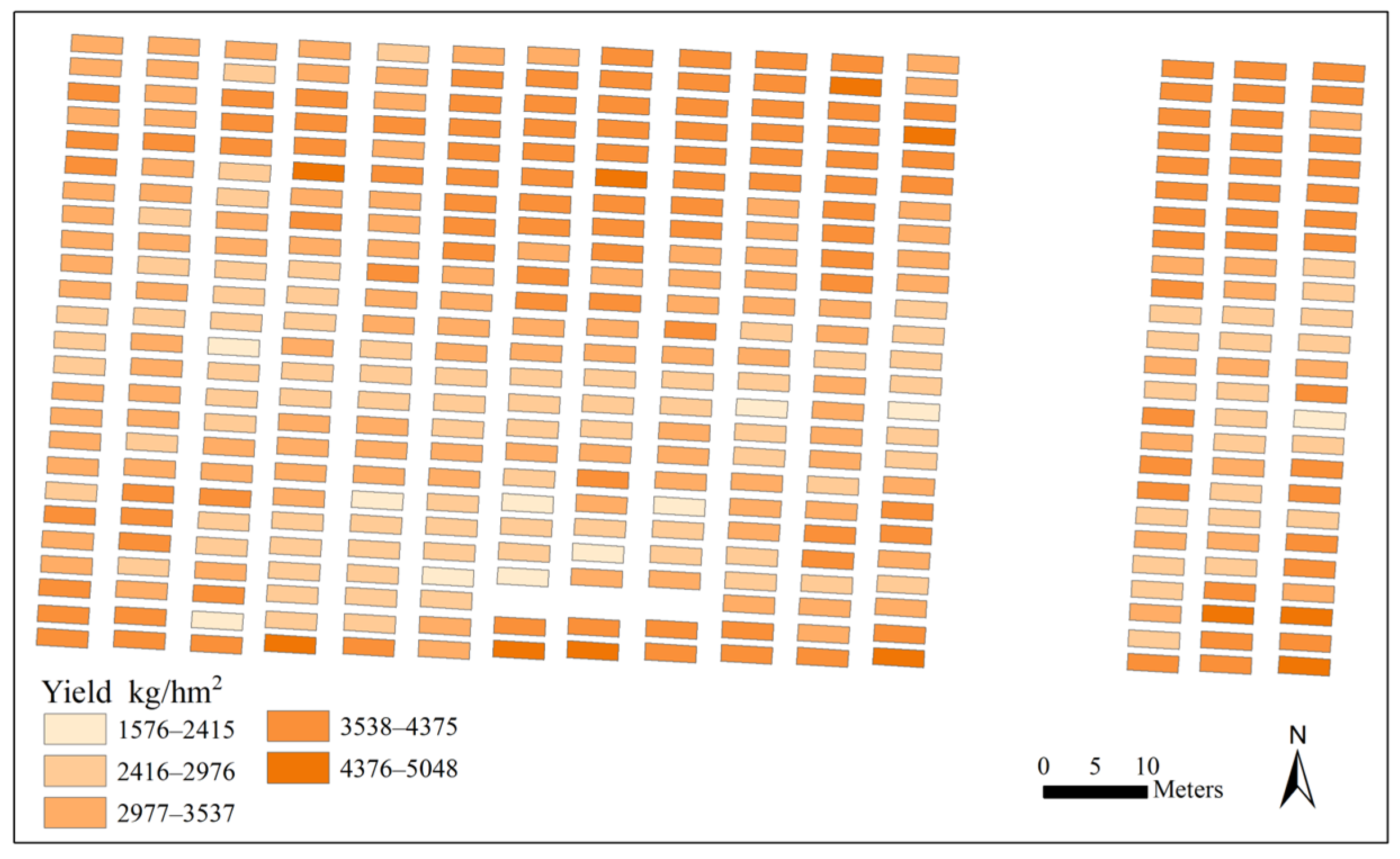
Grain yield for each plot was measured by harvesting three middle rows, with a calculated area of 7.5 m2, when the soybean genotypes in the experimental plot were matured. The soybean plants were harvested and the plot seed yield was measured with the seed moisture adjusted to 13% and was expressed as kg/hm2 for further analysis.
2.3. Image Processing and Feature Extraction
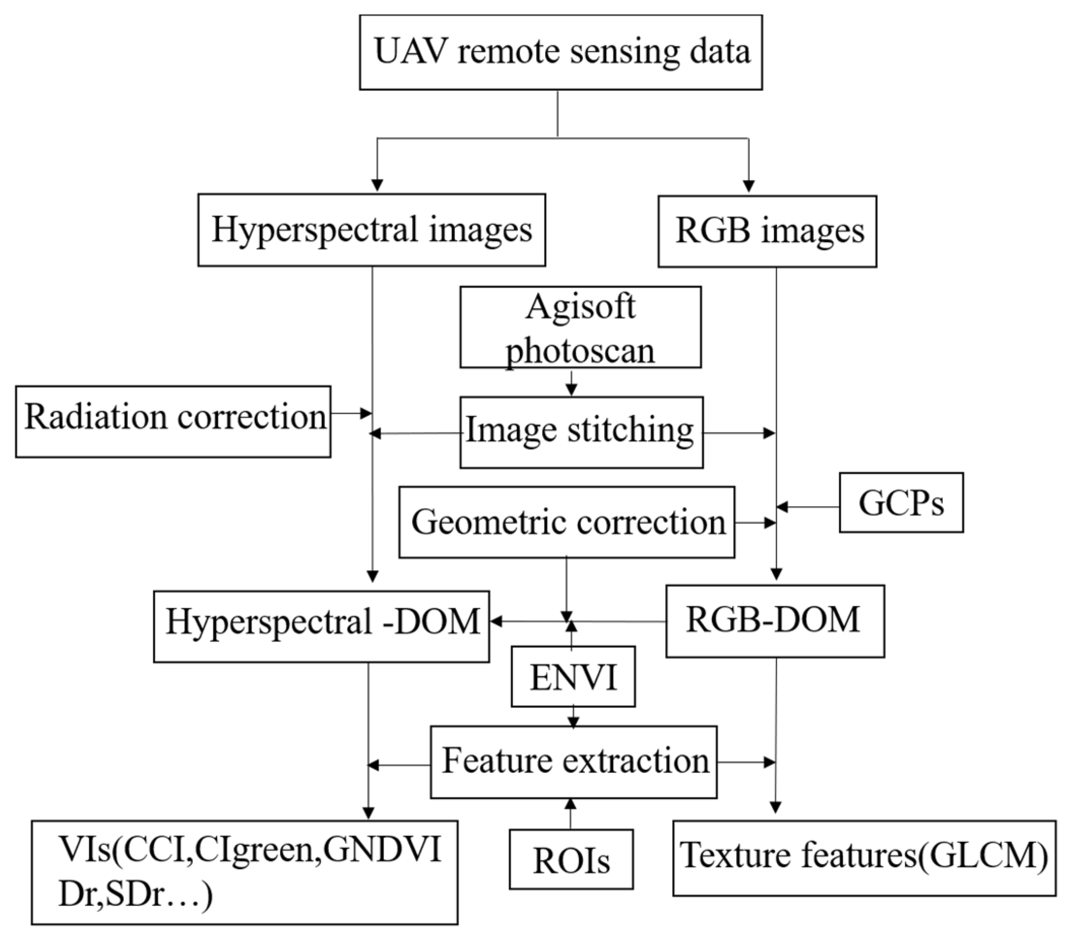
After the flight, the UAV hyperspectral data were processed by geometric correction, image stitching and spectral data extraction. First, the surface reflectance of the hyperspectral images was calibrated based on black-and-white panel data. Then, we calibrated the collected images and processed them into several ortho-mosaic maps. The canopy hyperspectral and digital images of soybean were stitched together using Agisoft PhotoScan software (version 1.5.5, Agisoft LLC, St. Petersburg, Russia) to generate the hyperspectral and RGB digital orthophoto images (DOMs) of the experimental site, respectively. The UAV-based RGB DOMs were rectified by applying a field-measured GCPs in the ENVI software (version 5.3, Harris Geospatial Solutions, Boulder, CO, USA). And, the UAV-based hyperspectral DOMs were rectified by using the UAV-based RGB DOMs. Finally, the regions of interest (ROIs) in all soybean plots were manually delineated in ENVI and the corresponding reflectance data were extracted from the hyperspectral DOMs using the ROI tools. We calculated the average of all pixel values in plots as the extraction results.
In this study, we used three types of features, including VI based on the hyperspectral images as the first type, texture features (Te) based on the RGB images for the second type, and the known maturity group information (M) for the third type. In order to fully explore these parameters, a set of VI including red-edge position (REP), red-edge amplitude (Dr), the minimum red-edge amplitude (Drmin), red-edge area (SDr) and the ratio of the red-edge amplitude and the minimum red-edge amplitude (Dr/Drmin) were selected (
Table 2). REP is the wavelength of the maximum first derivative of the spectrum in the range of 680–760 nm [
34]. Drmin is the value of the minimum red-edge amplitude [
35]. Texture features reflect the spatial dimensional information of the images, which can describe the spatial distribution. In this study, the commonly used gray-level co-occurrence matrix (GLCM) was used to extract Te from RGB images of the red, green and blue bands in ENVI 5.3, which include the mean, variance, homogeneity, contrast, dissimilarity, entropy, second moment and correlation. The same ROIs used for reflectance extraction were applied to extract the texture features of each plot. As for the third type, to maintain data uniformity, we simplified the maturity group information into numbers of 1, 2 and 3 to represent the early maturity group, median maturity group and late maturity group, respectively. The details of the features are listed in
Table 2. The main process of image processing and feature extraction in this study is given in
Figure 3.
2.4. Data Analysis and Model Establishment
This section covered three parts, including statistical analysis of the data, feature selection, and the model building process.
2.4.1. Statistical Analysis
To explore the differences in GY of soybean genotypes between the three maturity groups, a one-way analysis of variance (ANOVA) with an honest significant difference Tukey test was carried out to evaluate it. The threshold for statistical significance was p < 0.05.
For a further understanding of the significance of variation between genotypes, replicates and their interactions for remote sensing features and grain yield, broad-sense heritability (
H2) was computed. The heritability was estimated through the following formula:
where
is the number of replicates, and
and
are the genotypic and error variance components, respectively [
59]. The above data analysis processes were conducted in R software (4.0.4).
2.4.2. Feature Selection
Feature selection is an important part in machine learning. In this study, we adopted the least absolute shrinkage and selection operator (LASSO) algorithm to select sensitive features for yield estimation. The LASSO algorithm executes both variable selection and regularization to improve model accuracy and interpretability [
60]. Under the constraint condition that the sum of absolute values of regression coefficients is less than a constant, some regression coefficients which are equal to zero are generated by adding a penalty term (the
norm ||β||
1) to the least square linear regression (Equation (2)), minimizing the sum of residual squares.
where
is the response of the
th variable,
is the intercept of the model,
is the coefficient of the
th predictor,
= 1, 2, …,
and
is the value of the
th predictor of the
th variable.
λ is a tuning parameter. When
λ = 0, the penalty term has no impact, and the model will produce the least squares estimates. However, as
λ changes to
, the effect of the shrinkage penalty increases, and the coefficients of features hardly contributing to the model will become equal to zero. The feature selection process was conducted in python 3.8 using the “LassoCV” function with a specified range of model parameters of
λ,
and
= 100,000 to optimized the models’ hyperparameters, as well as other default parameters. Finally, the parameter
λ with the least error is selected and the selected feature and coefficients are returned.
2.4.3. Model Construction for GY Estimation
The LASSO method was used to select important variables which were used as inputs to the yield estimation models. As mentioned above, we divided all the features into three types, and the feature selection was executed between the first and the second type of features. The maturity group information, as the third type of feature, was introduced in the machine learning models together with the selected variables to build the soybean yield estimation models.
In the study, the partial least square regression (PLSR), Gaussian processes regression (GPR), random forest regression (RFR) and kernel ridge regression (KRR) were adopted to construct the prediction models at three growth stages and multiple growth stages. The PLSR method combines the advantages of multiple linear regression, canonical correlation analysis and principal component regression. It projects the predictor variables and observed variables into a new space. It can reduce multicollinearity between variables and determine the optimal number of components by minimizing the sum of squares of predicted residuals. GPR is a probabilistic kernel machine based on Bayesian and statistical learning theory. It is a non-parametric model for regression using Gaussian priori process. In the process of estimation, GP maximizes the type-II maximum likelihood through the boundary likelihood of observations. Moreover, it can calculate the posterior distribution of unknown variables and adjusts the hyperparameters. RF is an ensemble method, where many decision trees are integrated into a forest and combined to predict the final outcome. The final prediction results are the averaged value of all the trees. SVR is a regression algorithm derived from SVM, which uses kernel function to map data to a high-dimensional space and realizes regression by finding the optimal hyperplane. The introduction of an insensitive loss function and regularization enables it to solve nonlinear regression problems. KRR has an identical model form to SVR, but it uses square error loss as a loss function. It shrinks the coefficients by applying penalties to constrain their possible values. All the yield estimation models were built in Python 3.8.
2.5. Model Evaluation
We used two commonly used metrics, R
2 and RMSE, to compare the performance of the GY estimation models. We optimized the models’ hyperparameters and evaluated all the models by a 10-fold cross-validation method and used the mean results of the cross-validation in the model comparisons. The calculation formula of R
2 and RMSE are as follows:
where
is the number of samples;
and
are the measured and the predicted grain yield of sample
, respectively; and
represents the mean of the measured grain yield. The model with a higher value of R
2 and lower values of RMSE can predict grain yield better.


 ,
, 


