Remote Sensing Parameter Extraction of Artificial Young Forests under the Interference of Undergrowth

Abstract

Due to the lower canopy height at the maximum crown width at the bottom of young Picea crassifolia trees, they are mixed with undergrowth. This makes it challenging to accurately determine crown size using CHM data or point cloud data. UAV imagery, on the other hand, incorporates rich color information and, after processing, can effectively distinguish between spruce trees and ground vegetation. In this study, the experimental site was an artificial young forest of Picea crassifolia in Shangshan Village, Qinghai Province, China. UAV images were used to obtain normalized saturation data for the sample plots. A marker-controlled watershed segmentation algorithm was employed to extract tree parameters, and the results were compared with those obtained via point cloud clustering segmentation and the marker-controlled watershed segmentation algorithm based on Canopy Height Model (CHM) images. The research results showed that the single tree recognition capabilities of the three types of data were similar, with F-measures of 0.96, 0.95, and 0.987 for the CHM image, UAV imagery, and point cloud data, respectively. The mean square errors of crown width information extracted from the UAV imagery using the marker-controlled watershed segmentation algorithm were 0.043, 0.125, and 0.046 for the three sample plots, which were better than the values of 0.103, 0.182, and 0.074 obtained from CHM data, as well as the values of 0.36, 0.461, and 0.4 obtained from the point cloud data. The point cloud data exhibited better fitting results for tree height extraction compared to the CHM images. This result indicates that UAV-acquired optical imagery has applicability in extracting individual tree feature parameters and can compensate for the deficiencies of CHM and point cloud data.

1. Introduction

Forest ecosystems have a prominent position in the global carbon cycle, and artificial young forests, as a type of forest ecosystem, are important terrestrial carbon sinks in carbon-neutral systems [1,2,3,4]. By measuring individual tree feature parameters, forest biomass and carbon content can be estimated [5]. These parameters also serve as the foundation for forestry carbon sinks and can be used to determine carbon offset quotas in forest carbon trading. Typically, measurement methods for forest carbon sink projects include biomass estimation [6], forest stock estimation [7], and carbon emission estimation algorithms [8]. Among these methods, biomass estimation algorithms provide the most accurate forest carbon estimates due to their use of precise data [9,10]. Additionally, remote sensing techniques, with their timeliness and large-scale synchronous observations, can periodically obtain individual tree feature parameters, replacing inefficient manual surveys, reflecting the cumulative carbon storage in artificial forests over long periods. Thus, these methods are well-suited for forestry carbon accounting and trading [11,12,13].

Mao Chunyan [2] and Zheng Xueting [4] determined the allometric growth equation of juvenile Qinghai spruce by drying and weighing various parts of the juvenile trees. Based on their derived equation, it is possible to estimate the biomass of a single tree by inputting parameters such as crown width, tree height, and ground diameter. Notably, Zheng Xueting and colleagues proposed an allometric growth equation that only requires crown width and tree height. This equation effectively addresses the challenge of remote sensing techniques in obtaining tree ground diameters.

Currently, there are two commonly used approaches for individual tree segmentation based on LiDAR point cloud data containing forest tree information [14,15]. The first approach involves generating a CHM from the LiDAR point cloud data. This approach is based on the fact that tree tops are represented as local maxima, forming local high values in the point cloud data. By using a fixed or variable window, local maxima can be searched in the image to determine the positions of individual trees. Then, tree outlines can be delineated based on tree image features to obtain tree feature information [16,17,18]. The second approach directly performs clustering analysis on the point cloud data, segmenting individual trees based on their spatial distribution characteristics to extract tree feature information. Both of these approaches are widely used in tree feature extraction [19]. Previous research has analyzed the applicability of different segmentation algorithms for these two types of data. Li Pinghao et al. found that in most sample plots, the results of point cloud clustering segmentation and the watershed segmentation algorithm were superior to those of the fourth-degree polynomial fitting segmentation method [5]. Yan et al. proposed an automatic hierarchical individual tree segmentation method based on point cloud data that clusters the point cloud using the mean shift algorithm and iteratively segments the point cloud using the NCUT algorithm, achieving an average correctness of 0.90 [17]. Geng Lin et al. used a marker-controlled watershed segmentation algorithm to extract the three-dimensional structure of tree crowns and then extracted the effective crown of the forest stand based on the results [20]. In existing research, it can be observed that the distance clustering segmentation algorithm based on point cloud data and the marker-controlled watershed algorithm have robust applicability in forest stands with different characteristics [21,22,23,24]. Ana et al. presented a method for automatically detecting the positions and broad crown information of individual Eucalyptus trees from point clouds acquired by a portable LiDAR system. This approach can be widely applied in mature Eucalyptus stands, enabling accurate estimation of individual tree metrics [25]. Additionally, machine learning has also been applied to individual tree extraction [26]. Given the significance of urban trees for city management, Schmohl et al. [27] introduced a 3D neural network leveraging airborne laser scanning point clouds to achieve accurate individual tree detection, outperforming traditional methods and achieving an average precision of 83% in an urban setting. Windrim et al. focused on isolating single trees, identifying stem points, and constructing a segmented model of the primary tree trunk that encompasses both tree height and diameter. Their methodology involved a sequence of deep learning stages, beginning with ground characterization and removal, followed by individual tree delineation, and concluding with the segmentation of tree points into stem and foliage components [28]. A comprehensive approach combining airborne LiDAR and hyperspectral data was proposed by Man et al. for accurate urban vegetation extraction at both two-dimensional and three-dimensional levels, demonstrating high accuracy in classification and individual tree delineation, offering valuable insights for urban vegetation management and spatial planning [29]. However, most previous studies focused on tall and wide-crowned mature forests, and the proposed methods were mostly specific to certain tree species, lacking research applicability in artificial young forests with low average heights and small crown widths. Artificial young forests have low carbon storage per unit area but a large distribution area and great potential for carbon storage. Such forests are important terrestrial carbon sinks in carbon-neutral systems, and accurately calculating the carbon storage of artificial young forests is of great significance for achieving carbon neutrality goals.

Picea crassifolia crowns have a conical shape, and in young Picea crassifolia forests, the height of branches beneath the crown is lower than that of the surrounding ground vegetation. In the point cloud data, the maximum crown widths of the branches and leaves are mixed with the undergrowth, making them difficult to distinguish. Extracting tree crown width information using point cloud data and CHM data generated from point clouds will, therefore, result in significant errors. Consequently, traditional segmentation methods can struggle to meet the requirements for extracting crown width parameters in young Picea crassifolia forests in practical applications.

Based on this, the present study attempts to use new data for extracting canopy width parameters of young Picea crassifolia trees, aiming to address the issue of branch and ground vegetation mixing at the maximum canopy width of young Picea crassifolia. To achieve this, the UAV imagery undergoes a normalization saturation processing, followed by single tree segmentation using the marker-controlled watershed segmentation algorithm to extract canopy width parameters. To validate the accuracy of this method, both the commonly used marker-controlled watershed segmentation algorithm for segmenting CHM data and the point cloud distance clustering-based segmentation algorithm for extracting single tree feature parameters from point clouds are employed. This comparison aims to assess the performance of using UAV imagery for canopy width extraction under the influence of undergrowth. The remaining sections of this paper are structured as follows. Section 2 introduces the study area and the processing workflow of UAV imagery and point cloud data. In Section 3, a comparison is made between the differences in extracted individual tree crown width and elevation parameters from different data sources and the measured data. Section 4 discusses the impact of plot and tree species characteristics on the extraction of individual tree feature parameters. Finally, Section 5 provides a summary of the conclusions drawn in this paper and work that could be conducted in the future.

2. Materials and Methods

The present study takes artificial young Picea crassifolia forests around Xining City in Qinghai Province as the sample. Leveraging the characteristics of UAV imagery, which provides rich color and texture information and is easy to obtain, this study analyzes the applicability of UAV imagery in extracting tree parameters in young forests and addresses the challenges arising from a mixture of tree crowns and undergrowth. To achieve these goals, this research utilizes UAV optical imagery and applies a marker-controlled watershed algorithm to segment and extract tree feature parameters from visible light images. The results are compared with traditional CHM watershed segmentation and point cloud segmentation results to verify the feasibility of this method in extracting crown width information in artificial young forests. However, since UAV imagery does not include vegetation height information, tree height information is extracted and analyzed from CHM data and LiDAR data.

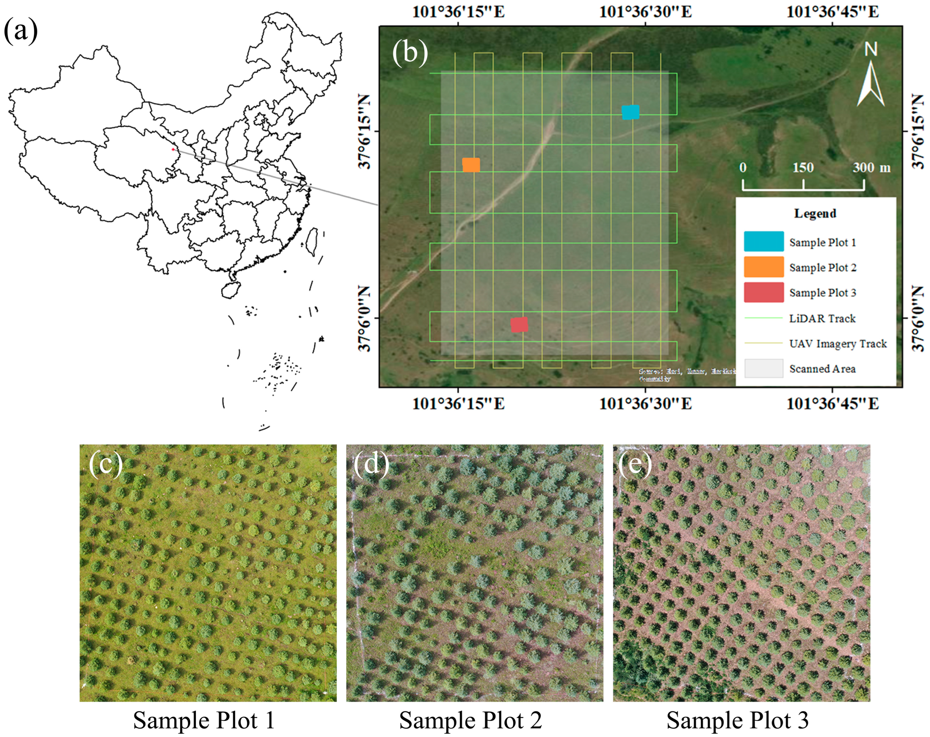
2.1. Study Area Overview and Data Collection

This study selected artificial young Picea crassifolia forests in the vicinity of Shangshan Village, Qinghai Province, China (101°36′~101°37′E, 37°05′~37°06′N), as the experimental area. The vegetation in the study area is mainly composed of artificially planted Picea crassifolia. Most of these trees were planted in 2004, but due to natural disasters such as hail and frost, some young trees died. Replanting was conducted in 2014, and currently, the average stand density is approximately 2000 trees per hectare. Three sample plots measuring 30 × 30 m were selected within the study area based on planting time, average stand density, and the complexity of vegetation within the plots. Sample Plot 1 has more replanted trees, and its average tree height is the lowest among the three plots. In Sample Plot 2, both average height and crown width are relatively higher. Some individual tree crowns at the northeast and southwest corners of the plot are entangled, which may pose challenges for extracting tree feature parameters. In Sample Plot 3, there are fewer replanted trees, resulting in better uniformity. However, in the southwest corner of the plot, there is an area of approximately 5 × 5 m covered with shrubs, and these shrubs are mixed with the artificially planted Picea crassifolia. Figure 1 shows the location schematic and overhead view of the sample plots.

The data used in this study include field measurements collected from the study area’s sample plots, LiDAR data used for extracting single tree feature parameters, and UAV imagery data. To validate the accuracy of the extracted individual tree feature parameters based on different data sources, this study referred to the primary content, methods, and technical specifications of plant community inventory proposed by Fang Jingyun [30] and established field-measured sample plots. The field measurements were conducted in July 2022. Each sample plot within the experimental area was set as a square with an area of 900 m². The dominant tree species in the plots was Picea crassifolia, with a few plots containing wild sea buckthorn and other shrubs. In each plot, the following measurements were taken: slope and aspect data, measured using a compass. The slope of the sample plots is used to plan the size of the plots. The length of each side of the sample plots is calculated based on the cosine values corresponding to different slopes, ensuring that the projected shape of the plots in the imagery remains a 30 × 30 m square. Additionally, the aspect of the sample plots is used to assist in calibrating the compass level, ensuring the accuracy of the positioning of the plot vertices. Tree height was measured using a clinometer, crown width in the east–west and north–south directions was measured using a steel tape measure, and tree Diameter at Breast Height (DBH) was measured using a caliper. During the measurements, the sequence of tree measurements within each plot was recorded, and an aerial view map was drawn to aid in later data matching. Handheld Real-Time Kinematic (RTK) [31] measurements were used to record the latitude and longitude information of the four corners of each plot for geometric correction of the image [32]. Compared to mature spruce, young Picea crassifolia displays significant differences in various parameters. To more intuitively reflect this distinction and the planting characteristics of young Picea crassifolia in artificial forests, statistical data for each feature parameter were calculated. A statistical summary of the field-measured single tree structural data is shown in

Table 1. Measured data statistics.

Plots	Parameters	Minimum	Maximum	Mean	Median	Standard Deviation	Number
1	DBH/cm *	0.84	3.50	1.74	1.64	0.60	216
	DGH/cm **	1.08	7.95	5.24	5.33	1.14
	Tree height/m	0.41	2.85	1.47	1.51	0.48
	Crown width/m	0.19	1.92	1.22	1.24	0.30
2	DBH/cm *	1.13	8.27	3.19	3.19	1.08	175
	DGH/cm **	1.48	9.96	6.55	7.08	1.86
	Tree height/m	0.48	3.93	2.44	2.62	0.70
	Crown width/m	0.36	2.54	1.63	1.71	0.46
3	DBH/cm *	1.26	5.07	2.84	2.75	0.69	232
	DGH/cm **	3.03	10.07	6.64	6.66	1.14
	Tree height/m	1.47	3.35	2.42	2.44	0.33
	Crown width/m	1.21	2.60	1.66	1.66	0.19

* The diameter of the trunk of a tree at 1.3 m. ** The diameter of the trunk of a tree at the ground.

. The parameters in the table correspond to tree components, as illustrated in Figure 2.

The LiDAR data were acquired on 8 August 2022 using a DJI M300 RTK unmanned aerial vehicle equipped with a DJI L1 LiDAR sensor. Detailed parameters of the L1 LiDAR sensor are shown in

Table 2. Main specifications of L1 LiDAR sensor.

LiDAR
Point Cloud Data Rate	Single Return: Up to 240,000 points/s Multiple Returns: Up to 480,000 points/s
System Accuracy	Planar Accuracy: 10 cm @ 50 m Vertical Accuracy: 5 cm @ 50 m
Range Accuracy	3cm@100m
Maximum Returns	3
FOV *	Non-repetitive Scan: 70.4° (horizontal) × 77.2° (vertical) Repetitive Scan: 70.4° (horizontal) × 4.5° (vertical)
Laser Power	Repetitive Scan: 9 W Non-repetitive Scan: 8 W

* Field of view. The UAV imagery data comprising optical images containing three RGB channels were acquired from 22–29 July 2022 using a DJI Phantom 4 UAV. The flights were conducted at a relative altitude of 60 m. The imagery sensor had an effective pixel count of 20.48 million, with an image resolution of 5472 × 3648 pixels, corresponding to a ground resolution of 3 cm.

. The young Picea crassifolia trees are generally small in size, and to obtain high-precision extraction results, it was necessary to acquire high-density point cloud data. Additionally, to minimize errors, the data for the three sample plots were collected in a single aerial survey mission. The data collection took place under favorable weather conditions, with a relative flight altitude of 70 m and a flight speed of approximately 4 m/s. The LiDAR sensor recorded three echoes per pulse, resulting in an average point density of 1300 points per square meter. Subsequently, the acquired data were clipped to extract the point cloud data within the study area.

2.2. Methods

This study utilized LiDAR data and UAV imagery. From the LiDAR data, a Canopy Height Model (CHM) was extracted. The Marker-controlled Watershed Segmentation algorithm was then employed to extract tree feature parameters from both the CHM data and the UAV imagery [5,33]. The point cloud after noise point removal, ground point separation, and normalization was segmented using the point cloud clustering segmentation algorithm, and parameters were extracted [34]. The specific workflow is illustrated in Figure 3. In addition, this study utilized the LiDAR 360 V5.2 software platform for point cloud data preprocessing, generating CHM data, and segmenting point cloud and raster data. The UAV imagery was processed using Pix4D and ENVI 5.2. The visualization of point cloud segmentation results was implemented using the lidR package in R programming language, and the validation of individual tree feature parameters extraction results was also performed in R.

2.2.1. Removing Noise Points, Normalization, and CHM Generation of Point Cloud Data

When the LiDAR sensor emits laser pulses and receives echo signals from the target objects on the ground, the reflections from low-flying objects, such as birds or insects, can be mistakenly recorded as reflections from the target objects being measured. Additionally, data points can deviate from the target objects due to flight errors and sensor inaccuracies. These data points can have an impact on the research results and accuracy. Therefore, it is necessary to select appropriate parameters and remove noise points to improve the data quality before conducting experiments. In this study, a spatial distribution-based algorithm was used to remove noise points from the data. This algorithm calculates the average distance from each point to its K nearest neighbors by using K nearest neighbor statistics for each point. Points with an average distance outside the threshold range are removed. Through multiple experiments, it was determined that the optimal noise removal in this study was achieved by setting the K nearest neighbor count to 50 and the standard deviation multiple to 15.

In this study, the Cloth Simulation Filter (CSF) algorithm [35] was used to filter the LiDAR data. This algorithm, proposed by Zhang et al., uses a spring-mass model to simulate a cloth covering the flipped point cloud surface. By adjusting the forces between the mass points, this algorithm adapts to the varying roughness of the ground surface, separating the point cloud into ground points and non-ground points. The ground points are interpolated using Kriging to generate the DTM data, while the non-ground points, representing objects, retain the first return echoes and are interpolated using Kriging to obtain the DSM data. The CHM is a surface model that represents the distance from the vegetation canopy top to the ground surface, capturing the variations in the vegetation canopy. The calculation formula for CHM is as follows [36]:

$$\mathrm{C}\mathrm{H}\mathrm{M}=\mathrm{D}\mathrm{S}\mathrm{M}-\mathrm{D}\mathrm{T}\mathrm{M}$$

(1)

where CHM represents the Canopy Height Model, DTM stands for the Digital Terrain Model, and DSM represents the Digital Surface Model. DTM is a vector dataset composed of irregularly spaced 3D mass points. In contrast, DSM includes the heights of objects such as buildings and trees on the ground surface. To mitigate the influence of pseudo-canopy vertices and ground noise points in the Canopy Height Model, Gaussian filtering was applied to remove noise and enhance data quality.

Additionally, preprocessed point cloud data contain height information for the underlying surface beneath the trees, preventing accurate tree height information from being obtained during segmentation. Normalization can remove the influence of terrain variations on the elevation of point cloud data. The principle of this method is to subtract the elevation of the nearest ground point from the elevation value of each point. This operation involves subtracting the point cloud data from the Digital Terrain Model (DTM), resulting in the extraction of tree height information.

2.2.2. UAV Imagery Processing

After geometric correction and preprocessing to eliminate distortions, the UAV imageries were converted from the RGB color space to the HSV color space [37,38]. In this process, the R, G, and B attributes first need to be normalized. Then, the values of H (hue), S (saturation), and V (value) are calculated separately as follows:

$$V=max(R\prime ,G\prime ,B\prime )$$

(2)

$$S=\left\{\begin{array}{cc}\frac{V-min(R\prime ,G\prime ,B\prime )}{V}& ,\mathrm{if}V\ne 0\\ 0& , \mathrm{else} \end{array}\right.$$

(3)

$$H=\left\{\begin{array}{cc}60\times (G\prime -B\prime )/(V-min(R\prime ,G\prime ,B\prime \left)\right)& , \mathrm{if}V=R\prime \\ 120+60\times (B\prime -R\prime )/(V-min(R\prime ,G\prime ,B\prime \left)\right)& , \mathrm{if}V=G\prime \\ 240+60\times (R\prime -G\prime )/(V-min(R\prime ,G\prime ,B\prime \left)\right)& , \mathrm{if}V=B\prime \end{array}\right.$$

(4)

where R′, G′, and B′ represent the transformed red, green, and blue channels, while H, S, and V represent hue, saturation, and value, respectively. Afterward, the obtained HSV image is processed to obtain the normalized saturation, calculated according to the following formula:

$$S\prime =S/H$$

(5)

where S′ represents the normalized saturation, S represents saturation, and H represents hue. In the color space, saturation refers to the purity or intensity of a color, representing the degree of color intensity relative to gray. Normalized saturation is achieved by mapping the original color data to the range [0, 1], which standardizes the saturation of different colors, facilitating comparison and analysis to better understand and describe the intensity of colors. With the use of normalized saturation, higher values indicate higher purity and intensity, while lower values indicate lower purity and intensity, allowing for a more reliable comparison of color purity and intensity between different colors. This process helps reduce the influence of hue and facilitates a comparison of color purity and intensity. In this study, due to the significant color differences between spruce trees and undergrowth in the image, calculating the normalized saturation was able to effectively extract the outline of spruce tree crowns for individual tree parameter extraction. Finally, the image was subjected to mean filtering to eliminate the impact of image noise.

2.2.3. Marker-Controlled Watershed Segmentation Algorithm

To explore the accuracy of different data in single tree recognition and the extraction of tree parameters, this study employed the marker-controlled watershed segmentation algorithm to process the CHM data and UAV imagery and extract single tree features [39]. The watershed segmentation algorithm is a terrain-based image segmentation algorithm. The basic concept of this algorithm is to treat the grayscale values of an image as height values. The connected lines of pixels with higher grayscale values can be considered as ridges or watershed lines. The local minima and the surrounding regions influenced by these lines are referred to as catchment basins. The algorithm starts by injecting water from the local minima and gradually raises the water level. When the water level reaches a neighboring pixel, the algorithm determines whether to submerge the pixel based on whether the distance between the pixel and the local minimum is less than a set threshold. To prevent water from overflowing and merging with neighboring catchment basins, “dams” can be constructed on the watershed lines. This process continues until the water level reaches the maximum grayscale value. The resulting dams and original watershed lines divide the entire image into different regions, achieving image segmentation. An illustration of the watershed algorithm is shown in Figure 4 [40].

During the segmentation process using the watershed algorithm, excessive local minima can appear in the image due to noise or interference from other objects on the ground. This leads to the formation of independent regions, resulting in over-segmentation of the image. To address this issue, in this study, the image was subjected to Gaussian smoothing to remove redundant local minima and merge the regions generated by these minima. By adjusting the Gaussian smoothing factor and the window radius, the optimal segmentation result was obtained, minimizing the impact of over-segmentation in the image.

2.2.4. Point Cloud Clustering Segmentation Algorithm

The tree structure of Picea crassifolia resembles a cone lying flat on the ground, as illustrated in Figure 5. Li et al. proposed a distance-based discriminant clustering algorithm using point cloud data, which is well-suited for this type of data. The algorithm works as follows (Figure 6). Firstly, the global maximum value A is identified in the data, which serves as the vertex of the first tree. According to the critical spacing value and the principle of minimum spacing, data points below A are classified one by one. For example, in Figure 6, point B is assigned as the vertex of the second tree because the distance between AB exceeds the pre-set critical spacing value. Next, we compare the height of point C, which is lower than B. Additionally, the distance between C and A is smaller than the distance between C and B, and the distance between C and A is within the critical spacing value. Therefore, C is classified into the tree cluster of A. Further, point D is closer to B than to C, so D is classified into the tree cluster of B. In this way, the point cloud data are segmented. The critical spacing value used for segmentation should be similar to the crown radius of the trees in the sample plot to avoid under-segmentation or over-segmentation situations [34].

2.2.5. Segmentation Result Accuracy Verification

To verify the accuracy of the identification results for different datasets, this study compares the identification results with field measurements. Here, the accuracy of the identification results is evaluated using Precision (p), Recall (r), and F-measure (F) [41]. Precision refers to the proportion of correctly identified individual trees to the total number of identified trees. Recall represents the proportion of correctly identified individual trees to the total number of trees in the sample area. The F-measure is a metric used to evaluate the classification results and can reflect the effectiveness of the segmentation method. The formulas for calculating the evaluation metrics are as follows:

$$p=\frac{D_T}{D_T+D_F}$$

(6)

$$r=\frac{D_T}{D_T+D_M}$$

(7)

$$F=2\frac{r\times p}{r+p}$$

(8)

where p represents precision, r represents recall, and F represents the F-measure. D_T denotes the number of individual trees correctly identified by the segmentation algorithm, D_F represents the number of individual trees erroneously segmented, and D_M represents the number of individual trees not identified in the sample area.

For the accuracy evaluation of extracting tree feature parameters, this study uses least squares linear regression to fit the relationship between the crown width, tree height parameters extracted using different algorithms and data, and measured data. The Mean Squared Error (MSE) is then calculated to assess the quality of the extraction results:

$$MSE=\frac{1}{n}\sum _{i=1}^n{\left(Y_i-{Ŷ}_i\right)}^2$$

(9)

where MSE represents the mean squared error, Y_i represents the true value, Ŷ_i represents the predicted value, and n represents the total number of individual trees involved in the accuracy evaluation within the sample area.

3. Results

3.1. Analysis of Individual Tree Identification Accuracy Based on Multiple Data Sources in the Sample Plots

Table 3. Accuracy evaluation results of single tree identification.

Plots	Data	Number of Trees	Number of Measurements	p	r	F
1	CHM	216	198	0.991	0.986	0.988
	UAV image	216	199	0.9567	0.943	0.950
	Point Cloud	216	211	0.991	0.977	0.984
2	CHM	175	168	1.000	0.960	0.980
	UAV image	175	184	0.929	0.977	0.953
	Point Cloud	175	168	1.000	0.960	0.980
3	CHM	232	245	0.945	1.000	0.972
	UAV image	232	241	0.930	1.000	0.964
	Point Cloud	232	232	0.994	1.000	0.997

presents the evaluation results of individual tree segmentation accuracy using different methods in the three sample plots. As shown in the table, all three methods provide good overall identification results, with F-values ranging from 0.950 to 0.997 and an overall F-value of 0.969. The individual tree segmentation p ranges from 0.929 to 1, with an overall precision of 0.969. The individual tree segmentation recall varies from 0.903 to 1, with an overall recall of 0.963. The identification results are shown in Figure 7. However, due to issues such as over-segmentation and under-segmentation, some individual tree segmentation results do not match the measured data in certain sample trees.

The identification results of individual trees were influenced by the characteristics of the data and the features of the sample plots. CHM images and point cloud data contain elevation information, allowing the utilization of dynamic window searches for local maxima as tree top points, which enhances the accuracy of tree identification compared to UAV imagery. However, smaller spruces are more likely to be overlooked due to obscuration with low-lying vegetation on the ground, resulting in lower recall rates. The precision may vary slightly among different sample plots due to variations in vegetation complexity. In Sample Plot 1, for example, herbaceous plants near spruce crowns and some surface vegetation had similar colors to the crowns, leading to incorrect identification in the UAV imagery. In the southwest corner of Sample Plot 3, there were significant numbers of wild sea buckthorn plants interspersed with spruces. Both CHM images and UAV imagery mistakenly identified different quantities of sea buckthorn as target objects, resulting in lower segmentation accuracy. Sea buckthorn and other shrubs have distinct differences in height and crown shape compared to spruces, making them easier to distinguish in point cloud segmentation algorithms.

3.2. Evaluation of Single Tree Width Extraction Accuracy Based on Multiple Data Sources

To evaluate the accuracy of the single tree parameters extracted by the algorithms, the measured data were matched with the algorithmically extracted data. Based on an aerial view of the sample plot and through manual matching, the measured data were associated with the corresponding single tree parameters obtained by the algorithm while discarding the results of incorrect identification, over-segmentation, and under-segmentation.

3.2.1. Verification of Crown Width Extraction Accuracy Using Different Data Sources

Figure 8 shows the regression relationship and MSE between the crown width information extracted from CHM, UAV imagery, and point cloud data using the marker-controlled watershed algorithm and point cloud clustering segmentation algorithm. The comparisons were made with field-measured crown widths. In the figure, the MSE of the crown width extracted from UAV imagery is superior to that of the CHM and point cloud data in all three study sites. Here, the MSE values for UAV imagery are 0.043, 0.125, and 0.046, respectively, while the MSE for CHM imagery is slightly higher, and the point cloud segmentation results exhibit the largest discrepancy from the measured data. Additionally, the coefficients of determination (R²) for the crown width extracted from drone imagery were also found to be reliable, with values of 0.703, 0.817, and 0.353 in the three study sites. However, because the relatively small variations in crown width among the trees in Sample Plot 3 resulted in clustered data distribution, the R² values were comparatively lower.

The MSE results indicate that UAV imagery can provide more reliable results in all three sample plots. The extraction of single tree feature parameters from CHM data and point cloud data presents varying degrees of errors influenced by the characteristics of the data. The marker-controlled watershed algorithm was found to underestimate crown widths in CHM images compared to the actual values. This result is mainly due to the mixing of the maximum crown width of spruce with ground vegetation points in the acquired LiDAR data, making it difficult to accurately extract the maximum crown width contours in the CHM image, resulting in crown widths smaller than the actual tree crowns. On the other hand, the point cloud clustering segmentation algorithm was found to overestimate crown widths compared to the actual values. This result is primarily because the points representing spruce crowns and ground vegetation are mixed, making it challenging for the algorithm to precisely locate the boundaries of tree crowns, leading to some ground vegetation being identified as part of the crown and resulting in extracted crown widths larger than the actual values.

3.2.2. Verification of Crown Height Extraction Accuracy Using Different Data Sources

Figure 9 shows the regression relationship between the single tree height extracted by the algorithms from different data sources and field-measured tree heights. The results indicate a good fitting relationship for both algorithms, with R-squared values ranging from 0.7625 to 0.9147. Analyzing the data in the graph, it can be observed that the linear fitting relationship between the tree height extracted by the point cloud clustering segmentation algorithm was generally better than that of the watershed segmentation algorithm. The mean square error for the former was smaller than that of the latter, with values of 0.116, 0.155, and 0.112 for the three sites, compared to 0.251, 1.125, and 0.865 for the watershed segmentation algorithm. Due to the conical shape of the spruce crowns, the bottom features of the crowns were occluded in the data acquired by LiDAR, making it impossible to obtain relevant echo information. After filtering the point cloud data and separating the ground points, different-sized holes were formed. When generating the CHM, the DTM data were obtained by fitting the heights of the surrounding point clouds, resulting in varying degrees of errors between the CHM tree height and actual tree height, leading to poorer fitting performance.

4. Discussion

This study employs UAV imagery to extract crown width parameters of young artificial Picea crassifolia forests, aiming to address the issue of significant errors in conventional data extraction results due to the mixing of surface vegetation with the maximum crown width of spruce trees. The research reveals that factors such as sample plots, tree crown structures, and data types contribute to variations in the extraction results of individual tree feature parameters.

4.1. The Influence of Plot Characteristics on Tree Identification Using Different Data Sources

The three data sources all yielded good results in tree recognition, surpassing previous research. Guo Yushan et al. [33] used the marker-controlled watershed segmentation algorithm to segment willows and black locusts, achieving F-values of 0.878 and 0.655, respectively. Wang Xinyun et al. [42] used a 0.1 m resolution CHM image to segment Chinese pine and larch, with F-values of 0.862 and 0.916, respectively. However, the corresponding accuracy values were lower than those achieved in this study. The main reason for this difference is that the selected sample plots in this study are artificial forests, which have regular planting patterns and larger inter-tree gaps, making them easier to recognize. Additionally, there is less interference from shrubs and other vegetation in artificial forests. However, slight variations in performance among the three algorithms were observed in the different sample plots. The marker-controlled watershed algorithm performed well in identifying spruces and distinguishing shrubs in the sample plots. However, some spruces with smaller crown sizes could be overlooked in the CHM images, resulting in lower recall rates compared to the other two algorithms. When using the marker-controlled watershed algorithm to segment the UAV images, some low-growing shrubs in Sample Plot 1 were mistakenly identified as spruce crowns due to their similar colors to the ground vegetation, affecting the recognition accuracy. Additionally, it is challenging to distinguish the vegetation surrounding some spruces, leading to under-segmentation. In Sample Plot 3, some shrubs were also identified as spruce crowns, impacting the recognition accuracy.

However, the study area selected in this paper is a Picea crassifolia artificial young forest, which is composed of a single species, making the situation relatively simple for individual tree segmentation and feature parameter extraction. It is not possible to determine the applicability of these data in other forests. Nevertheless, Qinghai spruce is extensively planted in the northern Gansu region, Qilian Mountains, and eastern Qinghai, accounting for 44% of the coniferous forest area [43]. Due to its vast carbon storage, accurate estimation of its carbon storage is of significant importance for China’s carbon neutrality efforts.

4.2. The Influence of Tree Characteristics on the Extraction of Individual Tree Feature Parameters from Different Data Sources

As shown in Figure 10, the young Picea crassifolia exhibited a unique shape in LiDAR data, resembling an inverted ice cream cone placed on the ground. This distinctive shape caused this species’ point cloud to mix with the undergrowth point clouds, making it difficult to distinguish the boundaries. When extracting tree crown widths using the three data sources, different features were obtained due to the influence of ground vegetation. When using the marker-controlled watershed algorithm to extract crown widths from the CHM image, the crown contours in the CHM image were obtained based on tree crown heights. However, some crowns that were close to the ground or covered by undergrowth resulted in smaller crown contours in the CHM image compared to their actual sizes. As a result, the extracted crown widths were generally underestimated compared to the measured data. UAV imagery performed well in identifying crown boundaries when there was a significant contrast between ground vegetation and tree crowns. This method accurately extracted single tree information. As shown in Figure 8, the crown width information extracted from UAV imagery offered a lower mean square error than the CHM images and point cloud data in different sample plots. The point cloud clustering segmentation algorithm faced challenges in separating trees from ground vegetation during filtering. Therefore, the algorithm tended to identify ground vegetation as tree crowns, leading to an overall overestimation of the extracted crown widths compared to the measured data. As shown in Figure 11, the point cloud segmentation algorithm based on point cloud data included some spruce point clouds along with the surrounding ground vegetation point clouds and shrub point clouds. These ground vegetation point clouds have varying degrees of impact on the extracted crown width information.

Since UAV imagery does not contain tree height information, the tree height information must be obtained from the CHM data and LiDAR data. The results show that using the marker-controlled watershed segmentation algorithm to extract tree height information from CHM data yields R² values ranging from 0.7625 to 0.8441. The distance-based clustering segmentation method using point cloud data achieved R² values ranging from 0.8249 to 0.9147. For different sample plots, the extraction results from point cloud data were superior to those obtained from the CHM data. The main reason for this result is that the CHM data obtained elevated values from the point cloud data. However, due to the unique crown structure of the spruce trees, it was difficult for the point cloud to penetrate the crown and acquire information about the ground beneath. When obtaining CHM data, the DTM beneath the crown was derived by fitting the elevation of surrounding point clouds, resulting in some errors in the extracted elevation information from the CHM data. Cao et al. [44] used the marker-controlled watershed segmentation algorithm to extract tree height with an R² value of 0.8568. Geng et al. [20] used the same method to extract tree height in a deciduous mixed forest with an R² value of 0.8862. Therefore, both the marker-controlled watershed segmentation algorithm and the distance-based clustering segmentation method based on point cloud data exhibited good performance in extracting tree height information in different sample plots.

4.3. The Differences in the Accuracy of Extracting Individual Tree Information Based on Different Data

This paper mainly focuses on two aspects of individual tree information acquisition from the data. Firstly, individual tree recognition is achieved by segmenting the data using algorithms, and then individual specific tree feature parameters are extracted from the segmented trees. Due to the unique crown shape of spruce trees, extracting individual tree feature parameters, especially crown width, from commonly used CHM data and point cloud data can result in significant errors. As shown in Figure 8, the crown width feature parameters extracted from the CHM image are generally underestimated compared to the actual crown width, and there are many outliers. This may be due to the fact that the DSM data generated from the point cloud cannot identify the crown area covered by undergrowth during CHM generation. Additionally, the missing data on the lower part of the spruce in the DTM image causes the elevation of the lower part of the spruce to be fitted based on the surrounding elevation, leading to errors. Although UAV imagery processed with normalized saturation can effectively identify undergrowth and spruce, its recognition capability for shrubs in Plot 3 is relatively poor. Furthermore, in other plots, some herbaceous plants with colors similar to spruce can also affect the identification of individual trees in UAV data, resulting in a slightly lower F-measure compared to CHM data and point cloud data. However, the crown width extraction results from correctly identified individual trees are more accurate and well-fitted to the measured data in UAV imagery. The crown width extracted from the point cloud data tends to be overestimated due to the influence of ground vegetation, and this causes most of the outliers spreading to the right side of the plot. Additionally, both point cloud data and CHM data can provide good accuracy for individual tree recognition as they reflect the elevation information of the trees.

5. Conclusions

This study took a young Picea crassifolia plantation in Shangshan Village, Qinghai Province, China, as the experimental site. A marker-controlled watershed segmentation algorithm and point cloud clustering segmentation algorithm were used to extract single tree parameters from CHM data, UAV imagery, and point cloud data from the site, and the extraction accuracy was evaluated. The conclusions are as follows.

(1)

All three types of data achieved good results in single tree recognition, with F-values ranging from 0.95 to 0.997, the precision (p) of single tree segmentation ranging from 0.929 to 1, and the recall of single tree segmentation ranging from 0.903 to 1. Since the CHM data and point cloud data contained tree height information, the local maxima obtained through dynamic window searching were used as treetops for single tree recognition. Therefore, the accuracy of single tree recognition was higher for CHM data and point cloud data than for UAV imagery, and the single tree recognition based on point cloud data yielded the best results.

(2)

The crown width extraction results based on UAV imagery were superior to the CHM and point cloud data. The MSE values for the three sample plots were 0.043, 0.125, and 0.046, respectively, which are better than the values obtained for the CHM data (0.103, 0.128, and 0.4) and point cloud data (0.36, 0.461, and 0.4). Additionally, linear regression fitting performed better than the CHM and point cloud data.

(3)

The fitting effect of extracting the single tree height using the point cloud clustering segmentation algorithm was overall better than that of the watershed segmentation on CHM images, with mean squared errors of 0.116, 0.155, and 0.112 for the three sample plots. The overall fitting effect was good, while the CHM data, due to ground holes, were found to result in potentially larger errors during generation, leading to a worse fitting effect.

This study attempts to use UAV imagery to extract individual tree crown widths, aiming to address the issue of significant errors in conventional methods caused by the mixing of surface vegetation and the maximum crown width of young Picea crassifolia trees. UAV imagery was employed to generate normalized saturation data for the study plots, with the objective of enhancing the differentiation between Picea crassifolia trees and surrounding vegetation. This differentiation facilitates the use of the watershed segmentation algorithm for tree crown segmentation. Therefore, acquiring UAV imagery during the autumn season, when most surface vegetation has withered, could potentially lead to improved extraction of Picea crassifolia crown width. Additionally, the impact of UAV imagery resolution on the extraction results is also worthy of exploration.

References

1. Santoro, M.; Cartus, O.; Fransson, J.E. Dynamics of the Swedish forest carbon pool between 2010 and 2015 estimated from satellite L-band SAR observations. Remote Sens. Environ. 2022, 270, 112846. [Google Scholar] [CrossRef]
2. Mao, C.; Yi, L.; Xu, W.; Dai, L.; Bao, A.; Wang, Z.; Zheng, X. Study on Biomass Models of Artificial Young Forest in the Northwestern Alpine Region of China. Forests 2022, 13, 1828. [Google Scholar] [CrossRef]
3. Shu, Q.; Tang, S. The Status and Trend of International Forest Resources Monitoring. World For. Res. 2005, 18, 33–37. [Google Scholar]
4. Zheng, X.; Yi, L.; Li, Q.; Bao, A.; Wang, Z.; Xu, W. Developing biomass estimation models of young trees in typical plantation on the Qinghai-Tibet Plateau. Chin. J. Appl. Ecol. 2022, 33, 2923–2935. [Google Scholar] [CrossRef]
5. Li, P.; Shen, X.; Dai, J.; Cao, L. Comparisons and Accuracy Assessments of LiDAR-Based Tree Segmentation Approaches in Planted Forests. Sci. Silvae Sin. 2018, 54, 127–136. [Google Scholar]
6. Zhang, J.; Fiddler, G.O.; Young, D.H.; Shestak, C.; Carlson, R. Allometry of tree biomass and carbon partitioning in ponderosa pine plantations grown under diverse conditions. For. Ecol. Manag. 2021, 497, 119526. [Google Scholar] [CrossRef]
7. Sileshi, G.W. A critical review of forest biomass estimation models, common mistakes and corrective measures. For. Ecol. Manag. 2014, 329, 237–254. [Google Scholar] [CrossRef]
8. Cuny, H.E.; Rathgeber, C.B.K.; Frank, D.; Fonti, P.; Makinen, H.; Prislan, P.; Rossi, S.; del Castillo, E.M.; Campelo, F.; Vavrcik, H.; et al. Woody biomass production lags stem-girth increase by over one month in coniferous forests. Nat. Plants 2015, 1, 15160. [Google Scholar] [CrossRef]
9. Li, Z.; Liu, Q.; Pang, Y. Review on forest parameters inversion using LiDAR. J. Remote Sens. 2016, 20, 1138–1150. [Google Scholar]
10. Zhang, Y.; Shi, X.; Han, Z. Review of Forest Carbon Sink Measurement Methods—Based on Choice of Beijing. For. Econ. 2014, 36, 44–49. [Google Scholar] [CrossRef]
11. Dong, Z.; Liang, F.; Yang, B.; Xu, Y.; Zang, Y.; Li, J.; Wang, Y.; Dai, W.; Fan, H.; Hyyppä, J. Registration of large-scale terrestrial laser scanner point clouds: A review and benchmark. ISPRS J. Photogramm. Remote Sens. 2020, 163, 327–342. [Google Scholar] [CrossRef]
12. Hyyppä, J.; Hyyppä, H.; Leckie, D.; Gougeon, F.; Yu, X.; Maltamo, M. Review of methods of small-footprint airborne laser scanning for extracting forest inventory data in boreal forests. Int. J. Remote Sens. 2008, 29, 1339–1366. [Google Scholar] [CrossRef]
13. Ma, K.; Chen, Z.; Fu, L.; Tian, W.; Jiang, F.; Yi, J.; Du, Z.; Sun, H. Performance and sensitivity of individual tree segmentation methods for uav-lidar in multiple forest types. Remote Sens. 2022, 14, 298. [Google Scholar] [CrossRef]
14. Lu, X.; Guo, Q.; Li, W.; Flanagan, J. A bottom-up approach to segment individual deciduous trees using leaf-off lidar point cloud data. ISPRS J. Photogramm. Remote Sens. 2014, 94, 1–12. [Google Scholar] [CrossRef]
15. Marinelli, D.; Paris, C.; Bruzzone, L. A triangulation-based technique for tree-top detection in heterogeneous forest structures using high density LiDAR data. IEEE Geosci. Remote Sens. Lett. 2021, 19, 1–5. [Google Scholar] [CrossRef]
16. Ma, K.; Xiong, Y.; Jiang, F.; Chen, S.; Sun, H. A novel vegetation point cloud density tree-segmentation model for overlapping crowns using UAV lidar. Remote Sens. 2021, 13, 1442. [Google Scholar] [CrossRef]
17. Yan, W.; Guan, H.; Cao, L.; Yu, Y.; Gao, S.; Lu, J. An Automated Hierarchical Approach for Three-Dimensional Segmentation of Single Trees Using UAV LiDAR Data. Remote Sens. 2018, 10, 1999. [Google Scholar] [CrossRef]
18. Hu, X.; Chen, W.; Xu, W. Adaptive mean shift-based identification of individual trees using airborne LiDAR data. Remote Sens. 2017, 9, 148. [Google Scholar] [CrossRef]
19. Fan, W.; Yang, B.; Dong, Z.; Liang, F.; Xiao, J.; Li, F. Confidence-guided roadside individual tree extraction for ecological benefit estimation. Int. J. Appl. Earth Obs. Geoinf. 2021, 102, 102368. [Google Scholar] [CrossRef]
20. Geng, L.; Li, M.; Fan, W.; Wang, B. Individual Tree Structure Parameters and Effective Crown of the Stand Extraction Base on Airborn LiDAR Data. Sci. Silvae Sin. 2018, 54, 62–72. [Google Scholar]
21. Yu, H.; Feng, S.; Shen, Y.; Liu, P. Research on single tree segmentation algorithm of UAV LiDAR plantation. Laser Infrared 2022, 52, 757–762. [Google Scholar]
22. Huo, L.; Zhang, X. Individual Tree Information Extraction and Accuracy Evaluation Based on Airborne LiDAR Point Cloud by Multilayer Clustering Method. Sci. Silvae Sin. 2021, 57, 85–94. [Google Scholar]
23. Liu, H.; Fan, W.; Xu, Y.; Lin, W. Research on single tree segmentation based on UAV LiDAR point cloud data. J. Cent. South Univ. For. Technol. 2022, 42, 45–53. [Google Scholar]
24. Gao, L.; Zhang, X.; Chen, Y. Estimation of individual tree parameters of plantation economic forest in Hainan Boao based on airborne LiDAR point cloud data. Trans. Chin. Soc. Agric. Eng. 2021, 37, 169–176. [Google Scholar]
25. Solares-Canal, A.; Alonso, L.; Picos, J.; Armesto, J. Automatic tree detection and attribute characterization using portable terrestrial lidar. Trees 2023, 37, 963–979. [Google Scholar] [CrossRef]
26. Gharineiat, Z.; Tarsha Kurdi, F.; Campbell, G. Review of Automatic Processing of Topography and Surface Feature Identification LiDAR Data Using Machine Learning Techniques. Remote. Sens. 2022, 14, 4685. [Google Scholar] [CrossRef]
27. Schmohl, S.; Narváez Vallejo, A.; Soergel, U. Individual Tree Detection in Urban ALS Point Clouds with 3D Convolutional Networks. Remote. Sens. 2022, 14, 1317. [Google Scholar] [CrossRef]
28. Windrim, L.; Bryson, M. Detection, Segmentation, and Model Fitting of Individual Tree Stems from Airborne Laser Scanning of Forests Using Deep Learning. Remote Sens. 2020, 12, 1469. [Google Scholar] [CrossRef]
29. Man, Q.; Dong, P.; Yang, X.; Wu, Q.; Han, R. Automatic Extraction of Grasses and Individual Trees in Urban Areas Based on Airborne Hyperspectral and LiDAR Data. Remote Sens. 2020, 12, 2725. [Google Scholar] [CrossRef]
30. Jingyun, F.; Xiangping, W.; Zehao, S.; Zhiyao, T.; Jinsheng, H.; Dan, y.; Yuan, J.; Zhiheng, W.; Chengyang, Z.; Jiangling, Z.; et al. Methods and protocols for plant community inventory. Biodivers. Sci. 2009, 17, 533–548. [Google Scholar] [CrossRef]
31. Xiangkun, L.; Zhenglei, L. Volume measurement of Qinghai lake by GPS RTK technology. Anal. Instrum. 2019, 1, 93–95. [Google Scholar] [CrossRef]
32. Xuejing, W.; Zhonghui, W.; Wenjun, S.; Zhihang, H. The Geometric Correction of Color Remote Sensing Image. Syst. Eng. Electron. 2002, 24, 126–128. [Google Scholar] [CrossRef]
33. Guo, Y.; Liu, Q.; Liu, G.; Huang, C. Individual Tree Crown Extraction of High Resolution Image Based on Marker-controlled Watershed Segmentation Method. J. Geo-Inf. Sci. 2016, 18, 1259–1266. [Google Scholar]
34. Li, W.; Guo, Q.; Jakubowski, M.K.; Kelly, M.J.P.E.; Sensing, R. A New Method for Segmenting Individual Trees from the Lidar Point Cloud. Photogramm. Eng. Remote. Sens. 2012, 78, 75–84. [Google Scholar] [CrossRef]
35. Zhang, W.; Qi, J.; Wan, P.; Wang, H.; Xie, D.; Wang, X.; Yan, G. An Easy-to-Use Airborne LiDAR Data Filtering Method Based on Cloth Simulation. Remote Sens. 2016, 8, 501. [Google Scholar] [CrossRef]
36. Hollaus, M.; Wagner, W.; Eberhoefer, C.; Karel, W. Accuracy of large-scale canopy heights derived from LiDAR data under operational constraints in a complex alpine environment. Isprs J. Photogramm. Remote Sens. 2006, 60, 323–338. [Google Scholar] [CrossRef]
37. Minghua, L.; Yuzhu, C.; Shufang, Z.; Shunzhen, X. Extractionand Recognitionof Individual treeInformation on Aerial Image Data Used Watershed Algorithm. J. Northeast. For. Univ. 2019, 47, 58–62+70. [Google Scholar] [CrossRef]
38. Tao, C.; Linjie, G.; Xinyan, Z.; Shu, T.; Yin, G. Visible light vegetation extraction of hue saturation and lightness color model. Bull. Surv. Mapp. 2022, 2, 116–120. [Google Scholar]
39. Qi, C.; Dennis, B.; Peng, G.; Maggi, K. Isolating individual trees in a savanna woodland using small footprint lidar data. Photogramm. Eng. Remote. Sens. 2006, 72, 923–932. [Google Scholar]
40. Vincent, L.; Soille, P. Watersheds in digital spaces: An efficient algorithm based on immersion simulations. IEEE Trans. Pattern Anal. Mach. Intell. 1991, 13, 583–598. [Google Scholar] [CrossRef]
41. Yan, W.; Guan, H.; Cao, L.; Yu, Y.; Li, C.; Lu, J. A Self-Adaptive Mean Shift Tree-Segmentation Method Using UAV LiDAR Data. Remote Sens. 2020, 12, 515. [Google Scholar] [CrossRef]
42. Wang, X.; Huang, Y.; Xing, Y.; Li, D.; Zhao, X. The single tree segmentation of UAV high-density LiDAR point cloud data based on coniferous plantations. J. Cent. South Univ. For. Technol. 2022, 8, 66–77. [Google Scholar] [CrossRef]
43. Zhanmei, L.; Danzhou, C.R.; Yuhe, G.; Fadong, W. Study on Health Evaluation of Picea Crassifolia Kom. Plantation in Xining City. Qinghai Agric. For. Technol. 2021, 1, 25–30+35. [Google Scholar]
44. Cao, C.; Bao, Y.; Chen, W.; Tian, R.; Dang, Y.; Li, L.; Li, G. Extraction of forest structural parameters based on the intensity information of high-density airborne light detection and ranging. J. Appl. Remote Sens. 2012, 6, 063533. [Google Scholar]
Figure 1. The location of the research area: (a) The location of the forest used in the study in China; (b) the location of the three study areas in the forest; (c) top view of Sample Plot 1; (d) top view of Sample Plot 2; (e) top view of Sample Plot 3.
Remotesensing 15 04290 g001
Figure 2. Schematic Diagram of Measurement Locations for Picea crassifolia-specific parameters.
Remotesensing 15 04290 g002
Figure 3. Flowchart of the methods used in this study. In the figure, RGB represents red, green, and blue, which is a model that combines colors using three channels of red, green, and blue. HSV is a model that represents colors using hue, saturation, and value as three components. DSM stands for Digital Surface Model, which reflects elevation data of objects on the earth’s surface. DTM stands for Digital Terrain Model and is a vector dataset composed of 3D breaklines and irregularly spaced 3D mass points.
Remotesensing 15 04290 g003
Figure 4. Illustration of the watershed segmentation algorithm: (a) The image to be divided; (b) schematic diagram of the watershed segmentation algorithm; (c) segmentation results.
Remotesensing 15 04290 g004
Figure 5. Picea crassifolia single tree point cloud (three views): (a) Front view of the Picea crassifolia single tree point cloud; (b) oblique view of Picea crassifolia single tree point cloud; (c) top view of the Picea crassifolia single tree point cloud.
Remotesensing 15 04290 g005
Figure 6. Illustration of the point cloud clustering segmentation algorithm. In the figure, Tree 1 and Tree 2 represent the first and second trees; A, B, C, D, E are example LiDAR points, and dAB, dAC, dBC, dBD, dCD, dDE represent the distances between AB, AC, BC, BD, CD, and DE, respectively.
Remotesensing 15 04290 g006
Figure 7. The results of different algorithms: (a) The result of using the marker-controlled watershed algorithm to divide the CHM of Sample Plot 1; (b) the result of using the marker-controlled watershed algorithm to divide the UAV image of Sample Plot 1; (c) the result of point cloud clustering segmentation in Sample Plot 1; (d) the result of using the marker-controlled watershed algorithm to divide the CHM of Sample Plot 2; (e) the result of using the marker-controlled watershed algorithm to divide the UAV image of Sample Plot 2; (f) the result of point cloud clustering segmentation in Sample Plot 2; (g) the result of using the marker-controlled watershed algorithm to divide the CHM of Sample Plot 3; (h) the result of using the marker-controlled watershed algorithm to divide the UAV image of Sample Plot 3; (i) the result of point cloud clustering segmentation in Sample Plot 3.
Remotesensing 15 04290 g007
Figure 8. Regression relationships between the tree width extracted by algorithms and measured in the sample areas: (a) Linear regression test of using the marker-controlled watershed algorithm to divide the crown width in the CHM of Sample Plot 1; (b) linear regression test of using the marker-controlled watershed algorithm to divide the crown width in the CHM of Sample Plot 2; (c) linear regression test of using the marker-controlled watershed algorithm to divide the crown width in the CHM of Sample Plot 3; (d) linear regression test of using the marker-controlled watershed algorithm to divide the crown width in the UAV image of Sample Plot 1; (e) linear regression test of using the marker-controlled watershed algorithm to divide the crown width in the UAV image of Sample Plot 2; (f) linear regression test of using the marker-controlled watershed algorithm to divide the crown width in the UAV image of Sample Plot 3; (g) linear regression test of the crown width divided by the point cloud-based cluster segmentation in Sample Plot 1; (h) linear regression test of the crown width divided by point cloud-based cluster segmentation in Sample Plot 2; (i) linear regression test of the crown width divided by point cloud-based cluster segmentation in Sample Plot 3.
Remotesensing 15 04290 g008
Figure 9. Regression relationships between the tree heights extracted by algorithms and measured in the field: (a) Linear regression test of the marker-controlled watershed algorithm to divide the tree height in the CHM of Sample Plot 1; (b) linear regression test of the marker-controlled watershed algorithm to divide the tree height in the CHM of Sample Plot 2; (c) linear regression test of the marker-controlled watershed algorithm to divide the tree height in the CHM of Sample Plot 3; (d) linear regression test of the tree height divided by point cloud clustering segmentation in Sample Plot 1; (e) linear regression test of the tree height divided by point cloud clustering segmentation in Sample Plot 2; (f) linear regression test of the tree height divided by point cloud clustering segmentation in Sample Plot 3.
Remotesensing 15 04290 g009
Figure 10. Point cloud profile of young artificial Picea crassifolia forest: (a) Point cloud profile of Picea crassifolia in Sample Plot 1; (b) point cloud profile of Picea crassifolia in Sample Plot 2; (c) point cloud profile of Picea crassifolia in Sample Plot 3.
Remotesensing 15 04290 g010
Figure 11. The impact of surface vegetation on point cloud segmentation results. (a) Strip-like undergrowth is recognized as Picea crassifolia canopy; (b) circular undergrowth is recognized as Picea crassifolia canopy; (c) extensive undergrowth is recognized as Picea crassifolia canopy; (d) taller undergrowth elements are recognized as Picea crassifolia canopy.
Remotesensing 15 04290 g011