Analysis of Mesoscale Eddy Merging in the Subtropical Northwest Pacific Using Satellite Remote Sensing Data

Abstract

Mesoscale eddies are ubiquitous in the ocean, yet our understanding of their evolutions, particularly eddy merging processes, remains enigmatic. In this study, the merging processes of two cyclonic–cyclonic and two anticyclonic–anticyclonic eddies are analyzed in the Subtropical Northwest Pacific using satellite remote sensing altimetry data. The results reveal that, as eddies approach each other, their contours become connected, leading to the formation of multi-core eddies. Simultaneously, the merging process prompts substantial exchanges of energy and vorticity, resulting in the dissipation of one eddy and the emergence of a more extensive merged eddy. Throughout the merging process, the eddy contours elongate upwards along the centerline (the line connecting eddy centers) and there are distinct changes in both the horizontal and vertical morphology of the eddies. Notably, after the merging, the eddies distinctly exhibit intensified signals of sea surface temperature and vertical temperature anomaly, an outcome of their transformative fusion. The findings of this study significantly enhance our understanding of mesoscale eddy dynamics, particularly in the intricate eddy merging process. However, it is important to note that, due to limitations in vertical observational data, this study does not provide a quantitative portrayal of the vertical mechanisms of eddy merging, which also underscores a pivotal avenue for future research in the field.

1. Introduction

Mesoscale eddies, characterized by spatial scales ranging from tens to hundreds of kilometers and temporal scales from days to months, are ubiquitous in the global ocean. Mesoscale eddies play a crucial role in various aspects, including material transport, air–sea interface dynamics, mass exchange, and water mass mixing [1,2,3]. They also serve to facilitate the mixing of seawater with different temperatures, influencing the temperature distribution of oceanic waters. Additionally, they have the capacity to uplift nutrient-rich cold waters from deeper layers to the surface, thereby fostering the proliferation of planktonic organisms and engendering shifts within the ecosystem [4,5].

Previous studies on mesoscale eddies commonly regard them as isolated entities [6,7], prompting extensive research on the regional statistics, three-dimensional structure, and air–sea interface exchange of eddies [8,9,10,11,12]. However, with complex environments and $\beta$ effects, eddies are not always independent bodies of water and can interact with their surroundings [13]. Kuo et al. [14] found that, when mesoscale eddies interact with western boundary currents, cyclonic eddies dissipate their energy into the mean flow, while anticyclonic eddies can extract energy from the mean flow. Nevertheless, the anticyclonic eddies continue to decay due to factors such as frictional dissipation throughout the interaction period. Lamont et al. [15] assessed the impacts of mesoscale eddies on Prince Edward Island using satellite altimeter data from 1993 to 2018. They confirmed that the primary influence on the island from cyclonic and anticyclonic eddies originates from the sub-Antarctic Front’s southern branch and the Antarctic Polar Front’s northern branch, emphasizing the significance of fronts and eddies for the island’s ecosystem.

In addition to the aforementioned characteristics of interactions, the mutual influence between mesoscale eddies has emerged as a complex facet that has garnered increasing attention. When these eddies come into proximity, their mutual interactions can give rise to intricate behaviors and transformations. A notable phenomenon is eddy merging, wherein two mesoscale eddies of similar size and polarity approach each other and combine to form a larger eddy [16,17,18]. Eddy merging plays a significant role in cross-scale energy transfer and the marine ecological environment [19,20]. Meanwhile, the process of eddy merging has important implications for the dynamics of eddy pairs [21,22], the non-linear equilibrium [23], and the life span of eddies [24]. Zhai et al. [25] simulated a large number of westward-propagating eddies in the ocean and found that eddy merging can cascade energy to larger scales, eventually dissipating at the western boundary. Trodahl et al. [26] observed in the Lofoten Basin that the perennial anticyclone is maintained by the constant merging of small eddies.

Along with the improvement of satellite altimeter accuracy and the abundance of remote sensing data, it has been found that mesoscale eddy merging events are widespread. Matsuoka et al. [27] developed a new eddy monitoring algorithm based on an eddy classification system that can detect eddies, currents, eddy merging, and splitting events. Marez et al. [13] utilized the AMEDA (Angular Momentum Eddy Detection and tracking Algorithm) merging detection algorithm and Cui et al. [28] employed the SLA geometric closed-contour algorithm to count global eddy merging events, respectively. The statistics reveal that eddy merging is commonly found in areas with unstable ocean currents, such as the Gulf Stream and Kuroshio Continuum. Furthermore, certain detection methods have expanded the recognition and analysis of eddy merging to encompass multi-core eddy structures, which serve as crucial transitional stages within the merging process [28,29] and are abundantly found in the ocean [30,31]. While the identification of multi-core eddy structures has contributed to a more precise definition of the eddy merging process and improved existing merging algorithms, the underlying connection between these phenomena remains elusive, with their intricate interrelationship yet to be fully delineated.

From this, it is evident that merely advancing statistical analysis of eddy merging is insufficient. A deeper understanding of multi-core eddies and the intricacies of the merging process is necessary. Currently, little attention has been paid to the merging process of oceanic mesoscale eddies, and the dynamic evolution of eddies beyond the generation of larger eddies remain unknown. Although the merging of eddies into a larger eddy is widely acknowledged, there remains a notable gap in research regarding the delineation of merging stages and the morphological changes that occur during the process of eddy merging. Refining the analysis of the merging process contributes to our understanding of the dynamic interactions between eddies, thus positively impacting the study of mesoscale eddies.

The main research area of this paper is the Subtropical Northwest Pacific, where significant eddy interactions occur. From this region, SLA data are employed to extract eddy boundaries and centers, capturing instances of eddy merging. Detailed exposition is provided for the complete merging processes involving cyclonic–cyclonic and anticyclonic–anticyclonic interactions. The multi-core eddy structure is depicted, outlining the merging process across different stages. Moreover, by leveraging the spatial distribution attributes of SLA, this research delves into the evolving eddy morphology during the merging process. And the SST data from AVHRR (Advanced Very High-Resolution Radiometer) are used to verify eddy merging events and the impact of the merging processes on SST is analyzed.

The remainder of this paper is organized as follows: Section 2 is data and methods, focusing on the detection of eddy merging events. Section 3 provides two examples of cyclonic and anticyclonic eddies merging, describing the changes in morphology. Section 4 discusses the effects of merging on SST. The main findings are summarized in Section 5.

2. Data and Methods

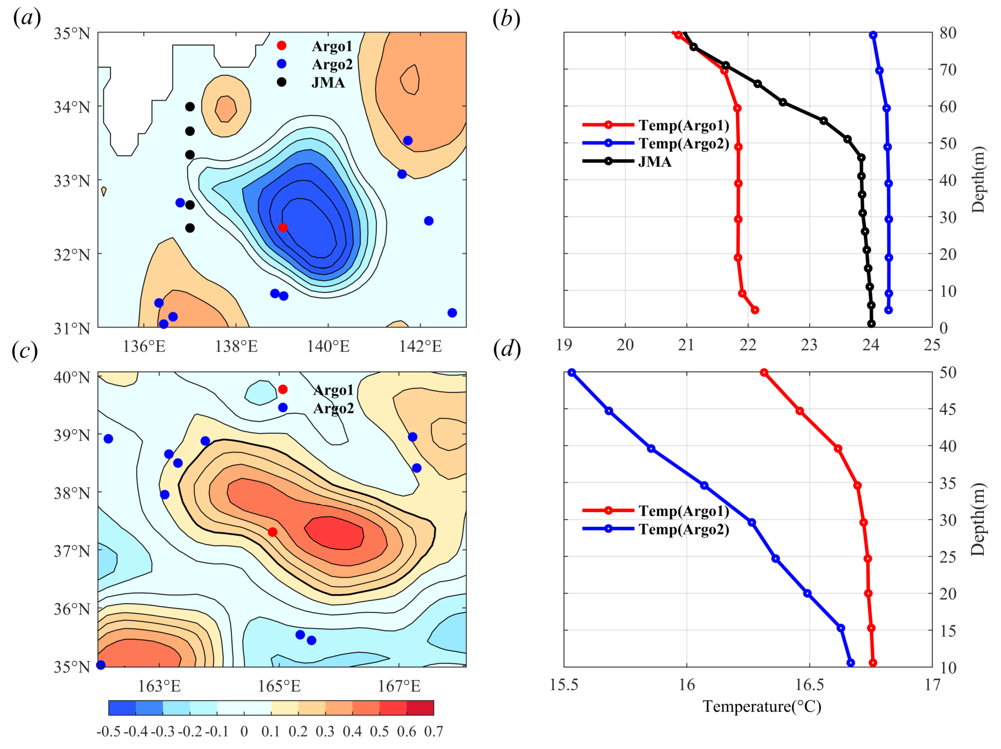
2.1. Data

The data used for identifying the merging of mesoscale eddies originate from the daily sea level anomaly (SLA) fields within the multi-parameter eddy dataset provided by Dong et al. [32]. The SLA fields are established in the “all-satellite” daily Delayed Time (DT) Data Unification and Altimeter Combination System (DUACS) version of 2018. The temporal resolution of 1 day and a spatial resolution of $1/4°$ are sufficient for capturing comprehensive information regarding the merging of mesoscale ocean eddies. Following linear interpolation (to improve the performance of the eddy detection algorithm) by Dong et al. [32], the daily SLA fields are extended to encompass a larger number of grid points, resulting in a grid spacing of $1/6°\times 1/6°$. A geostrophic equilibrium equation is used to determine the latitudinal ($u^{\prime }$) and longitudinal ($v^{\prime }$) velocity components from SLA.

$$u^{\prime }=-\frac{g}{f}\frac{\partial \left(SLA\right)}{\partial y},v^{\prime }=\frac{g}{f}\frac{\partial \left(SLA\right)}{\partial x}$$

(1)

where g represents the gravitational acceleration, $x,y$ are the eastward and northward distances, respectively, and f is the Coriolis parameter.

The SST data are based on AVHRR high-resolution datasets provided by NOAA (National Oceanic and Atmospheric Administration). The spatial resolution is 4 km and the temporal resolution is 1 day. Furthermore, Argo data [33] and shipborne observations along the 137°E meridian by the Japan Meteorological Agency (JMA) [34] have been employed for the analysis of vertical temperature differences within and outside merging eddies. Real-time data from Argo floats are accessible at https://argo.ucsd.edu/ (accessed on 28 August 2023). JMA has been conducting winter observations since 1967 and summer hydrographic observations since 1972 in the western North Pacific along the 137°E meridian, within the range of 3°N–34°N. These shipborne observational datasets are available at https://www.jma.go.jp/ (accessed on 28 August 2023).

2.2. Study Area and Merging Identification Algorithm

The region selected for the current eddy merging cases is the Kuroshio Extension area (about 30°N to 40°N, 130°E to 165°E) in the Subtropical Northwest Pacific. Through satellite observations, this area has been identified to exhibit high eddy variability and is renowned for its intense eddy activity and elevated eddy kinetic energy [35]. Eddies within the Kuroshio Extension area primarily arise due to horizontal barotropic instability and the meandering trajectory of the Kuroshio [36], resulting in a concentrated and densely distributed population of eddies characterized by extended lifespans and substantial dimensions. Given the high frequency of mesoscale eddy activity and significant eddy–eddy interactions within the Kuroshio Extension area, it becomes a pertinent choice for studying eddy merging phenomena.

Due to the oceanic mesoscale, eddies can often be identified as areas surrounded by the closed SLA contours [28,29,37]. Figure 1 displays the distribution of mesoscale eddies in the Kuroshio Extension region, based on sea surface height anomaly data provided by Dong et al. [32]. The colors (arrows) indicate SLA (geostrophic current velocity), with the data recorded on 19 January 2010. From Figure 1, the spatial distribution of SLA effectively illustrates the distinct mesoscale eddy distribution characteristics. And the peripheral SLA enclosed contours of each eddy can also serve as a representation of its intrinsic boundary. For different eddy polarities, cyclones (anticyclones) are characterized by a negative (positive) SLA signal. Furthermore, interactions occur between eddies of opposite polarities, but the boundaries of these eddies do not come into compatibility (Figure 1, purple rectangle). In contrast, eddies of the same polarity can coexist within the same enclosed SLA curves, showcasing the presence of multi-core eddies (Figure 1, orange rectangle). Significantly, as emphasized by Cui et al. [28], the existence of multi-core eddy structures does not definitively point toward eddy merging. It may lead to splitting or maintain an intermediate state between splitting and merging. However, for the merging of two eddies of the same polarity, the multi-core eddy structure becomes the exclusive pathway, as it necessitates the fusion of eddy boundaries.

Many scholars have used and improved the SLA-based approach for extracting information on eddy position and shape [29,38]. This paper proposes the definition of boundaries and centers in the mesoscale eddy merging process, including the single and multi-core eddies.

The definition of single-core eddy parameters is as follows:

• Only one SLA peak exists, defined as the center of the eddy;
• Traversing the entire SLA distribution at 0.02 m intervals outwards from the center, with the outermost SLA contour defined as the eddy boundary, and all internal SLA values should be greater (lower) than the SLA value on the outermost closed contour of the anticyclone (cyclone);
• The amplitude $A>3$ cm, where $A=|a_c-a_b|$, $a_c$ is the SLA for eddy center, $a_b$ is the SLA for eddy boundary. The number of grid points within the eddy boundary should satisfy the following: 20 pixel < Area < 2000 pixel. Due to the launch of the Jason series of altimeters, the minimum amplitude of the eddy is selected from 1 cm [35] to 3 cm [20], which has optimal performance in observations of ocean dynamics.

The definition of multi-core eddy parameters is as follows:

• The outermost closed SLA contour of the eddy is defined as the eddy boundary;
• Multiple local SLA peaks exist;
• The amplitude $A>3$ cm;
• The lifespan of the multi-core eddy is determined by whether one of the interacting eddies dissipates.

3. Results

A large number of mesoscale eddy merging events have occurred in the Kuroshio Extension area. In order to clarify these phenomena and to visualize the implications of their dynamics for studies related to eddy lifetimes, dynamics, and morphology, this section provides an in-depth analysis of the merging events based on satellite altimeter data, using the merging algorithm to extract eddy parameters.

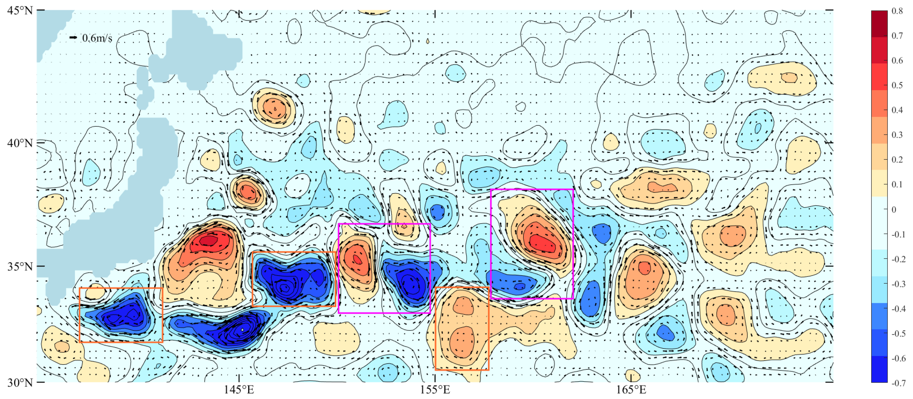
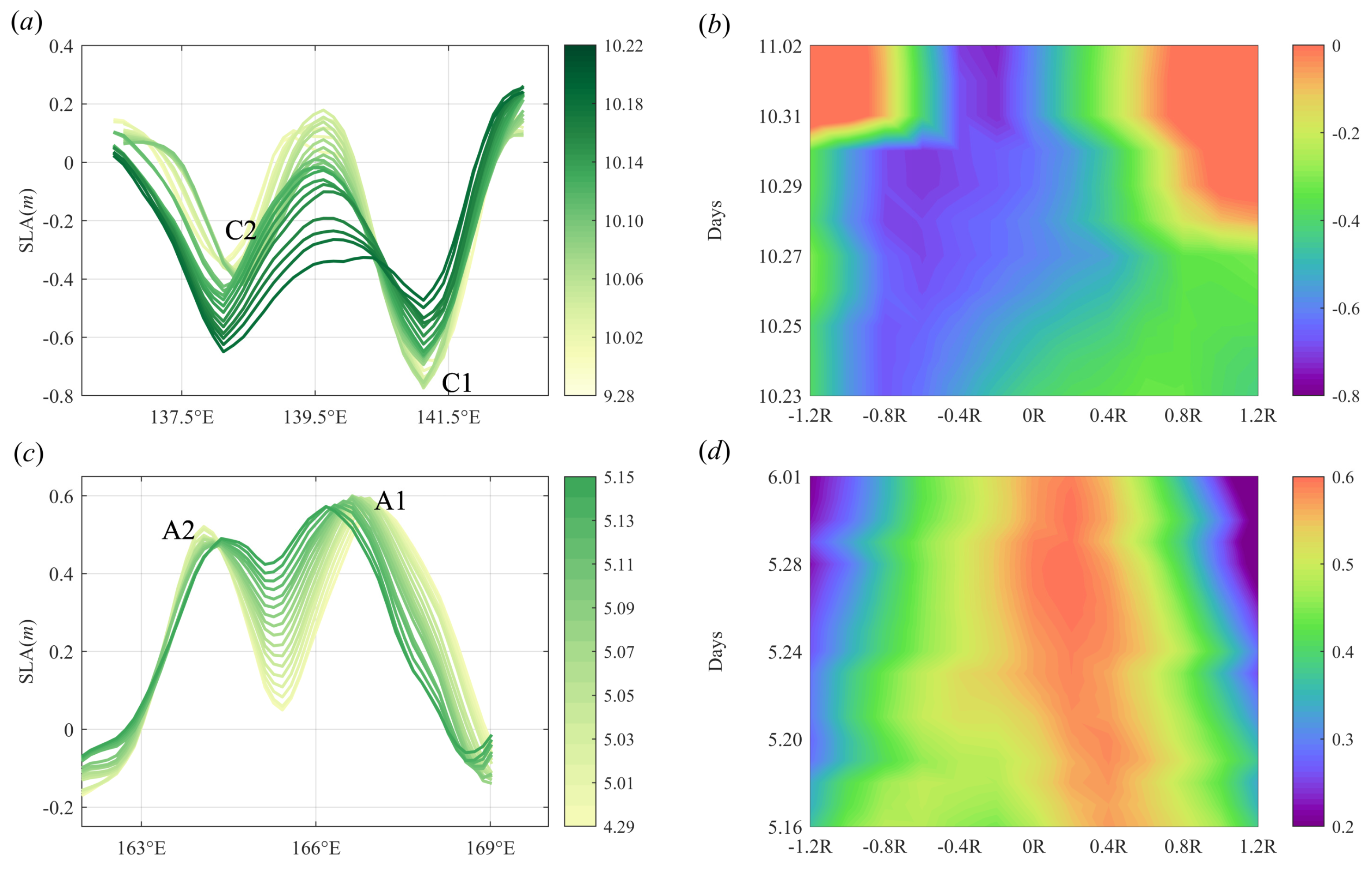
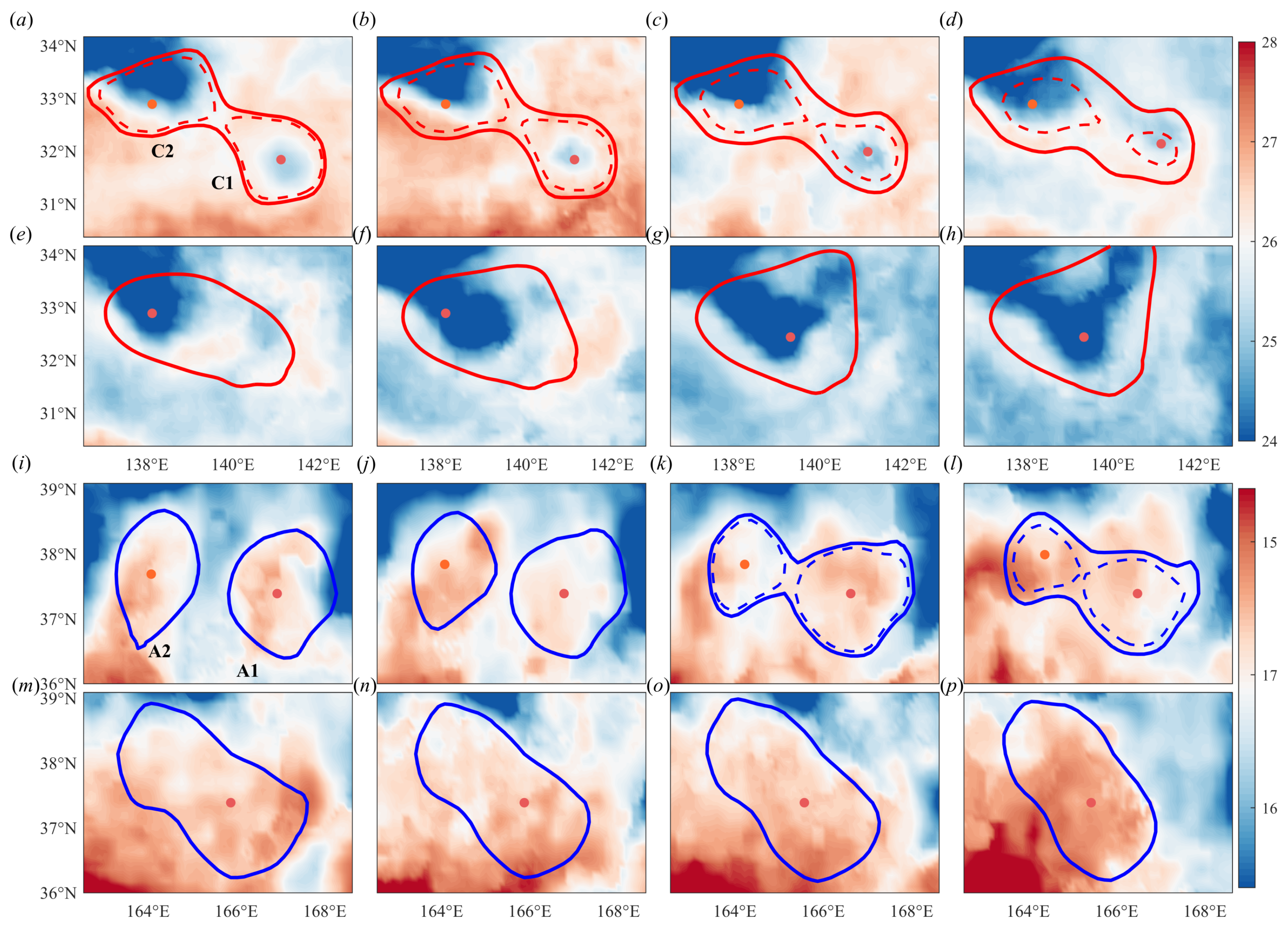
3.1. The Merging Processes

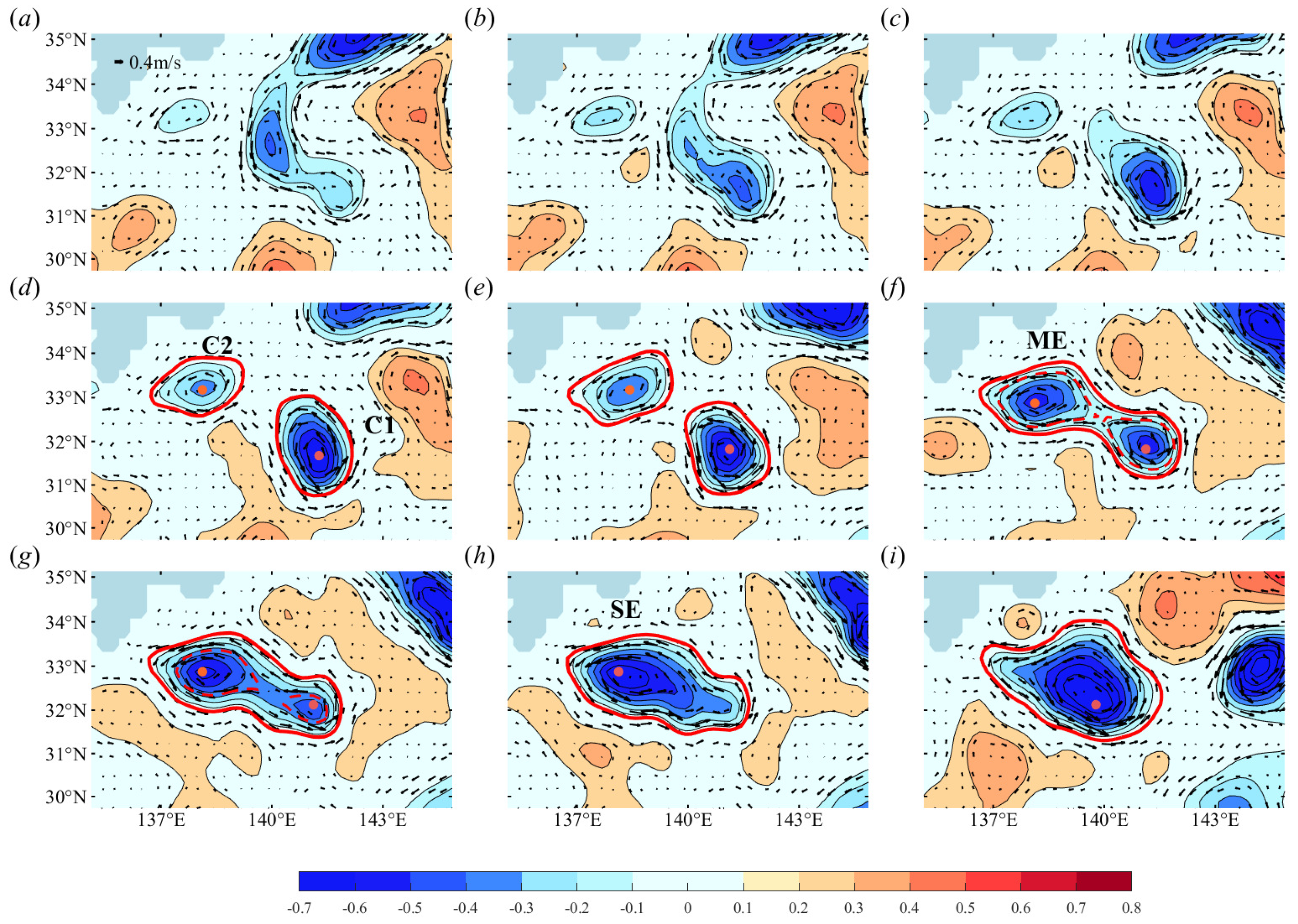
3.1.1. The Merging of Cyclonic Eddies

The merging of two mesoscale cyclonic eddies (137°E–143°E, 30°N–34°N, September–November 2008) is found and monitored by using daily SLA data (Figure 2). The solid red line (solid orange dots) indicates the eddy boundaries (centers) extracted by the merging algorithm in Section 2, C1 and C2 denote two single-core cyclonic eddies, respectively, ME denotes the multi-core eddy structure during the merging, and SE denotes the final generated single-core eddy.

Prior to extracting eddy parameters, Figure 2a–c illustrates the sources and primary movement paths of the eddies. C1 originates from the bifurcation of a cyclone at 143°E, 35°N, while C2 is consistently influenced by the terrain in the northwest direction, forming and stabilizing at 137°E, 33°N. Panels (d-i) in Figure 2 document the complete merging process and showcase the key parameters (boundaries, centers) of the eddies. Initially, before the merging, C1 and C2 are situated in close proximity to one another, maintaining a relatively stable morphology and area (Figure 2d,e). Subsequently, shared contours emerge, encompassing both C1 and C2 within closed SLA contours. A noticeable reduction in the area of C1 becomes evident, accompanied by a gradual elongation of both C1 and C2 along the centerline. During this stage, the eddy exhibited a multi-core structure (ME, Figure 2f,g). As the area of C1 gradually diminished, eventually reaching the predetermined minimum threshold set by the merging algorithm (Area < 20 pixels), C1 dissipated, leading the eddy to revert back to a single-core state (SE, Figure 2h). The boundaries of SE gradually regained their characteristic elliptical configuration, and the center of SE steadily converged toward the geometric center (Figure 2h,i).

In the spatial and temporal distribution of vorticity ($\zeta =\partial v/\partial x-\partial u/\partial y$, Figure 3), there is no association between C1 and C2 in terms of vorticity at the outset (Figure 3a–e). Upon the establishment of shared contours between C1 and C2, a distinct vorticity exchange becomes manifest (Figure 3f). Furthermore, ME and SE display pronounced vorticity distribution within their interiors (Figure 3g–i). The vorticity variability depicted in Figure 3 harmoniously corresponds with the merging process depicted in Figure 2.

Figure 2 and Figure 3 collectively highlight the significance of the multi-core eddy structure and shared contours during eddy merging. To analyze this characteristic, Figure 4a,b magnify the SLA contours distribution of C1 and C2. Furthermore, the average velocity along each enclosed SLA contour $\langle V\rangle$ and its corresponding radius R ($R=\sqrt{S/\pi }$, S indicates the area within the SLA contour) are depicted in Figure 4c,d. The black solid (dashed) line indicates the boundaries of C1 (C2) and the gray thin (thick) solid line indicates the shared contours. It can be found that parts of the SLA contours of C1 and C2 intermingle with each other and gradually enclose them and extend outwards (Figure 4a,b). The magnitude of $\langle V\rangle$ within the shared contours may be greater than that of one or both boundaries of C1 and C2 (Figure 4c,d). This phenomenon suggests that there is a significant interaction between C1 and C2 in the multi-core eddy structure and that it involves an exchange of energy or momentum. Specifically, the interaction between C1 and C2 results in an energy transfer to other regions through the shared contours, leading to an increase in the average velocity along the shared contours compared to the boundaries of C1 and C2. When such shared contours are detected, significant interactions between the eddies are deemed to have occurred, indicating the transition to a multi-core eddy stage [39]. Meanwhile, the essence of the merging is the formation of a new eddy structure whose velocity profile eventually returns to the state depicted in Figure 4c.

Consequently, based on the unique presence of shared contours within the multi-core eddy structure during merging, it becomes possible to delineate the merging stages and investigate the energy and vorticity losses between C1 and C2. In order to objectively delineate the different stages of the merging process, Figure 5 shows the time evolution of the amplitude (A), area (S), eddy kinetic energy ($K{e}_{total},K{e}_{total}={\sum }_{i=1}^n\frac{1}{2}{\mathit{v}}^2$, i denotes the grid point inside the eddy), and vorticity (${\zeta }_{total},{\zeta }_{total}={\sum }_{i=1}^n{\zeta }_i$). Considering the overall characteristics of the changes in the four physical parameters, we can divide the whole process into three different stages as follows (Figure 5, separated by thin black lines):

Phase 1 (around 28 September to 10 October): The variation in C1 and C2 parameters during this phase is not significant, indicating that no clear interaction between C1 and C2 has occurred and that it is a period of single-eddy evolution (Figure 5a–d).

Phase 2 (around 11 October to 23 October): The variation in C1 parameters is very pronounced during this phase, which is a period of eddy-eddy interactions. Until 23 October, the amplitude (area, eddy kinetic energy and eddy vorticity) of C1 is about 0.08 m (0.6 $\times {10}^4$ km², 3.78 m²·s⁻² and 0.88 × ${10}^{-3}$ s⁻²), which is 21.3% (14.5%, 0.06% and 36.8%) of the initial (defined as October 10th as the initial moment of eddy–eddy interaction) amplitude (radius, eddy kinetic energy, and eddy vorticity) (Figure 5a–d). Conversely, the C2 parameter does not vary significantly. Therefore, C2 seems to play a dominant role in the eddy pair, influencing the extinction of C1 (Figure 5a–d).

Phase 3 (around 24 October to 17 November): This phase belongs to the period of merging eddy. Until 24 October, the amplitude (area, eddy kinetic energy, and eddy vorticity) of SE has increased by 33.9% (200%, 250%, and 52.6%) compared to the pre-merging Sum (C1 + C2) on 23 October. Importantly, it can be found that the transition from ME to SE is a continuous process. Taking into account the existence of multi-core eddies, the energy and vorticity balance is maintained before and after the merging. The energy and vorticity lost by C1 and C2 are stored in the shared contour region (Figure 5a–d).

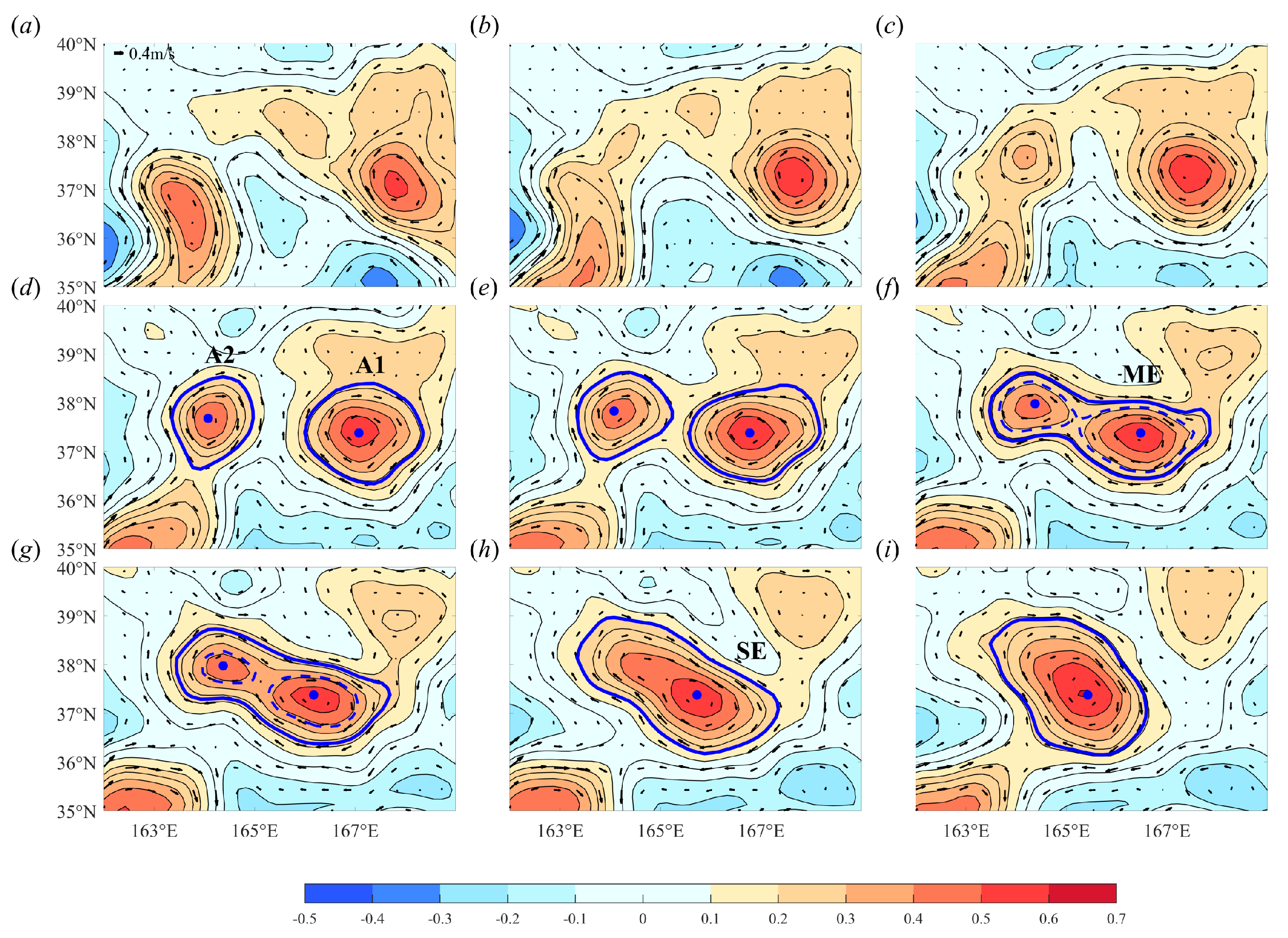
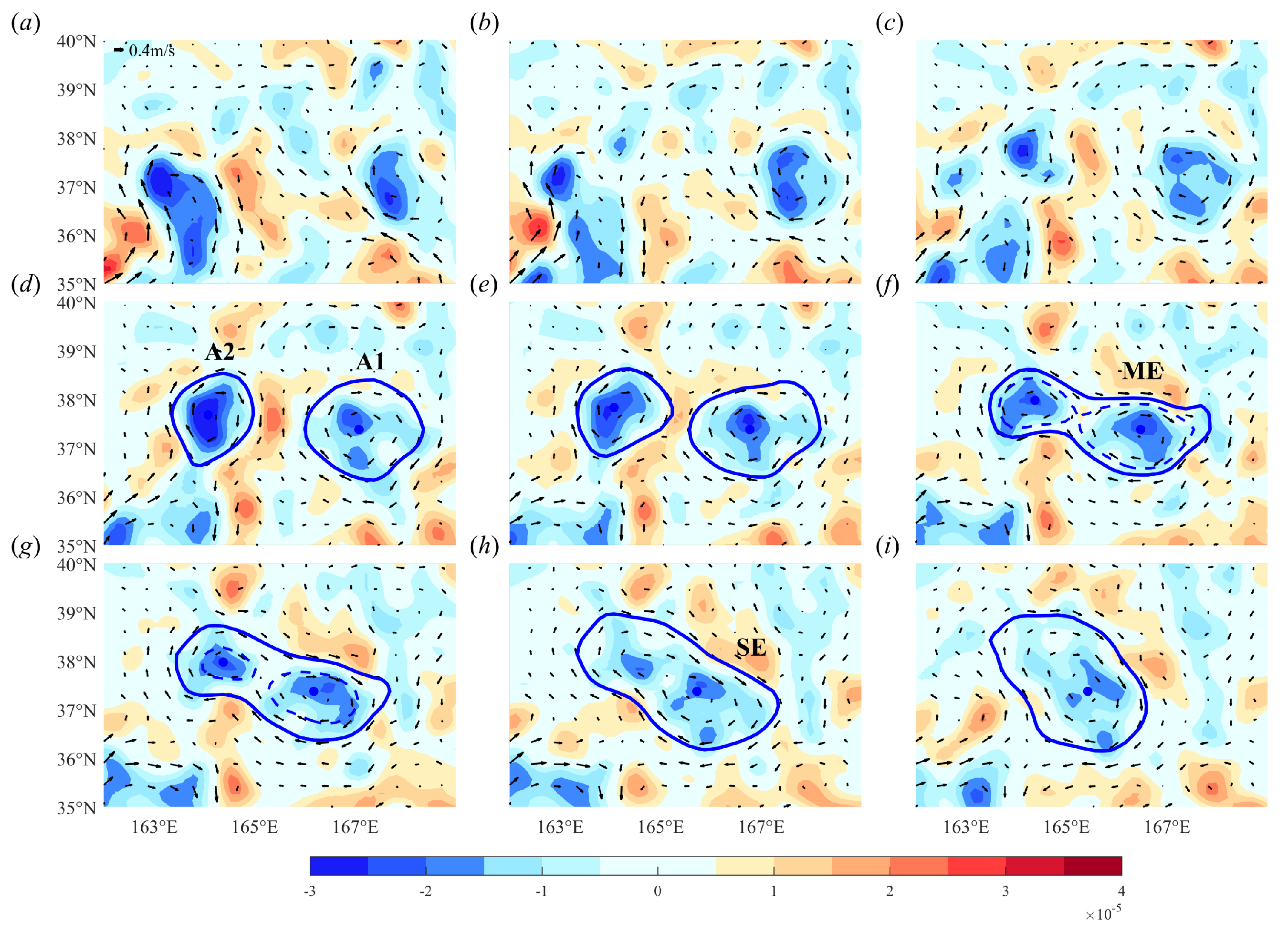
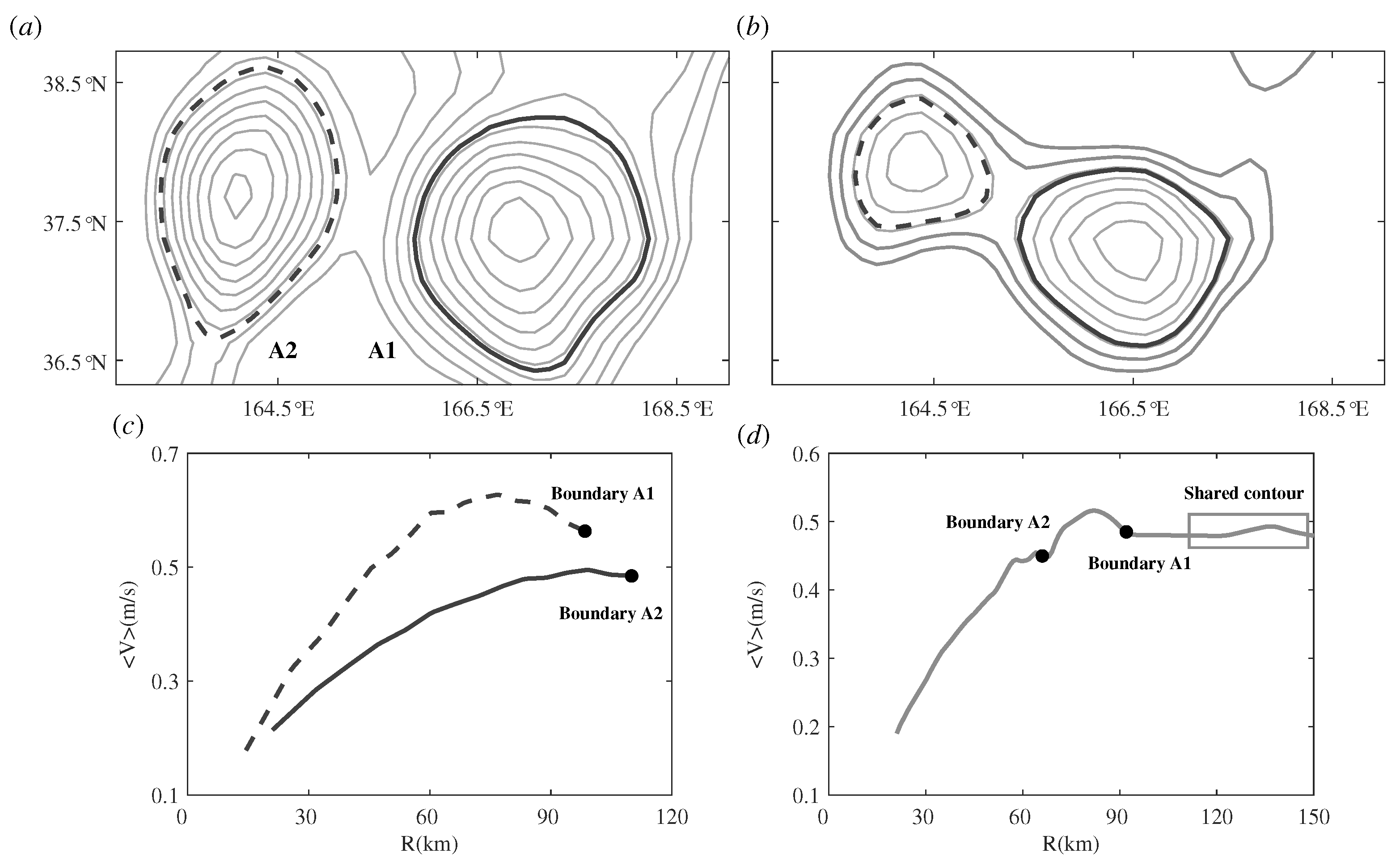
3.1.2. The Merging of Anticyclonic Eddies

The merging of two mesoscale anticyclonic eddies (162°E–169°E, 35°N–40°N) is found and monitored by using daily SLA data (Figure 6). The solid blue line (solid blue dots) indicates the eddy boundaries (centers), while A1 and A2 denote two single-core anticyclonic eddies, respectively.

Before extracting eddy parameters, Figure 6a–c displays the primary sources and movement trajectories of the eddies. A1 sustains a continuous westward motion, while A2 originates from the splitting of an anticyclone positioned at 164°E, 36°N. Panels (d-i) of Figure 6 document the entire merging process and showcase the principal parameters (boundaries, centers) of the eddies. Mirroring the cyclonic eddy merging phenomenon (Figure 2), A1 and A2 also undergo a comparable merging process, involving the establishment of shared contours and the formation of a multi-core eddy structure. (Figure 6). Furthermore, significant vorticity exchange occurs between A1 and A2 (Figure 7f,g), with a more pronounced distribution of negative vorticity within the boundaries of both the ME and SE (Figure 7h,i).

From Figure 8, the average velocity $\langle V\rangle$ within their shared contours still exceed those of one or both boundaries of A1 and A2 (Figure 8c,d). These findings are consistent with the characteristics of the cyclonic eddy merging process (Figure 4).

The variation in the physical parameters during anticyclonic eddy merging is given in Figure 9, with the stages divided as follows:

Phase 1 (around 29 April to 8 May): A period of single-eddy evolution (Figure 9a–d).

Phase 2 (around 9 May to 15 May): The variation in A1 and A2 parameters is very pronounced during this phase, which is a period of eddy–eddy interactions. Until 15 May, the amplitude (area, eddy kinetic energy, and eddy vorticity) of A1 is 39.0% (36.4%, 18.2%, and 55.2%) of the initial (defined as 8 May as the initial moment of eddy–eddy interaction) amplitude (area, eddy kinetic energy, and eddy vorticity), the amplitude (area, eddy kinetic energy, and eddy vorticity) of A2 is 22.4% (24.7%, 0.07%, and 29.1%) of the initial amplitude (area, eddy kinetic energy, and eddy vorticity) (Figure 9a–d). Although A1 and A2 interact with each other during the merging process, A2 is more dramatically affected.

Phase 3 (around 16 May to 29 May): This phase belongs to the period of merging eddy. Until 16 May, the amplitude (area, eddy kinetic energy, and eddy vorticity) of SE has increased by 94.7% (275.4%, 700.3%, and 114.0%) compared to the pre-merging Sum (A1 + A2) on 15 May. However, the transition from ME to SE remains natural and continuous, further indicating that, considering ME and SE, there is a balance in energy and vorticity, and the energy and vorticity lost by A1 and A2 is stored in the shared contour region (Figure 9a–d).

The merging of cyclonic eddies exhibits remarkable similarities to the merging of anticyclonic eddies. Initially, C1 (A1) and C2 (A2) are individually in a period of single-eddy evolution. As the distance between them gradually decreases, the shared contours and multi-core eddy structure are formed. This process is accompanied by significant interactions between the eddies, ultimately resulting in the emergence of a merging eddy. It is important to note that the multi-core eddy structure serves as a critical transitional stage in the eddy merging process, as it embodies the significant interactions between eddies and retains the energy and vorticity that they lose.

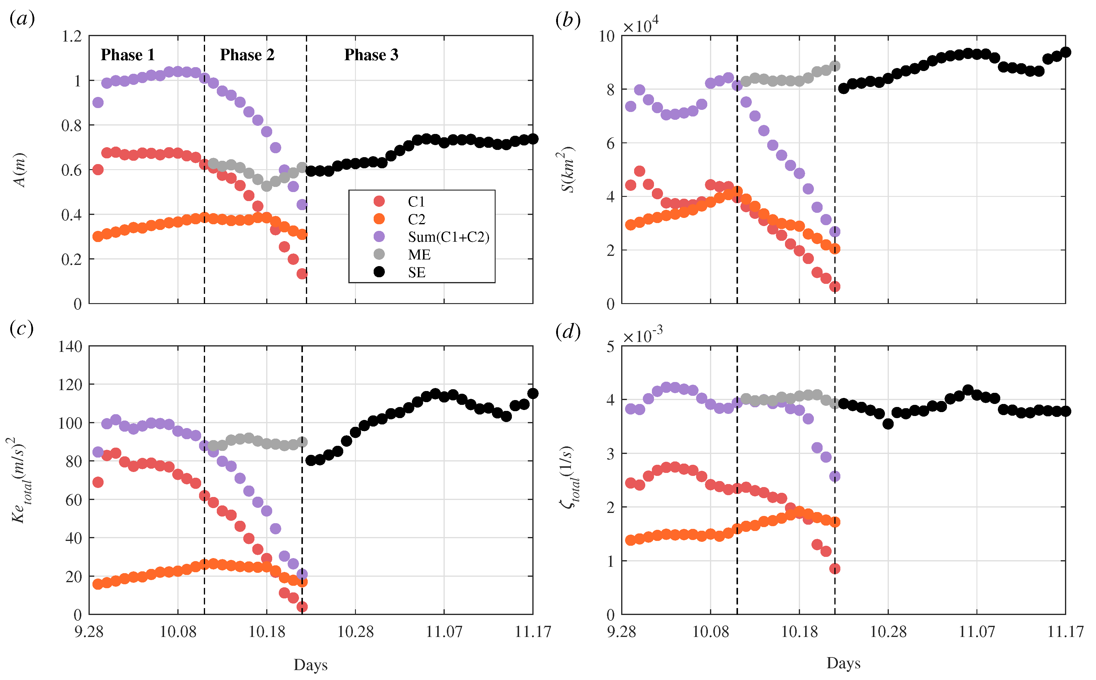
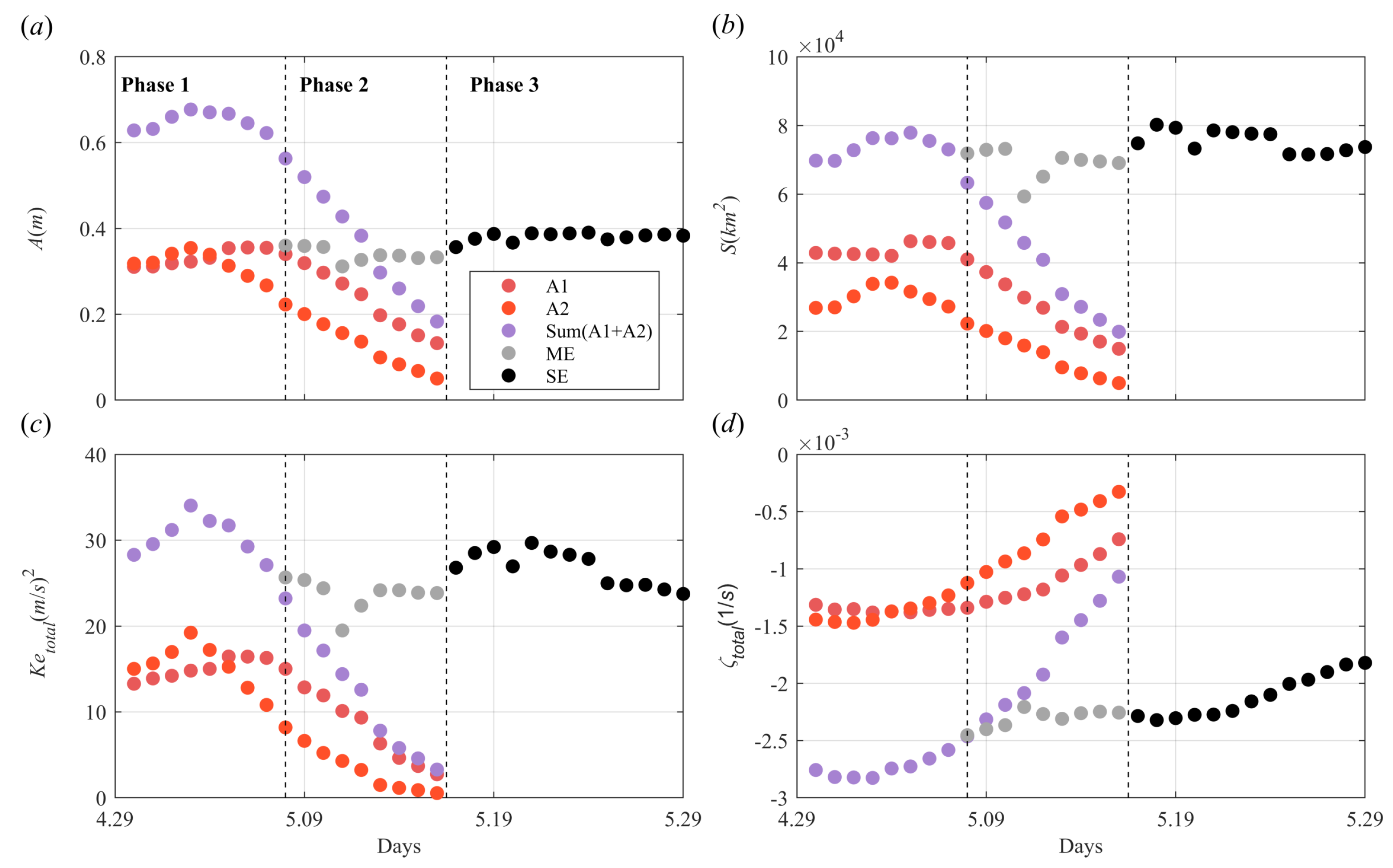
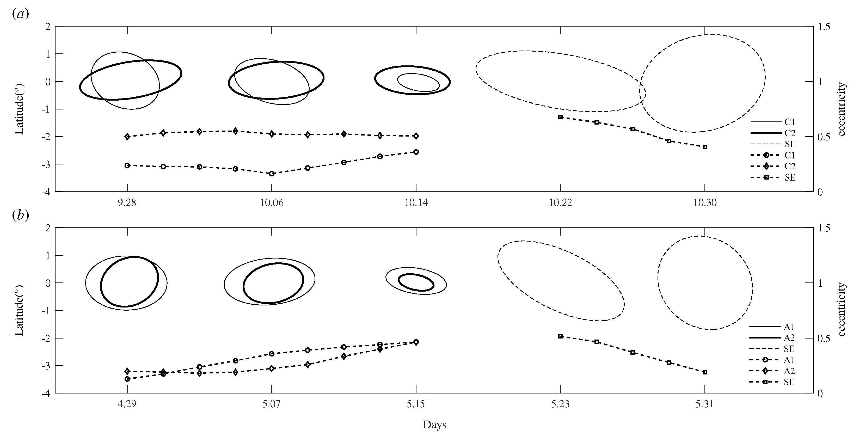
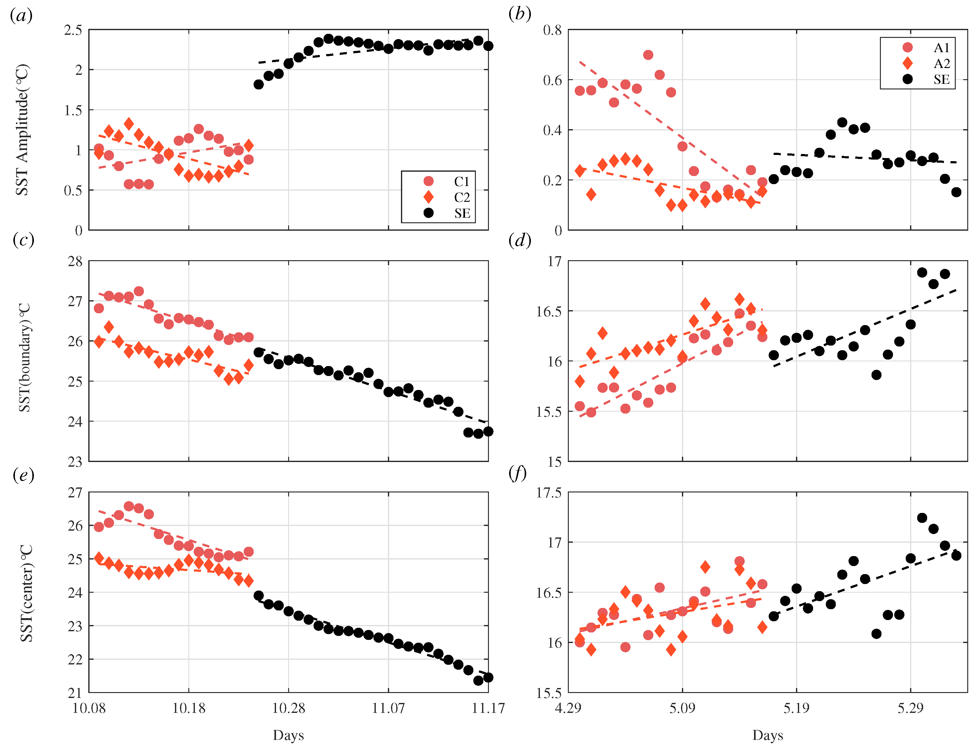
3.2. Morphological Evolution during the Eddy Merging

In addition to the parameters shown in Figure 5 and Figure 9, changes in eddy morphology are also significant indicators of eddy merging. Figure 10 illustrates the morphological evolution of C1 (A1) and C2 (A2) in the horizontal direction during the merging process. Following ellipse fitting, the eccentricity ($(a-b)/a$, where a represents the semi-major axis and b represents the semi-minor axis of the ellipse) of C1 (A1) and C2 (A2) does not exhibit significant changes, while the semi-major axes of C1 (A1) and C2 (A2) stretch in different directions during Phase 1. However, in Phase 2, the stretching directions of C1 (A1) and C2 (A2) gradually align due to eddy–eddy interactions. Ultimately, SE maintains an elongated elliptical structure, inheriting the stretching orientation of C1 (A1) and C2 (A2) prior to merging. This is followed by a continuous decrease in eccentricity, indicating the completion of structural remodeling in Phase 3.

In order to describe the morphological changes of C1 (A1) and C2 (A2) in the vertical direction, we construct profiles of the SLA along the centerline during the merging process (Figure 11a,c). Additionally, radial profiles are obtained within SE along the line connecting the geometric center and the center of the SLA peak (Figure 11b,d). From Figure 11a,c, C1 (A1) and C2 (A2) initially form a distinct double valley (peak) structure on the sea surface, followed by an evolution to a single valley (peak) structure. The magnitude of the SLA change between the eddy centers is most pronounced as C1 (A1) and C2 (A2) gradually approach each other. Eventually, C1 (A2) becomes part of the SLA profile of C2 (A1). Initially, in Phase 3, the peak signal of SLA is around 0.8R (Figure 11b) and 0.4R (Figure 11d) from the geometric center in SE, respectively. Approximately 8 days later, the peak signal of SLAs within cyclonic SE and anticyclonic SE approach their geometric centers around 30 October (Figure 11b) and 24 May (Figure 11d), signifying the completion of both horizontal and vertical structural remodeling.

4. Discussion

It is well-established that the vertical movement of eddies not only facilitates the exchange of seawater but also plays a vital role in the transfer of energy, heat, and matter. Typically, the bottom-up (top-down) motion of seawater at the center of a cyclonic (anticyclonic) eddy induces the dispersion (convergence) of the surrounding water column, resulting in the formation of a cold (warm) eddy. Therefore, the eddy merging process based on sea level anomalies (SLAs) can be validated by employing sea surface temperature (SST) as a tracer. Figure 12 shows the spatial and temporal evolution of the SST during cyclonic and anticyclonic eddies merging. Although the SST data contain a large number of small-scale ocean signals, regions of locally lower (higher) SST than the ambient SST serve as reliable indicators of the locations of mesoscale cyclonic (anticyclonic) eddies (Figure 12a,i). Due to the merging process taking approximately one month, the influence of seasonal climate variations is not significant. From the variation process of SST with eddy merging in Figure 12, it can be found that there are barriers of abnormally high (low) temperature regions between C1 (A1) and C2 (A2). Subsequently, the merging process causes the accumulation of seawater at the intermediate position between C1 (A1) and C2 (A2), leading to the formation of a significant negative (positive) SLAs, as depicted in Figure 11a,c. Consequently, the anomalously cold (warm) regions gradually connect and integrate, as depicted in Figure 12d,l, resulting in the ultimate formation of a single cold (warm) eddy. After the merger, the distribution range of the anomalously cold (warm) regions slowly increases and extends throughout the entire eddy interior, as shown in Figure 12e–h,m–p.

From Figure 12, the spatial distribution of SST within the SE is evident. However, further discussion is needed to explore the physical mechanisms responsible for temperature changes during the eddy merging process. Therefore, Figure 13 displays the temporal evolution of the eddy’s temperature amplitude (SST amplitude, the absolute difference between the SST at the eddy center, and the SST at the eddy boundary). For cyclonic eddy merging, the SST at the newly formed SE boundary closely approximates the average SST of the C1 and C2 boundaries before merging (Figure 13c), while the SST at SE center consistently remains lower than the SSTs of C1 and C2 (Figure 13e). Despite the time-decreasing SSTs at the centers and boundaries of C1, C2, and SE due to the impact of the large-scale background field, the SST amplitude variation at SE significantly increases compared to C1 and C2 (Figure 13a). This phenomenon is likely due to eddy strengthening during merging (enhanced internal SLAs, Figure 11a), leading to cold water upwelling at the eddy center and causing a larger SST amplitude (Figure 13a).

On the other hand, for anticyclonic eddies, the SST at the boundary of the SE is lower than that of A1 and A2 before merging (Figure 13d), while the SST at the center of the SE lies between the SSTs of A1 and A2 (Figure 13f). Despite the time-increasing SSTs at the centers and boundaries of A1, A2, and SE due to the impact of the large-scale background field, the variation in SST amplitude at SE becomes larger compared to A1 and A2 (Figure 13b), indicating an intensified temperature difference between the interior and the boundary of the SE. Unlike cyclonic eddies, anticyclonic eddy merging does not raise the SST at the eddy center (Figure 13f) but lowers the SST at the eddy boundary (Figure 13d). This phenomenon may be attributed to the eddy’s strengthening during merging (enhanced internal SLA, Figure 11a), which induces downward flow and concave isopycnals at the eddy center, while the isopycnals become uplifted at the eddy boundary, leading to a decrease in SST (Figure 13d) and ultimately increasing the SST amplitude.

The SST data provide the distribution of surface temperature before and after the eddy merging, revealing a distinct SST anomaly signal associated with the merging eddy compared to the background field. To further validate this finding and illustrate the vertical profile variations in temperature, we have conducted preliminary analyses using data from Argo floats both within and around the eddy, along with shipborne observations (provided by JMA), as depicted in Figure 14. The temperature profiles from buoys (JMA) surrounding the eddy have been averaged and are displayed in panels b and d of Figure 14. The selected shipborne observation date is 6 November 2008, while the buoys around the eddy are chosen within a 5-day range from the date of the eddy’s center buoy.

The temperature profile collected through shipborne observations exhibit a close correspondence with the temperature profile of buoys encircling the eddy within the vertical range of 0–50 m (Figure 14b). If we liken this concurrence to a baseline state, the merging of the cyclonic eddy results in a pronounced cooling within the eddy’s domain at depths up to 50 m. The merging of the anticyclonic eddy induces a distinct warming across the eddy’s vertical extent (Figure 14d). This conclusion is analogous to the findings presented in Figure 13a,b.

In conclusion, it is found that eddy merging leads to an enhanced SST amplitude within the SE and gradually significant positive (negative) SST anomaly signals. Similar conclusions are drawn from the vertical temperature profiles within the SE’s interior. Nevertheless, due to limited horizonal advection and mixing, the spring/summer (fall/winter) warming (cooling) could lead to higher (lower) SST inside of the eddies than in the surrounding water. This aspect remains unverified by our existing dataset; however, it continues to be a subject of interest for future research. Furthermore, our study encounters formidable challenges, chiefly stemming from the scarcity of vertical data, which impairs our ability to gain a comprehensive understanding of the vertical structure of the merging eddies. To comprehensively reveal the mechanisms behind the SST anomaly signals induced by eddy merging, we are conducting three-dimensional numerical simulations to model and analyze the vertical characteristics of the merging eddies, thus contributing to a deeper understanding of the complex oceanic processes and providing valuable insights for climate and oceanographic research.

5. Conclusions

This study systematically analyzes the merging processes of two case examples involving cyclone–cyclone and anticyclone–anticyclone eddies from the perspective of remote sensing observations by identifying the structure of single/multi-core eddies using the SLA geometric closure profile algorithm.

The merging of eddies in the ocean is typically not the interaction between two equal eddies. The main trend of eddy merging is the absorption of weaker eddies by stronger ones, ultimately forming a larger eddy. The examples of two sets of mesoscale eddy pairs, randomly selected in this study, exemplify the general patterns applicable to eddy merging research. It is found that there are three stages in the merging process: The period of single eddy evolution, eddy–eddy interactions, and the formation of the merging eddy. The process of merging is specified as follows: initially, the eddies are not linked to each other (single eddy evolution); as the distance between the eddies decreases, the shared contours and multi-core eddy structure form, with a significant exchange of energy and vorticity between the two eddies (eddy–eddy interactions), leading to the slow extinction of one of the eddies and the rebirth of the merging eddy (the formation of the merging eddy). Crucially, the multi-core eddy structure and shared contours play a pivotal role as an intermediary phase within the merging process. The areas containing the shared contours gradually absorb the energy and vorticity lost due to the interactions between the two eddy cores. This lost energy and vorticity are then distributed according to the standardized structure of a single eddy. This observation establishes an objective link between the dynamics of the multi-core structure and the energy redistribution occurring within the eddies.

Meanwhile, the eddies have different morphological changes in the horizontal and vertical directions at different stages. Before the formation of the merging eddy, the contours of eddies stretch upwards along the direction of the centerline, and the double-peaked (valley) structure of the SLA gradually evolves into a single-peaked (valley) structure. Following the formation of the merging eddy, the eddy structure grows into a regularized single eddy, and the SLA peak eventually moves toward the geometric center of the merging eddy. Through the analysis of SST variations during the merging process, it is found that local SST values lower (higher) than the surrounding areas still effectively characterize the location of mesoscale cyclonic (anticyclonic) eddies. As the cold (warm) cores approach each other, abnormally low-temperature (high-temperature) regions gradually merge, forming a single cold (warm) core. Furthermore, the newly merging eddies exhibit a more pronounced temperature amplitude and more significant SST anomaly signals compared to the pre-merger state. Furthermore, the use of Argo data and JMA shipborne observation data further demonstrates that the merging of eddies results in a pronounced warming (cooling) along the vertical direction of the eddies.

However, this paper only examines two individual cases of merging between mesoscale eddies, without considering the influence of the surrounding environment (flow, eddies of opposite polarity) on the merging process. Additionally, the study lacks a comparative analysis of the vertical direction flow velocity concerning SST variations. Consequently, some of the research results may not possess significant representativeness. Therefore, a comprehensive investigation into the specific impacts of the surrounding environment on mesoscale eddy merging will be the starting point for future research. Furthermore, it is hoped that a combination of multiple data sources and numerical simulation methods can be employed to further explore the mechanisms of eddy merging processes and their effects on the surrounding environment.

References

- Dong, C.; McWilliams, J.; Liu, Y. Global heat and salt transports by eddy movements. Nat. Commun. 2014, 5, 3294. [Google Scholar] [CrossRef] [PubMed]
- Zhang, Z.; Qiu, B.; Klein, P.; Travis, S. The influence of geostrophic strain on oceanic ageostrophic motion and surface chlorophyll. Nat. Commun. 2019, 10, 2838. [Google Scholar] [CrossRef]
- Sun, W.; Dong, C.; Tan, W.; Liu, Y.; He, Y.; Wang, J. Vertical structure anomalies of oceanic eddies and eddy-induced transports in the South China Sea. Remote Sens. 2018, 10, 795. [Google Scholar] [CrossRef]
- Baltar, F.; Arístegui, J.; Gasol, J. Mesoscale eddies: Hotspots of prokaryotic activity and differential community structure in the ocean. ISME J. 2010, 4, 975–988. [Google Scholar] [CrossRef] [PubMed]
- Braun, C.F.; Gaube, P.; Sinclair, T.; Tane, H.; Skomal, G.B.; Thorrold, S.R. Mesoscale eddies release pelagic sharks from thermal constraints to foraging in the ocean twilight zone. Proc. Natl. Acad. Sci. USA 2019, 116, 17187–17192. [Google Scholar] [CrossRef] [PubMed]
- Morel, Y.; McWilliams, J. Evolution of Isolated Interior Vortices in the Ocean. J. Phys. Oceanogr. 1997, 27, 727–748. [Google Scholar] [CrossRef]
- Sun, W.; Yang, J.; Tan, W.; Zhao, B.; He, Y. Eddy diffusivity and coherent mesoscale eddy analysis in the Southern Ocean. Acta Ocean. Sin. 2021, 40, 1–16. [Google Scholar] [CrossRef]
- Du, Y.; Yi, J.; Wu, D. Mesoscale oceanic eddies in the South China Sea from 1992 to 2012: Evolution processes and statistical analysis. Acta Ocean. Sin. 2014, 33, 36–47. [Google Scholar] [CrossRef]
- Zhang, T.; Li, J.; Xie, L.; Zheng, Q. Statistical Analysis of Mesoscale Eddies Entering the Continental Shelf of the Northern South China Sea. J. Mar. Sci. Eng. 2022, 10, 206. [Google Scholar] [CrossRef]
- Lin, X.; Dong, C.; Chen, D.; Liu, Y. Three-dimensional properties of mesoscale eddies in the South China Sea based on eddy-resolving model output. Deep. Sea Res. Part Oceanogr. Res. Pap. 2015, 99, 46–64. [Google Scholar] [CrossRef]
- Aguedjou, H.M.A.; Chaigneau, A.; Dadou, I. Imprint of Mesoscale Eddies on Air-Sea Interaction in the Tropical Atlantic Ocean. Remote Sens. 2023, 15, 3087. [Google Scholar] [CrossRef]
- Sun, W.; Liu, Y.; Chen, G.; Tan, W.; Lin, X.; Guan, Y. Three-dimensional properties of mesoscale cyclonic warm-core and anticyclonic cold-core eddies in the South China Sea. Acta Ocean. Sin. 2021, 40, 17–29. [Google Scholar] [CrossRef]
- Marez, C.D.; Carton, X.; L’Hegaret, P.; Meunier, T.; Stegner, A. Oceanic vortex mergers are not isolated but influenced by the β-effect and surrounding vortices. Sci. Rep. 2020, 10, 2897. [Google Scholar] [CrossRef]
- Kuo, Y.C.; Chern, C.S. Numerical study on the interactions between a mesoscale eddy and a western boundary current. J. Oceanogr. 2011, 67, 263–272. [Google Scholar] [CrossRef]
- Lamont, T.; Berg, M.A.V.D. Mesoscale eddies influencing the sub-Antarctic Prince Edward Islands Archipelago: Origin, pathways, and characteristics. Cont. Shelf Res. 2020, 210, 104257. [Google Scholar] [CrossRef]
- Cerretelli, C.; Williams, C.H. The physical mechanism for vortex merging. J. Fluid Mech. 2003, 475, 41–77. [Google Scholar] [CrossRef]
- Brandt, L.; Nomura, K. Characterization of the interactions of two unequal co-rotating vortices. J. Fluid Mech. 2010, 646, 233–253. [Google Scholar] [CrossRef]
- Wang, Z.; Sun, L.; Li, Q.; Cheng, H. Two typical merging events of oceanic mesoscale anticyclonic eddies. Ocean Sci. 2019, 15, 1545–1559. [Google Scholar] [CrossRef]
- Ciani, D.; Carton, X.; Verron, J. On the merger of subsurface isolated vortices. Geophys. Astrophys. Fluid Dyn. 2016, 110, 23–49. [Google Scholar] [CrossRef]
- Cui, W.; Yang, J.; Ma, Y. A statistical analysis of mesoscale eddies in the Bay of Bengal from 22-year altimetry data. Acta Oceanol. Sin. 2016, 35, 16–27. [Google Scholar] [CrossRef]
- Leweke, T.; LeDizes, S.; Williamson, C.H.K. Dynamics and instabilities of vortex pairs. Annu. Rev. Fluid Mech. 2016, 48, 507–541. [Google Scholar] [CrossRef]
- Riccardi, G. A complex analysis approach to the motion of uniform vortices. Ocean Dyn. 2018, 68, 273–293. [Google Scholar] [CrossRef]
- Selcuk, C.; Delbende, I.; Rossi, M. Quasiequilibrium states and their time evolution. Phys. Rev. Fluids 2017, 2, 84701. [Google Scholar] [CrossRef]
- Han, G.; Dong, C.; Yang, J. Strain Evolution and Instability of An Anticyclonic Eddy From a Laboratory Experiment. Front. Mar. Sci. 2021, 8, 645531. [Google Scholar] [CrossRef]
- Zhai, X.; Johnson, H.L.; Marshall, D.P. Significant sink of ocean-eddy energy near western boundaries. Nat. Geosci. 2010, 8, 608–612. [Google Scholar] [CrossRef]
- Trodahl, M.; Isachsen, P.E.; Lilly, J.M.; Nilsson, J.; Kristensen, N.M. The regeneration of the Lofoten Vortex through vertical alignment. J. Phys. Oceanogr. 2020, 50, 2689–2711. [Google Scholar] [CrossRef]
- Matsuoka, D.; Araki, F.; Inoue, Y.; Sasaki, H. A New Approach to Ocean Eddy Detection, Tracking, and Event Visualization—Application to the Northwest Pacific Ocean. Procedia Comput. Sci. 2016, 80, 1601–1611. [Google Scholar] [CrossRef]
- Cui, W.; Wang, W.; Zhang, J.; Yang, J. Multicore structures and the splitting and merging of eddies in global oceans from satellite altimeter data. Ocean Sci. 2019, 15, 413–430. [Google Scholar] [CrossRef]
- Tian, F.; Wu, D.; Yuan, L.; Chen, G. Impacts of the efficiencies of identification and tracking algorithms on the statistical properties of global mesoscale eddies using merged altimeter data. Int. J. Remote Sens. 2020, 41, 2835–2860. [Google Scholar] [CrossRef]
- Yi, L.; Du, Y.; He, Z.; Zhou, C. Enhancing the accuracy of automatic eddy detection and the capability of recognizing the multi-core structures from maps of sea level anomaly. Ocean Sci. 2014, 10, 39–48. [Google Scholar] [CrossRef]
- Li, J.; Liang, Y.; Zhang, J. A new automatic oceanic mesoscale eddy detection method using satellite altimeter data based on density clustering. Acta Oceanol. Sin. 2019, 38, 134–141. [Google Scholar] [CrossRef]
- Dong, C.; Liu, L.; Nencioli, F. The near-global ocean mesoscale eddy atmospheric-oceanic-biological interaction observational dataset. Sci. Data 2022, 9, 436. [Google Scholar] [CrossRef] [PubMed]
- Wong, A.P.S. Two Million Temperature-Salinity Profiles and Subsurface Velocity Observations From a Global Array of Profiling Floats. Front. Mar. Sci. 2020, 7, 700. [Google Scholar] [CrossRef]
- Kawakami, Y.; Kojima, A.; Nakano, T.; Murakami, K.; Sugimoto, S. Temporal variations of net Kuroshio transport based on a repeated hydrographic section along 137E. Clim. Dyn. 2022, 59, 1703–1713. [Google Scholar] [CrossRef]
- Qiu, B.; Chen, S. Variability of the kuroshio extension jet, recirculation gyre, and mesoscale eddies on decadal time scales. J. Phys. Oceanogr. 2005, 35, 2090–2103. [Google Scholar] [CrossRef]
- Ji, J.; Dong, C.; Zhang, B.; Liu, Y.; Zou, B.; King, G.P.; Chen, D. Oceanic eddy characteristics and generation mechanisms in the Kuroshio Extension region. J. Geophys. Res. Ocean. 2018, 123, 8548–8567. [Google Scholar] [CrossRef]
- Chelton, D.B.; Schlax, M.G.; Samelson, R.M. Global observations of nonlinear mesoscale eddies. Prog. Oceanogr. 2011, 91, 167–216. [Google Scholar] [CrossRef]
- Lumpkin, R. Global characteristics of coherent vortices from surface drifter trajectories. J. Geophys. Res. Ocean. 2016, 121, 1306–1321. [Google Scholar] [CrossRef]
- Le Vu, B.; Stegner, A.; Arsouze, T. Angular Momentum Eddy Detection and Tracking Algorithm (AMEDA) and Its Application to Coastal Eddy Formations. J. Atmos. Ocean. Technol. 2017, 35, 739–762. [Google Scholar] [CrossRef]
Disclaimer/Publisher’s Note: The statements, opinions and data contained in all publications are solely those of the individual author(s) and contributor(s) and not of MDPI and/or the editor(s). MDPI and/or the editor(s) disclaim responsibility for any injury to people or property resulting from any ideas, methods, instructions or products referred to in the content. |
© 2023 by the authors. Licensee MDPI, Basel, Switzerland. This article is an open access article distributed under the terms and conditions of the Creative Commons Attribution (CC BY) license (https://creativecommons.org/licenses/by/4.0/).
Share and Cite
Fu, M.; Dong, C.; Dong, J.; Sun, W. Analysis of Mesoscale Eddy Merging in the Subtropical Northwest Pacific Using Satellite Remote Sensing Data. Remote Sens. 2023, 15, 4307. https://doi.org/10.3390/rs15174307
Fu M, Dong C, Dong J, Sun W. Analysis of Mesoscale Eddy Merging in the Subtropical Northwest Pacific Using Satellite Remote Sensing Data. Remote Sensing. 2023; 15(17):4307. https://doi.org/10.3390/rs15174307
Chicago/Turabian StyleFu, Minghan, Changming Dong, Jihai Dong, and Wenjin Sun. 2023. "Analysis of Mesoscale Eddy Merging in the Subtropical Northwest Pacific Using Satellite Remote Sensing Data" Remote Sensing 15, no. 17: 4307. https://doi.org/10.3390/rs15174307
APA StyleFu, M., Dong, C., Dong, J., & Sun, W. (2023). Analysis of Mesoscale Eddy Merging in the Subtropical Northwest Pacific Using Satellite Remote Sensing Data. Remote Sensing, 15(17), 4307. https://doi.org/10.3390/rs15174307