The Impact Mechanism of Climate and Vegetation Changes on the Blue and Green Water Flow in the Main Ecosystems of the Hanjiang River Basin, China

Abstract

Water resources management and planning traditionally focus on visible liquid or blue water. However, green water also maintains social development and ecosystem services. Therefore, blue and green water should be incorporated into the watershed management system for evaluating water resources. To analyze the water resources of the Hanjiang River Basin, the SWAT model was set up using long-term and high-precision geographic data. The methods of wavelet analysis and Pearson’s correlation analysis were used to explore the influence mechanism of climate and vegetation changes on the blue and green water flow (BWF and GWF) of the main ecosystems in the basin. The results showed that: (1) The spatial–temporal distribution of the BWF and GWF in the main ecosystems of the basin over the past 50 years was uneven. Forest ecosystems and farmland ecosystems have a greater concentration of water resources in the south, while grassland ecosystems have a greater concentration of water resources in the east. (2) Climate dominates the BWF and GWF changes in the main ecosystems of the basin. The BWF and the precipitation change cycle are synergistic, and the GWF and the temperature change cycle are synergistic. (3) The correlation between vegetation and BWF and GWF in the farmland ecosystem is significant. Vegetation affects the hydrological change process of the BWF and GWF at the microscale. This study can provide data support and scientific rules for ecosystem water resource management in the basin.

1. Introduction

Among the many factors affecting social development, economic development, ecosystem sustainability, and water resources are crucial to ensuring the sustainability of nations, societies, and regions [1]. Water is classified as blue water (BW) or green water (GW) by Falkenmark and Rockström (2006) [2]. Blue water is a visible liquid flow moving on the surface and underground. It is the surface runoff of streams, valleys, and rivers, including underground water storage, to recharge the underground runoff of rivers. Green water is an invisible water vapor entering the atmosphere. It is a vapor/molecular state constrained by molecular forces and driven by thermal effects. Plant (biomass) transpiration is considered productive green water. In contrast, soil evaporation (including interception, puddles, and evaporation from soil water) is considered non-productive green water [3]. Green water is equivalent to the commonly used term, evapotranspiration (E.T.) [4,5]. Usually, water resources are planned and managed based on visible liquid or blue water, while limited research has been conducted on green water [6]. It is important to note that blue water has dominated water perception until recently, representing only one-third of actual freshwater resources today [6,7]. The evapotranspiration of forests, grasslands, wetlands, and farmland returns 65% of the global total precipitation to the atmosphere, thus creating green water [2]. Rivers, lakes, and aquifers store only 35% of precipitation, namely, blue water. Green water is the dominant water resource for agricultural production [7,8]. About 60% of the world’s food production depends on green water, and almost all animal husbandry meat products are produced from green water. At the same time, green water is an important water source to maintain the landscape coordination and balance of terrestrial ecosystems [5]. As well as maintaining the production and service functions of terrestrial ecosystems on Earth, it contributes to solving the problem of water shortages and distribution [9,10]. Therefore, scholars have proposed that green water resources should also be included in the evaluation of water resources such as BW and GW management, BW and GW comprehensive utilization research, natural ecosystems, and food production; green water balanced utilization research should be carried out [4,10] and integrate the BWF and GWF at a higher level, combining land use issues with water resource issues [11].

Much attention has been focused on climate change [12] and vegetation destruction [13,14] caused by human activities worldwide. In particular, global change will affect water resources closely related to human production and life and will occur on multiple spatial and temporal scales [15]. Hydrology and the climate interact, resulting in the complexity, heterogeneity, and uncertainty of vegetation eco-hydrological changes affected by future climate change [16,17], which requires strengthening of the micro-scale study of eco-hydrology for global change [5,18]. Different ecosystems within a watershed perform different soil and water conservation functions, including productivity allocation (energy flow), soil fertility maintenance (nutrient cycling), and hydrological cycle operation [19,20,21]. Despite numerous studies, there are surprisingly few driving mechanisms behind BW and GW changes at the ecosystem scale. To better utilize and manage water resources and allocate the production functions of different ecosystems, it is necessary to reveal the mechanisms by which climate and vegetation changes affect the hydrology of ecosystems from an ecosystem perspective.

After the Pearl River Basin, Hanjiang River Basin is Guangdong Province’s second-largest river basin, serving as a water source for the Hanjiang River Basin and surrounding areas experiencing water shortages. In recent years, water resources have been affected by uneven spatial and temporal changes resulting from global climate change, urbanization, and the changing distribution pattern of BWF and GWF [22,23]. Currently in the Hanjiang River Basin, there have been no studies on the BW and GW in the basin. Among the studies on BW and GW in other basins, Zhang et al. (2020) studied the effects of climate and land use changes on BW and GW in the Ganjiang River Basin [24]. Zang et al. (2019) studied the distribution of green and blue water flows in typical ecosystems in arid basins and a spatiotemporal study of their ecosystem service functions [21]. The impact of climate change on BW and GW has also been studied [25,26]. However, there are fewer studies on the mechanisms of climate and vegetation changes on BW and GW at the ecosystem scale. The upper and middle reaches of the basin are mainly characterized by lush vegetation and diverse species. With the increase of agricultural and industrial development activities, the quality of the ecosystem has decreased, soil erosion is more serious, and the forest ecosystem has degraded [27,28]. To formulate a scientifically sound overall plan for protecting, managing, and developing river basins, the mechanisms of change in BW and GW resources must be studied. Therefore, this paper raises the following scientific questions: (1) What are the spatial–temporal evolution characteristics of BWF and GWF in the main ecosystems of the basin? (2) What is the relationship between climate and vegetation and the BWF and GWF in the main ecosystems? (3) How do climate and vegetation changes affect the BWF and GWF in the main ecosystems of the basin? Based on the Soil and Water Assessment Tool (SWAT) model, this study calculated BWF and GWF at the basin and ecosystem scales. It showed their spatial and temporal distribution characteristics within the main ecosystems of the basin. A second objective is to provide a scientific background and theoretical support for basin water resources management strategy by focusing on how climate and vegetation changes affect basin water resources and ecosystems.

2. Materials and Methods

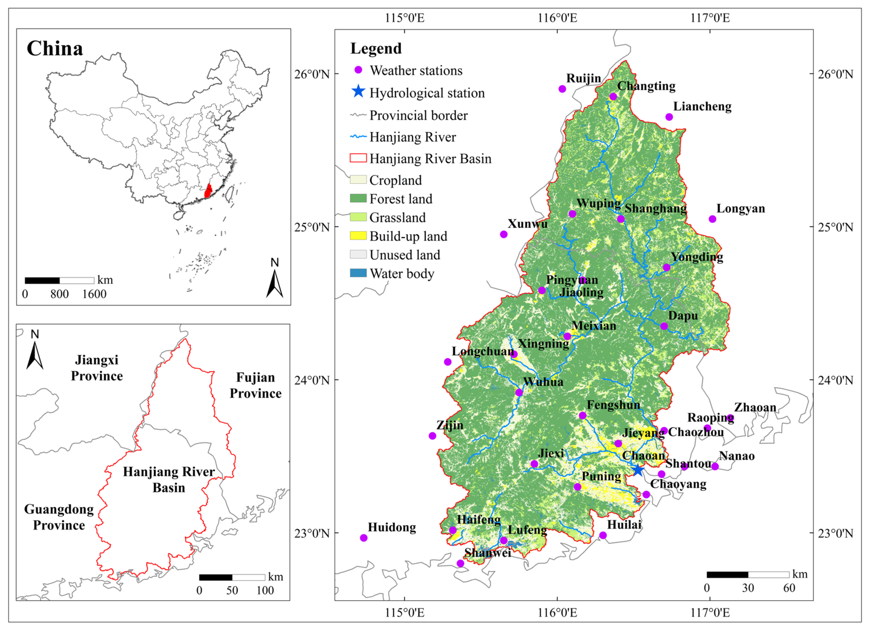
2.1. Research Region

Located at the confluence of the Meijiang River and the Tingjiang River, the Hanjiang River Basin is formed. The Meijiang River originates from the upper peak of Zijin County, Guangdong Province, and runs southwest–northeast. Flowing from north to south, the Tingjiang River originates at Laijia Mountain in Ninghua County, Fujian Province. Hanjiang River was formed by the confluence of the Meijiang River and the Tingjiang River in Dapu County, Meizhou City, Guangdong Province. The middle and upper reaches have sparse populations, while the lower reaches and deltas have dense populations, with Shantou City having the highest density. The basin area is 30,112 km², the mainstream length is 470 km, and the annual runoff is 24.5 billion m³ (Hanjiang River Basin Comprehensive Plan (2021)). Runoff is unevenly distributed, and water resources significantly differ in dry and wet seasons [22]. The basin is greatly affected by the marine Southeast Asian monsoon. During the frost-free season, the temperature is high, the rainfall is plentiful, and the sunshine is sufficient. The average annual precipitation is 1450~2000 mm, and the average annual temperature is 21.4 °C (Hanjiang River Basin Comprehensive Plan (2021)).

Regarding land use types in the basin, forest land accounts for about 67.2% of the area; approximately 18.7% of the land is arable, mainly distributed near the water system; water accounts for about 8.8%; and urban land is about 3.6%, which is concentrated in the southeast of the basin. The grassland area accounts for only about 1.6% (2020) (Hanjiang River Basin Comprehensive Plan (2021)). As the basin rises, the plant resources are vibrant. This region has two types of vegetation: coniferous forests and broad-leaved forests. The middle and lower reaches of the forest consist of broad-leaved evergreens and coniferous mixed forests. Besides tropical evergreen trees, there are also several other tree species with rich biodiversity (Figure 1).

2.2. Materials

A localized SWAT model database was developed using DEM, land uses, soils, meteorological data, and other information collected by the Hanjiang River Basin over the last 50 years.

Table 1. Data information.

Type	Description	Sources
Digital Elevation Model (DEM)	90 m resolution.	Science Data Center of Chinese Academy of Sciences
Land use data	Every decade from 1980 to 2020 (30 m resolution), obtained through remote sensing interpretation.	United States Geological Survey
Soil data	Soil types in China.	Harmonized World Soil Database (HWSD)
Meteorological data	Daily meteorological data of 32 meteorological stations in the Hanjiang River Basin from 1971 to 2020.	National Meteorological Science Data Center of China, Meteorology Bureaus of Guangdong, Fujian and Jiangxi Provinces
Runoff data	Monthly runoff data of Chaoan Station from 1980 to 2010.	Hanjiang River Basin Administration
Vegetation index data (NDVI)	Every five years from 1990 to 2020 (30 m resolution).	Resource and Environment Science and Data Center

shows the sources and specific descriptions of the data. The model used DEM data to generate the river network and delineate sub-basins by developing a vector file of the river network in the basin. Land use, soil, and meteorological data were used to simulate the water resources for the past 50 years. The runoff data were used for model rate calibration and validation. The spatial resolution of land use and NDVI were the same, they were used to analyze the land use and vegetation changes. So, the different spatial resolutions of the data do not affect this study.

2.3. Methods

2.3.1. SWAT Model

The USDA’s Bureau of Agricultural Research developed the watershed-scale SWAT model based on physical-based, deterministic, continuous assumptions [7,29]. The model is widely used worldwide, and its design module is more comprehensive and mature, which can better serve users’ needs [30]. It can be used for research on hydrological conditions and water resource assessment [31], water quality assessment [32], land use change, and environmental impact assessment. Many studies have used this model to simulate and evaluate land use changes and climate change in combination [33]. As such, the SWAT model was chosen to explore the impact of changing conditions on hydrological conditions and to simulate water resource evolution in the basin.

Based on the topography, land, soil conditions, and climate of the basin, the basin’s SWAT model was constructed in this study. The SWAT model’s watershed delineation tool automatically calculates and generates the stream network based on the input DEM. The area thresholds are matched with the actual river network to get the most suitable one. Once the watershed outlets are manually entered, the model automatically generates 48 sub-basins. The water balance equation for the basin is satisfied by the simulated hydrological cycle:

$${SW}_t={SW}_0+\sum _{i=1}^t\left(P_{day}-Q_{surf}-E_a-W_{seep}-Q_{gw}\right),$$

(1)

In the formula, ${SW}_t$ represents the final soil water content (mm); ${SW}_0$ represents the early soil water content (mm); $t$ represents the time step (d); $P_{day}$ represents the precipitation (mm) on the first day; $Q_{surf}$ represents the surface runoff (mm) on day $i$; $E_a$ represents the evapotranspiration on day $i$ (mm); $W_{seep}$ represents the soil infiltration and lateral flow (mm) on day $i$; and $Q_{gw}$ represents the amount of water in return flows (mm) on day $i$.

2.3.2. The Calibration and Verification of the Model

The SWAT model was calibrated and verified using the monthly runoff data from the Chaoan hydrological station. The SUFI-2 (Sequential Uncertainty Fitting Process, version 2) method in SWAT-CUP was used to analyze and calibrate the parameter sensitivity. The accuracy of the model was evaluated by the Nash coefficient ($E_{ns}$) and determination coefficient ($R^2$). The calculation formulas of $R^2$ and $E_{ns}$ are as follows:

$$R^2=\frac{{\left[{\sum }_{i=1}^n\left(Q_{Oi}-\overline{Q_O}\right)\left(Q_{mi}-\overline{Q_m}\right)\right]}^2}{{\sum }_{i=1}^n{\left(Q_{Oi}-\overline{Q_O}\right)}^2{\sum }_{i=1}^n{\left(Q_{mi}-\overline{Q_m}\right)}^2},$$

(2)

$$E_{ns}=1-\frac{{\sum _{i=1}^n\left(Q_{mi}-Q_{Oi}\right)}^2}{\sum _{i=1}^n\left(Q_{Oi}-\overline{Q_O}\right)},$$

(3)

In the formula, $Q_{mi}$ represents a simulated runoff sequence; $Q_{Oi}$ represents the measured runoff sequence; $\overline{Q_O}$ represents the arithmetic mean value of the measured runoff series; $\overline{Q_m}$ represents the arithmetic mean value of the simulated runoff series; and $n$ represents the number of simulation periods.

The values of $R^2$ and $E_{ns}$ range from 0 to 1. Models have a better effect when the value is close to 1. In the existing studies using the SWAT model, the calibration and verification results of the SWAT model are mostly between 0.7 and 0.85. The calibration and verification results of the SWAT model established by this study’s five phases of land use are higher than 0.9 (

Table 2. SWAT model simulation results of land use in five periods.

Year	Calibration		Verification
	${\mathit{R}}^2$	${\mathit{E}}_{\mathit{n}\mathit{s}}$	${\mathit{R}}^2$	${\mathit{E}}_{\mathit{n}\mathit{s}}$
1980	0.96	0.95	0.92	0.92
1990	0.96	0.93	0.95	0.93
2000	0.96	0.95	0.94	0.94
2010	0.95	0.95	0.94	0.92
2020	0.95	0.94	0.95	0.93

), indicating that the model has high credibility and can meet the research needs.

2.3.3. Calculation of BWF and GWF

Based on the definition and SWAT’s output, blue water flow equals root zone seepage, surface runoff, and lateral flow [7]. Green water flow equals evapotranspiration [7]. The calculation formula is as follows:

$$BWF=\sum _{i=1}^n\left(PERC+SURQ+LATQ\right)\times S_i\times 1000,$$

(4)

$$GWF=\sum _{i=1}^{n}ET\times S_i\times 1000,$$

(5)

In the formula, $BWF$ is blue water flow (m³); $GWF$ is green water flow (m³); $PERC$ represents the amount of root zone seepage (mm) in the time step; $SURQ$ represents the surface runoff (mm) generated in the HRU in the time step; $LATQ$ represents the lateral flow into the river (mm); $ET$ represents the evapotranspiration (mm) in the HRU in the time step; $S_i$ represents the catchment area (km²) of the $i$-th HRU; and $n$ represents the number of hydrological response units.

Change rates in water resources are calculated as follows:

$$∆=\frac{n-m}{m}\times 100\%,$$

(6)

In the formula, $m$ represents the base value and $n$ represents the changed value.

2.3.4. Driving Mechanism Analysis Methods

• Morlet Wavelet Analysis

In time-frequency analysis, wavelets are widely used. Using the wavelet base, it analyzes the information at each scale level of the signal and extracts the frequency and time signals from the data signal. Besides finding the mutation point of the data, it shows the singular information within the data and analyzes it in stages [34]. Its mathematical expression is:

$$W_f\left(a,b\right)={\left|a\right|}^{-\frac{1}{2}}{\int }_{-\infty }^{+\infty }f\left(t\right)\phi \ast \left(\frac{t-b}{a}\right)dt,$$

(7)

In the formula, $W_f\left(a,b\right)$ represents the wavelet coefficient; $a$ represents the scaling factor; $b$ represents a translational factor; $t$ represents time; $f\left(t\right)$ represents an arbitrary square-integrable function, that is, the time series of the research object; $\phi \left(t\right)$ represents an essentialize function; and $\phi \ast \left(t\right)$ represents a conjugate function.

Wavelet contour maps can be used to represent periodic changes and to predict future trends. By using the wavelet variance, we can determine the main period of each scale change. The periodic detection of annual temperature data and BWF and GWF data in the basin in the past 50 years was carried out by wavelet analysis.

2.

Pearson’s Correlation Coefficient

In statistics, the Pearson correlation coefficient measures the linear correlation between two variables, ranging from −1 to 1 [35]. The formula is:

$$r=\frac{\sum _{i=1}^n{X}_i{Y}_i-n\overline{X}\overline{Y}}{\sqrt{\left(\sum _{i=1}^n{X}_i^2-n{\overline{X}}^2)\right(\sum _{i=1}^n{Y}_i^2-n{\overline{Y}}^2)}},$$

(8)

Pearson’s correlation coefficients range from −1 to 1. The value 1 indicates that a linear equation can describe X and Y, that all the data points are straight lines, and that Y increases with increasing X. Y decreases as X increases when a value of −1 is used. The value of 0 indicates that the variables do not correlate linearly.

3.

Land Use Transfer Matrix

The land use transfer matrix derived from quantitative descriptions of the system state and state transfer is an application of the Markov model to land use change [36]. We can measure both the transformation between different types of land use and the rate at which it is transferred.

Table 3. Example of land use transfer matrix.

		${\mathit{T}}_2$				${\mathit{P}}_{\mathit{i}+}$	Decrement
		${\mathit{A}}_1$	${\mathit{A}}_2$	…	${\mathit{A}}_{\mathit{n}}$
$T_1$	$A_1$	$P_{11}$	$P_{12}$	…	$P_{1n}$	$P_{1+}$	$P_{1+}-P_{11}$
	$A_2$	$P_{21}$	$P_{22}$	…	$P_{2n}$	$P_{2+}$	$P_{2+}-P_{22}$
	⋮	⋮	⋮	⋮	⋮	⋮	⋮
	$A_n$	$P_{n1}$	$P_{n2}$	…	$P_{nn}$	$P_{n+}$	$P_{n+}-P_{nn}$
$P_{+j}$		$P_{+1}$	$P_{+2}$	…	$P_{+n}$	1
Increment		$P_{+1}-P_{11}$	$P_{+2}-P_{22}$	…	$P_{+n}-P_{nn}$

shows the matrix example:

In the matrix, the row represents the land use type at time point $T_1$, and the column represents the land use type at time point $T_2$. $P_{ij}$ represents the percentage of the area of land type $i$ converted to land type $j$ in the total land area during $T_1-T_2$; $P_{ii}$ represents the percentage of area where $i$ land use types remain unchanged during $T_1-T_2$. $P_{i+}$ represents the percentage of the total area of the land type $i$ at $T1$. $P_{+j}$ represents the percentage of the total area of $j$ land use types at $T_2$. $P_{i+}-P_{ii}$ is the percentage of area reduction of land type $i$ during $T_1-T_2$; $P_{+j}-P_{ii}$ is the percentage of area increase of land type $j$ during $T_1-T_2$.

3. Results

3.1. Variation in Temporal and Spatial Dimensions of BWF and GWF in Main Ecosystems of the Basin in Recent 50 Years

According to the research results, the basin BWF during the past 50 years averaged 367.90 billion m³, and the GWF averaged 306.43 billion m³. The Hanjiang River Basin Comprehensive Plan (2021) states that the basin’s water resources amount is about 300 billion m³. The average annual evapotranspiration over the years is 959–1248 mm, or 288.77–375.80 billion m³. Considering the error between the model simulation and the actual, the calculation results are within a reasonable range. Forest ecosystems contribute the most water to the overall basin (Figure 2), of which BWF accounts for about 67% and GWF accounts for about 70%. The BWF in the farmland ecosystem accounts for about 21% of the total BWF in the basin, and the GWF accounts for about 20%. The BWF and GWF of the grassland ecosystem accounted for 10% of the entire watershed. The proportion of BWF and GWF in the three ecosystems is about 7:2:1.

From a time perspective, the BWF increased in the basin from 1980, decreased from 1990 to 2010, and then increased again from 2010 to 2020. Contrary to the BWF, the GWF decreased significantly from 1980 to 1990, increased slightly from 1990 to 2010, and increased slightly from 2010 to 2020. Generally, the relationship between the BWF and GWF is ‘reciprocal’, and the sum of the two is conserved. The variation trend of the BWF and GWF in each ecosystem is the same as the total amount of BWF and GWF in the basin.

The spatial distribution characteristics of the BWF and GWF in the forest system of the basin showed a general shift towards the southwest from 1980 to 2020. Between 1980 and 1990, the central and northeastern parts of the basin had a large increase in BWF (Figure 3 and Figure 4). At the same time, the GWF of the forest ecosystem showed a decreasing trend, especially in the northeast and west of the basin. From 1980 to 2000, the BWF in the forest ecosystem of the basin was decreasing, with the largest change in the middle of the basin. Meanwhile, the GWF showed an increasing trend, mainly in the basin’s northern, western, and eastern parts. From 2010 to 2020, the BWF of the forest ecosystem increased while the GWF decreased, but the overall change range of the BWF and GWF was smaller than in the previous 40 years.

The farmland ecosystem and grassland ecosystem have significantly different BWF and GWF characteristics than the forest ecosystem. The BWF and GWF are mainly concentrated in the basin’s south, while they are less concentrated in the middle and north. There is a concentration of BWF and GWF in the eastern part of the basin, especially in the southeastern region. The central and western regions are less distributed, and even the water resources of the grassland ecosystem in some sub-basins are close to zero. Water resources in the grassland ecosystem generally increase from west to east. The spatial variation characteristics of BWF and GWF in the farmland and grassland ecosystems are the same as in the forest ecosystem. The difference is that the growth rate of the BWF in individual sub-basins of the grassland ecosystem was greater than 0 in 1980~2000, and the overall change rate of the BWF in these two periods was less than 0 (Figure 5 and Figure 6).

3.2. Driving Mechanism of BWF and GWF Change

3.2.1. The Correlation between Climate Change and BWF and GWF and Its Driving Mechanism

It was found by wavelet analysis that under the first main cycle (about 56 years), the precipitation, temperature, BWF, and GWF in the basin had obvious change cycles of about 35 years. Under the second main cycle (about 13 years), the period of precipitation and BWF was about 8~10 years, and the periodicity of precipitation and water resources after 2000 is more obvious than that before 2000 (Figure 7). Under the second main cycle, the temperature and GWF had no obvious periodicity, but it can be seen that after 2005, the temperature and GWF began to show a periodic trend (Figure 7 and Figure 8). In general, the wavelet analysis results of BWF are synergistic with precipitation, and the wavelet analysis results of GWF are synergistic with temperature, showing a strong correlation between precipitation change and BWF as well as a strong correlation between temperature change and GWF.

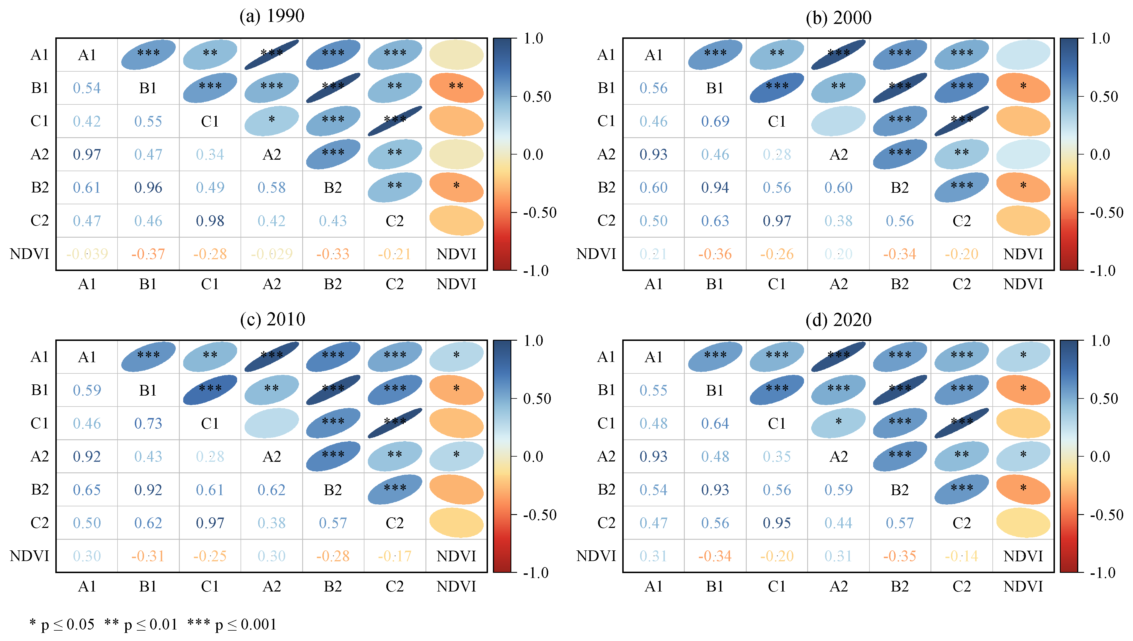
3.2.2. The Correlation between NDVI and BWF and GWF and Its Driving Mechanism

In the research, the NDVI of the basin in the four periods of 1990, 2000, 2010, and 2020 was statistically divided according to the range of 48 sub-basins. The BWF and GWF sequences with a length of 48 in the three main ecosystems of the basin were analyzed with the NDVI sequence for Pearson’s correlation analysis, and the results shown in Figure 9 were obtained. The results showed that the NDVI was significantly correlated with the BWF and GWF in farmland ecosystems in the 1990s. In the 2000s, the NDVI was significantly correlated with the BWF and GWF in farmland ecosystems. Still, the correlation with BWFs decreased from $p \le 0.01$ to $p \le 0.05$. In the decade of the 21st century, the NDVI was significantly correlated with the BWF in the farmland ecosystem as well as the BWF and GWF in the forest ecosystem. In the 1920s, the NDVI significantly correlated with both the BWF and GWF in forests and farmland ecosystems.

The correlation between vegetation and water resources in the main ecosystems in the basin in the past 30 years was as follows: before 2000, the correlation between vegetation and the BWF and GWF in forest ecosystems was not significant, but only with BWF and GWF in farmland ecosystems. However, after 2000, the correlation between the vegetation and the forest ecosystem water resources became significant. The correlation between the vegetation and the BWF and GWF in grassland ecosystem has not been strong (Figure 9).

Figure 10 shows the spatial-temporal evolution of the vegetation index in the basin, which was below 0.5 in 1990 in the western and southern parts. Before 2000, the vegetation index of the basin was very low, mostly between 0.5 and 0.7. After 2000, the vegetation index of the whole basin increased steadily, the area with an NDVI higher than 0.8 increased significantly, and the NDVI of the basin reached its peak in 2015. From 2015 to 2020, the vegetation index of the basin decreased significantly, and the NDVI of a large basin area dropped below 0.8 in 2020. This is because from the 1950s to the 1980s, many large-scale deforestations caused serious damage to forest vegetation (Figure 11). Therefore, in 1985, Guangdong Province proposed “eliminating barren mountains in 5 years and greening Guangdong in 10 years”. All localities vigorously carried out afforestation activities, and the forest ecology of the whole basin was gradually restored and improved. In recent decades, however, the urbanization process in the basin has been evident due to rapid population growth and economic development. Urbanization has occurred on a large scale every decade. Among them, cultivated land converted to urban land mostly before 2000, and cultivated land and forest land converted mostly after 2000 (

Table 4. Land use transfer matrix of the basin.

Area Ratio		1990						Variable Quantity
		CL 1	FL 2	GL 3	W 4	RL 5	UL 6
1980	CL	19.920%	0.024%	0.006%	0.018%	0.381%	0.000%	−0.421%
	FL	0.005%	67.649%	0.007%	0.004%	0.016%	0.003%	0.002%
	GL	0.000%	0.002%	9.115%	0.000%	0.002%	0.000%	0.009%
	W	0.002%	0.001%	0.000%	1.418%	0.001%	0.000%	0.017%
	RL	0.001%	0.000%	0.000%	0.000%	1.393%	0.000%	0.399%
	UL	0.000%	0.002%	0.000%	0.000%	0.000%	0.032%	0.001%
Area Ratio		2000						Variable Quantity
		CL	FL	GL	W	RL	UL
1990	CL	19.322%	0.019%	0.001%	0.003%	0.584%	0.000%	−0.579%
	FL	0.015%	67.599%	0.037%	0.000%	0.025%	0.003%	0.255%
	GL	0.002%	0.275%	8.845%	0.000%	0.006%	0.001%	−0.244%
	W	0.010%	0.000%	0.000%	1.428%	0.001%	0.000%	−0.009%
	RL	0.000%	0.000%	0.000%	0.000%	1.792%	0.000%	0.615%
	UL	0.000%	0.003%	0.001%	0.000%	0.000%	0.031%	−0.001%
Area Ratio		2010						Variable Quantity
		CL	FL	GL	W	RL	UL
2000	CL	18.831%	0.003%	0.000%	0.057%	0.458%	0.000%	−0.494%
	FL	0.022%	67.375%	0.082%	0.068%	0.315%	0.033%	−0.411%
	GL	0.002%	0.025%	8.755%	0.021%	0.081%	0.000%	−0.045%
	W	0.000%	0.000%	0.000%	1.430%	0.001%	0.000%	0.147%
	RL	0.000%	0.000%	0.000%	0.002%	2.405%	0.000%	0.853%
	UL	0.000%	0.000%	0.002%	0.000%	0.000%	0.032%	0.031%
Area Ratio		2020						Variable quantity
		CL	FL	GL	W	RL	UL
2010	CL	18.663%	0.006%	0.001%	0.002%	0.182%	0.000%	−0.182%
	FL	0.007%	67.229%	0.006%	0.007%	0.153%	0.000%	−0.144%
	GL	0.001%	0.008%	8.776%	0.003%	0.051%	0.000%	−0.048%
	W	0.000%	0.003%	0.000%	1.570%	0.004%	0.000%	0.006%
	RL	0.001%	0.006%	0.007%	0.001%	3.246%	0.000%	0.377%
	UL	0.000%	0.000%	0.000%	0.000%	0.003%	0.062%	−0.003%
Area Ratio		2020						Variable quantity
		CL	FL	GL	W	RL	UL
1980	CL	18.610%	0.050%	0.012%	0.076%	1.600%	0.000%	−1.675%
	FL	0.044%	66.887%	0.133%	0.081%	0.499%	0.038%	−0.297%
	GL	0.005%	0.306%	8.642%	0.024%	0.141%	0.001%	−0.328%
	W	0.013%	0.003%	0.001%	1.400%	0.005%	0.000%	0.161%
	RL	0.001%	0.001%	0.001%	0.002%	1.388%	0.000%	2.244%
	UL	0.001%	0.004%	0.003%	0.000%	0.004%	0.023%	0.028%

¹ CL: cultivated land. ² FL: woodland. ³ GL: grassland. ⁴ W: water. ⁵ RL: urban land. ⁶ UL: unused land.

). Although afforestation activities exist in the basin, forest land increased significantly between 1990 and 2000. Between 1980 and 1990, forest land areas barely changed, and between 2000 and 2020, forest land areas were still significantly reduced.

4. Discussion

Over the last 50 years, the land use of the basin has changed. Still, the BWF and GWF distribution patterns in each ecosystem have not significantly changed, thus indicating that land use changes have not significantly affected water resource distribution patterns. The patterns of change in BWF and GWF are very similar in different ecosystems (Figure 10 and Figure 11). That is because climate change dominates water resource changes in both climate change and land use change (including vegetation). The pattern of BW and GW changes among different ecosystems will remain relatively consistent [23]. Nevertheless, drastic changes in local land use patterns have also significantly impacted the BWF and GWF within the small local watershed, affecting the hydrological processes of the water cycle in the watershed, thereby changing the proportion of BWF and GWF in the watershed [20,37,38]. This is reflected in the fact that in the southwestern and northern margins of the basin with low vegetation coverage, the variation in BW and GW tends to be greater, indicating that the hydrological processes experienced by water resources in these areas are more intense. For example, from 1990 to 2020, when the NDVI value of the basin is low, the absolute value of the BWF and GWF change rate is greater than that of other regions. After 2000, the vegetation index in the basin increased significantly, so the correlation between the forest ecosystem and the BWF and GWF became significant. The hydrological process of the transition from blue water to green water is as follows: through irrigation, blue water is delivered to plants and crops in different ecosystems, where it is evaporated by the surface and transpired by the plants. The hydrological process of the transition from green to blue water is: as land use changes, such as with urbanization, the infiltration rate decreases, and less water can enter the unsaturated soil and exist in the form of runoff [5,39].

As a complex ecosystem, the forest has three layers of action on rainfall: the canopy, the litter layer, and the forest soil layer. These layers can better intercept rainfall, improve soil infiltration and water storage capacity to effectively buffer and store rainfall, conserve soil moisture, regulate river runoff, and purify water quality [21,40,41]. At the same time, the development and distribution of vegetation roots can also affect the migration and storage of soil moisture. Due to the larger amount of water that forests can recycle, forest cover contributes more to atmospheric water vapor circulation than other types. Therefore, the increase in forest coverage and density was positively correlated with the relative humidity [42]. However, some scholars believe that the decrease in forest coverage increases the surface temperature, leads to the formation of vertical circulation columns, brings the storm to the surrounding mountains, and reduces the topographic precipitation [43]. The farmland ecosystem can be further subdivided into paddy field ecosystems and dry land ecosystems, and paddy fields account for most of the farmland in the basin, so the water-holding capacity of the farmland ecosystem is better. In general, the spatial pattern changes of farmland ecosystems affected by climate and vegetation changes are similar to those of forests. Irrigation efficiency will reduce farmland water resources, making farmland ecosystems more vulnerable to extreme water shortages [44]. Grasslands are scattered throughout the watershed, so water resources in grassland ecosystems are very low. There is almost no grassland distribution in the west-central part of the watershed (Figure 1), so the water resources of grassland ecosystems in these sub-watersheds are close to zero. Changes in water resources in grassland ecosystems are the most sensitive to land-use change due to the fragmented nature of grassland distribution [45]. This can be reflected in the spatial heterogeneity in the change rates of BW and GW in the grassland ecosystem between 1990~2000 and 2000~2010, which have both negative and positive values [28]. In the meantime, the change rates of water resources in the whole basin, in the forest ecosystem, and in the farmland ecosystem are negative.

Urban construction and development have increased the impervious nature of the surface and the loss of soil permeability. Rainfall flows rapidly through the hardened surface into the river, and surface runoff has increased. However, this runoff has increasingly lost its stability under the high coverage of forest vegetation. It appears in the form of violent ups and downs, thus becoming dry when no water is available or flooding when rainstorms are unavailable. Meanwhile, owing to human agriculture and economic development needs, there will be a transfer of green water to blue water, which is manifested as the continuous expansion of cultivated land and seasonal single-planting areas; the continuous destruction of forest vegetation; the continuous loss of topsoil; the continuous decline of soil infiltration water; and the continuous decrease of plant transpiration [6,8]. The transformation between BW and GW is two-way under the influence of land use change and climate change [39]. Still, climate change continues to dominate spatial and temporal water resource changes [46,47].

For a better utilization efficiency of water resources and a reduction in environmental and water-use pressure, it is necessary to open up a new way to transfer to productive green water; through ecological restoration and reconstruction, the coverage of forest vegetation will be greatly increased, and the terrestrial ecological pillar function of forest vegetation will be fully utilized to greatly reduce flood runoff and evaporation, increase transpiration and inland water vapor circulation, and integrate agricultural production systems into natural ecosystems, thereby greatly improving the economic and ecological contributions of rain-fed agriculture. In addition, small watersheds can be used as units to regulate runoff, retain water and soil, and restore vegetation by rationally arranging projects, planting plants, and blocking governance on slopes and gullies.

At the same time, there are some shortcomings in this study. Firstly, the runoff data we used for model validation came from only one hydrological observatory, which may make the simulation results uncertain. Secondly, more sophisticated correlation analysis methods can be considered to study the correlation of climate and vegetation with BWF and GWF to improve the accuracy of the results. Finally, process-based eco-hydrologic modeling and assimilation data should be used in future research to focus on process-based eco-hydrologic changes to better explain the mechanisms of blue and green flow changes.

5. Conclusions

A SWAT model was developed to simulate the basin’s water resources over the past 50 years using long-term and high-precision geographic data. The wavelet analysis and the Pearson correlation analysis were used to explore the influence mechanism of climate and vegetation changes on the BWF and GWF of the main ecosystems in the basin, and the change mechanism of the BWF and GWF was analyzed from the perspective of hydrology. The results showed that:

(1) The spatial–temporal distribution of BWF and GWF in the main ecosystems of the basin over the past 50 years was uneven, but the spatial distribution pattern has not changed. Forest and farmland ecosystems have a greater concentration of water resources in the south, while grassland ecosystems have a greater concentration in the east.

(2) Climate plays a leading role in the change of BWF and GWF in the main ecosystems of the basin. The BWF and the precipitation change cycle are synergistic, and the GWF and the temperature change cycle are synergistic.

(3) The correlation between vegetation and BWF and GWF in the farmland ecosystem is significant. Before 2000, the correlation between vegetation and BWF and GWF in the forest ecosystem was not significant. After 2000, the correlation between vegetation and BWF and GWF in the forest ecosystem became significant. Vegetation will affect the hydrological change process of BWF and GWF on the microscale.

Water resource managers in the basin can obtain the pattern of change of water resources in the ecosystems from this study to better plan land use and allocate water resources. Furthermore, this study shows a synergy between climate change and BWF and GWF in accordance with the law of global basin water resources change, hopefully providing some basis for research on BWF and GWF in other basins.

References

1. Faramarzi, M.; Abbaspour, K.C.; Schulin, R.; Yang, H. Modelling blue and green water resources availability in Iran. Hydrol. Process. 2009, 23, 486–501. [Google Scholar] [CrossRef]
2. Falkenmark, M.; Rockström, J. The new blue and green water paradigm: Breaking new ground for water resources planning and management. J. Water Resour. Plan. Manag. 2006, 132, 129–132. [Google Scholar] [CrossRef]
3. Hoekstra, A.Y. Green-blue water accounting in a soil water balance. Adv. Water Resour. 2019, 129, 112–117. [Google Scholar] [CrossRef]
4. Falkenmark, M.; Lundqvist, J.; Widstrand, C. Macro-scale water scarcity requires micro-scale approaches: Aspects of vulnerability in semi-arid development. In Natural Resources Forum; Blackwell Publishing Ltd.: Oxford, UK, 1989; pp. 258–267. [Google Scholar]
5. Liu, C.; Liu, X.; Yu, J.; Yang, S.; Zhao, C.; Men, B.; Zhao, Z.; Wang, H. The Rise of Eco-hydrology: A Review of Theoretical and Practical Issues. J. Beijing Norm. Univ. 2022, 58, 412–423. [Google Scholar] [CrossRef]
6. Liu, J.; Zehnder, A.J.B.; Yang, H. Global consumptive water use for crop production: The importance of green water and virtual water. Water Resour. Res. 2009, 45, W05428. [Google Scholar] [CrossRef]
7. Zang, C.; Liu, J. Trend analysis for the flows of green and blue water in the Heihe River basin, northwestern China. J. Hydrol. 2013, 502, 27–36. [Google Scholar] [CrossRef]
8. Rockström, J.; Falkenmark, M.; Karlberg, L.; Hoff, H.; Rost, S.; Gerten, D. Future water availability for global food production: The potential of green water for increasing resilience to global change. Water Resour. Res. 2009, 45, W00A12. [Google Scholar] [CrossRef]
9. Jackson, R.B.; Carpenter, S.R.; Dahm, C.N.; McKnight, D.M.; Naiman, R.J.; Postel, S.L.; Running, S.W. Water in a Changing World. Ecol. Appl. 2001, 11, 1027–1045. [Google Scholar] [CrossRef]
10. Cheng, G.; Zhao, W. Green Water and its Research Progress. Adv. Earth Sci. 2006, 21, 221–227. [Google Scholar]
11. Jewitt, G. Integrating blue and green water flows for water resources management and planning. Phys. Chem. Earth Parts A/B/C 2006, 31, 753–762. [Google Scholar] [CrossRef]
12. Misra, A.K. Climate change and challenges of water and food security. Int. J. Sustain. Built Environ. 2014, 3, 153–165. [Google Scholar] [CrossRef]
13. Grimm, N.B.; Faeth, S.H.; Golubiewski, N.E.; Redman, C.L.; Wu, J.; Bai, X.; Briggs, J.M. Global change and the ecology of cities. Science 2008, 319, 756–760. [Google Scholar] [CrossRef] [PubMed]
14. Vitousek, P.M. Beyond Global Warming: Ecology and Global Change. Ecology 1994, 75, 1861–1876. [Google Scholar] [CrossRef]
15. Pahl-Wostl, C. Transitions towards adaptive management of water facing climate and global change. Water Resour. Manag. 2006, 21, 49–62. [Google Scholar] [CrossRef]
16. Rost, S.; Gerten, D.; Bondeau, A.; Lucht, W.; Rohwer, J.; Schaphoff, S. Agricultural green and blue water consumption and its influence on the global water system. Water Resour. Res. 2008, 44, W09405. [Google Scholar] [CrossRef]
17. Xia, J.; Zhang, Y.; Mu, X.; Zuo, Q.; Zhou, Y.; Zhao, G. Trends and Key Directions of Eco-hydrology in China. Acta Geogr. Sin. 2020, 75, 445–457. [Google Scholar] [CrossRef]
18. Maes, W.H.; Heuvelmans, G.; Muys, B. Assessment of land use impact on water-related ecosystem services capturing the integrated terrestrial—Aquatic system. Environ. Sci. Technol. 2009, 43, 7324–7330. [Google Scholar] [CrossRef]
19. Brussard, P.F.; Reed, J.M.; Tracy, C.R. Ecosystem management: What is it really? Landsc. Urban Plan. 1998, 40, 9–20. [Google Scholar] [CrossRef]
20. Grizzetti, B.; Lanzanova, D.; Liquete, C.; Reynaud, A.; Cardoso, A.C. Assessing water ecosystem services for water resource management. Environ. Sci. Policy 2016, 61, 194–203. [Google Scholar] [CrossRef]
21. Zang, C.; Mao, G. A Spatial and Temporal Study of the Green and Blue Water Flow Distribution in Typical Ecosystems and its Ecosystem Services Function in an Arid Basin. Water 2019, 11, 97. [Google Scholar] [CrossRef]
22. Li, Z.; Huang, B.; Qiu, J.; Cai, Y.; Yang, Z.; Chen, S. Analysis of the Evolution Characteristics of Hanjiang River Basin Ecological Flow under Changing Environment. Water Resour. Prot. 2021, 37, 22–29. [Google Scholar] [CrossRef]
23. Li, Y.; Deng, J.; Zang, C.; Kong, M.; Zhao, J. Spatial and temporal evolution characteristics of water resources in the Hanjiang River Basin of China over 50 years under a changing environment. Front. Environ. Sci. 2022, 10, 968693. [Google Scholar] [CrossRef]
24. Zhang, Y.; Tang, C.; Ye, A.; Zheng, T.; Nie, X.; Tu, A.; Zhu, H.; Zhang, S. Impacts of climate and land-use change on blue and green water: A case study of the Upper Ganjiang River Basin, China. Water 2020, 12, 2661. [Google Scholar] [CrossRef]
25. Yuan, Z.; Xu, J.; Meng, X.; Wang, Y.; Yan, B.; Hong, X. Impact of climate variability on blue and green water flows in the Erhai Lake Basin of Southwest China. Water 2019, 11, 424. [Google Scholar] [CrossRef]
26. Jiang, J.; Lyu, L.; Han, Y.; Sun, C. Effect of climate variability on green and blue water resources in a temperate monsoon watershed, northeastern China. Sustainability 2021, 13, 2193. [Google Scholar] [CrossRef]
27. Zheng, Y.; Cheng, X.; Wang, Z.; Lai, C. Non-point source pollution and its relationship with landscape pattern in Hanjiang River Basin. Water Resour. Prot. 2019, 35, 78–85. [Google Scholar] [CrossRef]
28. Li, Y.; Kong, M.; Zang, C.; Deng, J. Spatial and Temporal Evolution and Driving Mechanisms of Water Conservation Amount of Major Ecosystems in Typical Watersheds in Subtropical China. Forests 2023, 14, 93. [Google Scholar] [CrossRef]
29. Arnold, J.G.; Srinivasan, R.; Muttiah, R.S.; Williams, J.R. Large Area Hydrologic Modeling and Assessment Part I: Model Development. J. Am. Water Resour. Assoc. 1998, 34, 73–89. [Google Scholar] [CrossRef]
30. Gassman, P.W.; Arnold, J.J.; Srinivasan, R.; Reyes, M. The worldwide use of the SWAT Model: Technological drivers, networking impacts, and simulation trends. In Proceedings of the 21st Century Watershed Technology: Improving Water Quality and Environment Conference Proceedings, Guacimo, Costa Rica, 21–24 February 2010; Universidad EARTH: Mercedes, Costa Rica, 2010; p. 1. [Google Scholar]
31. Chunn, D.; Faramarzi, M.; Smerdon, B.; Alessi, D. Application of an Integrated SWAT–MODFLOW Model to Evaluate Potential Impacts of Climate Change and Water Withdrawals on Groundwater–Surface Water Interactions in West-Central Alberta. Water 2019, 11, 110. [Google Scholar] [CrossRef]
32. Noori, N.; Kalin, L.; Isik, S. Water quality prediction using SWAT-ANN coupled approach. J. Hydrol. 2020, 590, 125220. [Google Scholar] [CrossRef]
33. Krysanova, V.; White, M. Advances in water resources assessment with SWAT—An overview. Hydrol. Sci. J. 2015, 60, 771–783. [Google Scholar] [CrossRef]
34. Abramovich, F.; Bailey, T.C.; Sapatinas, T. Wavelet analysis and its statistical applications. J. R. Stat. Soc. Ser. D 2000, 49, 1–29. [Google Scholar] [CrossRef]
35. Sedgwick, P. Pearson’s correlation coefficient. Bmj 2012, 345, 1263–1278. [Google Scholar] [CrossRef]
36. Kumar, S.; Radhakrishnan, N.; Mathew, S. Land use change modelling using a Markov model and remote sensing. Geomat. Nat. Hazards Risk 2014, 5, 145–156. [Google Scholar] [CrossRef]
37. Kumar, N.; Tischbein, B.; Kusche, J.; Beg, M.K.; Bogardi, J.J. Impact of land-use change on the water resources of the Upper Kharun Catchment, Chhattisgarh, India. Reg. Environ. Chang. 2017, 17, 2373–2385. [Google Scholar] [CrossRef]
38. Veettil, A.V.; Mishra, A.K. Water security assessment using blue and green water footprint concepts. J. Hydrol. 2016, 542, 589–602. [Google Scholar] [CrossRef]
39. Zang, C.; Liu, J.; Gerten, D.; Jiang, L. Influence of human activities and climate variability on green and blue water provision in the Heihe River Basin, NW China. J. Water Clim. Chang. 2015, 6, 800–815. [Google Scholar] [CrossRef]
40. Jackson, R.B.; Jobbágy, E.G.; Avissar, R.; Roy, S.B.; Barrett, D.J.; Cook, C.W.; Farley, K.A.; Le Maitre, D.C.; McCarl, B.A.; Murray, B.C. Trading water for carbon with biological carbon sequestration. Science 2005, 310, 1944–1947. [Google Scholar] [CrossRef]
41. Piao, S.; Friedlingstein, P.; Ciais, P.; de Noblet-Ducoudré, N.; Labat, D.; Zaehle, S. Changes in climate and land use have a larger direct impact than rising CO2 on global river runoff trends. Proc. Natl. Acad. Sci. USA 2007, 104, 15242–15247. [Google Scholar] [CrossRef]
42. Ellison, D.; Futter, M.N.; Bishop, K. On the forest cover–water yield debate: From demand- to supply-side thinking. Glob. Chang. Biol. 2011, 18, 806–820. [Google Scholar] [CrossRef]
43. Millán, M.; Estrela, M.J.; Sanz, M.J.; Mantilla, E.; Martín, M.; Pastor, F.; Salvador, R.; Vallejo, R.; Alonso, L.; Gangoiti, G. Climatic feedbacks and desertification: The Mediterranean model. J. Clim. 2005, 18, 684–701. [Google Scholar] [CrossRef]
44. Tao, F.; Yokozawa, M.; Hayashi, Y.; Lin, E. Future climate change, the agricultural water cycle, and agricultural production in China. Agric. Ecosyst. Environ. 2003, 95, 203–215. [Google Scholar] [CrossRef]
45. Pickett, S.T.; Cadenasso, M.L. Landscape ecology: Spatial heterogeneity in ecological systems. Science 1995, 269, 331–334. [Google Scholar] [CrossRef] [PubMed]
46. Wang, G.Q.; Zhang, J.Y.; Xuan, Y.Q.; Liu, J.F.; Jin, J.L.; Bao, Z.X.; He, R.M.; Liu, C.S.; Liu, Y.L.; Yan, X.L. Simulating the Impact of Climate Change on Runoff in a Typical River Catchment of the Loess Plateau, China. J. Hydrometeorol. 2013, 14, 1553–1561. [Google Scholar] [CrossRef]
47. Immerzeel, W.W.; van Beek, L.P.; Konz, M.; Shrestha, A.B.; Bierkens, M.F. Hydrological response to climate change in a glacierized catchment in the Himalayas. Clim. Chang. 2012, 110, 721–736. [Google Scholar] [CrossRef] [PubMed]
Figure 1. The geographical location and general situation of the research region.
Remotesensing 15 04313 g001
Figure 2. BWF and GWF in the Hanjiang River Basin in 1971~2020.
Remotesensing 15 04313 g002
Figure 3. Spatial–temporal evolution of BWF in main ecosystems of the basin in recent 50 years.
Remotesensing 15 04313 g003
Figure 4. Spatial–temporal evolution of GWF in main ecosystems of the basin in recent 50 years.
Remotesensing 15 04313 g004
Figure 5. The change rate in BWF in the main ecosystems of the basin.
Remotesensing 15 04313 g005
Figure 6. The change rate in GWF in the main ecosystems of the basin.
Remotesensing 15 04313 g006
Figure 7. The real part of wavelet analysis.
Remotesensing 15 04313 g007
Figure 8. The climate, BWF, and GWF of the main ecosystems in the Hanjiang River Basin in 1971~2020.
Remotesensing 15 04313 g008
Figure 9. The correlation between vegetation index (NDVI) and BWF and GWF of main ecosystems in the basin. (Note: A: forest ecosystem; B: farmland ecosystem; C: grassland ecosystem; 1: BWF; 2: GWF). (Note: The larger the eccentricity of the ellipse, the stronger the correlation. Blue represents positive correlation, while red represents negative correlation.).
Remotesensing 15 04313 g009
Figure 10. Spatial and temporal evolution of NDVI in the basin.
Remotesensing 15 04313 g010
Figure 11. The land use change map of the basin. (Note: FL: woodland; CL: cultivated land; GL: grassland; W: water; RL: urban land; UL: unused land).
Remotesensing 15 04313 g011