Article

Mapping Algal Blooms in Aquatic Ecosystems Using Long-Term Landsat Data: A Case Study of Yuqiao Reservoir from 1984–2022

1
Institute of Surface-Earth System Science, School of Earth System Science, Tianjin University, Tianjin 300072, China
2
Tianjin Bohai Rim Coastal Critical Zone National Observation and Research Station, Tianjin 300072, China
3
Haihe Laboratory of Sustainable Chemical Transformations, Tianjin 300192, China
*
Author to whom correspondence should be addressed.
Remote Sens. 2023, 15(17), 4317; https://doi.org/10.3390/rs15174317
Submission received: 5 July 2023 / Revised: 27 August 2023 / Accepted: 30 August 2023 / Published: 1 September 2023
(This article belongs to the Section Ecological Remote Sensing)

Abstract

:
Water eutrophication poses a dual threat to ecological and human well-being. Gaining insight into the intricate dynamics of phytoplankton bloom phenology holds paramount importance in comprehending the complexities of aquatic ecosystems. Remote sensing technologies have gained attention for mapping algal blooms (ABs) effectively, but distinguishing them from aquatic vegetation (AV) remains challenging due to their similar spectral characteristics. To address this issue, we propose a meticulous three-step methodology for AB mapping employing long-term Landsat imagery. Initially, a multi-index decision tree model (DTM) is deployed to identify the vegetation signal (VS) encompassing both AV and ABs. Subsequently, the annual maximum growth range of AV is precisely delineated using vegetation presence frequency (VPF) in conjunction with normal and low water level imagery. Lastly, ABs are accurately extracted by inversely intersecting VS and AV. The performance of our approach is thoroughly validated using the interclass correlation coefficient (ICC) based on a Gaofen-2 Panchromatic Multi-spectral (GF-2 PMS) image, demonstrating strong consistency with notable values of 0.822 longitudinally, 0.771 latitudinally, and 0.797 overall. The method is applied to Landsat images from 1984 to 2022 to quantify the spatial distribution and temporal variations of ABs in Yuqiao Reservoir—a significant national water body spanning a vast area of 135 km2 in China. Our findings reveal a pervasive and uneven dispersion of ABs, predominantly concentrated in the northern sector. Notably, the intensity of ABs experienced an initial surge from 1984 to 2008, followed by a subsequent decline from 2014 to 2022. Importantly, anthropogenic activities, such as fish cage culture, alongside pollution stemming from nearby industrial and agricultural sources, exert a profound influence on the dynamics of water eutrophication. Fortunately, governmental initiatives focused on water purification exhibit commendable efficacy in mitigating the ecological burden on reservoirs and upholding water quality. The methodological framework presented in this study boasts remarkable precision in AB extraction and exhibits considerable potential in addressing the needs of aquatic ecosystems.

1. Introduction

There are approximately 27 million lakes and reservoirs worldwide with an area ≥0.01 km2 and a total area of about 4.7 million km2 [1], storing nearly 90% of the Earth’s surface freshwater resources [2]. The aquatic ecosystem plays an important role in economic, social, and ecological dimensions [3]. However, the global population, economy, and urbanization have been in a period of rapid development since the Anthropocene [4], which has brought immense pressure to the ecological environment. The fragile aquatic ecosystem and increasing eutrophication have severely impacted human daily life and social development [5]. Water eutrophication occurs when nutrient levels, particularly nitrogen and phosphorus, are excessively high, which leads to increased productivity and reduced dissolved oxygen levels and affects the normal activities of aquatic organisms [6]. The occurrence of algal blooms (ABs) caused by phytoplankton is a crucial characteristic of water eutrophication [7]. It is essential to develop accurate and efficient methods for mapping ABs to research eutrophication [8].
Conventional monitoring methods for extracting ABs usually involve taking static samples and performing analysis, which are limited by traditional site-based temporal and spatial resolution [9,10,11,12]. In recent years, monitoring stations have been established in some lakes to monitor water quality over time, however, these measurements may not fully capture the overall water quality of the lake due to the limited scope [13]. With the development of aerial photogrammetry technology, satellite remote sensing has become an indispensable technology for monitoring and forecasting ABs because of its rapid response, wide-area coverage, and frequent observations [14].
The absorptive properties of chlorophyll a and phycocyanin cause a decrease in reflectance in the visible blue–violet and red spectral bands, while the scattering of light by suspended particles results in an increase in reflectance in the near-infrared band, creating a “steep slope effect” similar to vegetation [15]. This phenomenon serves as the theoretical basis for remote sensing detection of ABs in water bodies [16]. Spectral indices, supervised classification, and unsupervised classification are common methods used for remote sensing of harmful ABs [17]. The floating algae index (FAI) can reduce the influence of the atmosphere to efficiently extract ABs [9,18,19]. However, the FAI threshold can vary depending on the environmental conditions and the algal type [20]. The use of multiple remote sensing indices combined with a decision tree model (DTM) can effectively reduce the interference of threshold selection, thereby improving the accuracy of distinguishing vegetation signals (VSs) from pure water bodies [21]. However, the above methods cannot effectively discriminate between ABs and aquatic vegetation (AV). Long-term remote sensing images have been widely utilized by researchers to address the challenge of identifying ABs [22]. This approach relies on the assumption that AV displays distinct phenological characteristics during growth, while ABs occur in a more random pattern [23]. Therefore, vegetation presence frequency (VPF) based on long-term images was proposed, providing a new idea for identifying and monitoring ABs [24].
As the coordinated development strategy of the Beijing–Tianjin–Hebei region continues to advance, ecological issues have become increasingly prominent [25]. The Yuqiao Reservoir serves as a critical regulating and confluence lake for the Luan-he-Tianjin Water Diversion Project and Tianjin’s local water supply system [26]. However, the enclosed nature of the Yuqiao Reservoir, along with the region’s high temperatures and precipitation during the summer and autumn, has resulted in outbreaks of ABs and the deterioration of water quality [27,28]. The frequent transport of water in the Yuqiao Reservoir has led to fluctuations in water level that have impacted the flooding status of AV [29]. Therefore, the interference of high water level images should be considered when using VPF to extract AV scope.
The Landsat series of satellite images are the best choice for extracting ABs, due to the long-term archive dating back to 1984, moderate spatial resolution (30 m), and spectral bands covering from visible to short-wave infrared [30]. The main objectives of this study are: (1) to develop a method for identifying ABs in eutrophic shallow lakes based on long-term Landsat images and to evaluate the performance of the method using a high-resolution image; (2) to apply the method to Yuqiao Reservoir to quantify the spatial distribution and temporal variation of ABs from 1984 to 2022; and (3) to analyze the influencing factors. This study presents a method for identifying ABs, providing the spatiotemporal variability of ABs on a a long timescale in Yuqiao Reservoir, with the potential to be applied to more lakes and other regions worldwide.

2. Materials and Methods
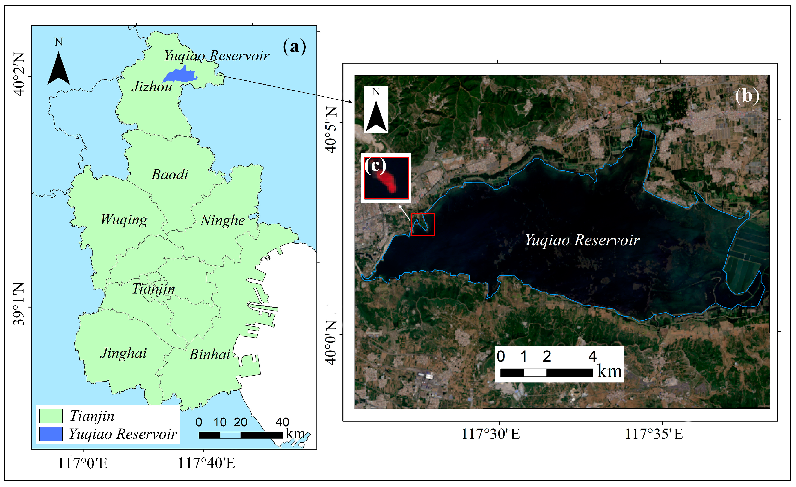
2.1. Materials

This study focuses on the eutrophic status of Yuqiao Reservoir from 1984 to 2022, whose geographical location is illustrated in Figure 1. The reservoir boundary is delineated by NDWI for clipping the study area.
The satellite images are Landsat surface reflectance data, all of which have been atmospherically corrected using the Land Surface Reflectance Code (LaSRC) and Landsat Ecosystem Disturbance Adaptive Processing System (LEDAPS) [31]. LaSRC and LEDAPS are atmospheric correction methods based on the 6S radiative transfer model specially designed for Landsat satellites. The 6S radiative transfer model considers the effect of Rayleigh scattering on radiative transfer, so this study uses Rayleigh-corrected data. LaSRC is an atmospheric correction program designed by USGS for Landsat 8 data. LEDAPS is software for automated production of Landsat 4, 5, 7 surface reflectance, which is funded by NASA [32].
The datasets included Landsat 5 data from 1984 to 2000, Landsat 7 data from 2000 to 2020, Landsat 8 data from 2014 to 2021, and Landsat 9 data from 2021 to 2022. A total of 632 high-quality valid images were visually screened to exclude images heavily affected by clouds. Specifically, the datasets consisted of 245 Landsat 5 images, 192 Landsat 7 images, 169 Landsat 8 images, and 26 Landsat 9 images. The aforementioned satellite remote sensing images were obtained from the United States Geological Survey (USGS, https://earthexplorer.usgs.gov/) (accessed on 1 July 2023). Detailed information about the basic datasets has been presented in Table 1.
To evaluate the performance of the method in this study, we acquired a one-view Gaofen-2 Panchromatic Multi-spectral (GF-2 PMS) image of the study area on 26 May 2019, from the Land Observing Satellite Data Service Platform (https://data.cresda.cn/) (accessed on 1 July 2023). The above data were ortho-corrected and atmospherically corrected based on the Flaash module of ENVI. They were fused to a product with a resolution of 1 m using panchromatic and multi-spectral bands. In addition, this study obtained water level measurements at the Yuqiao Reservoir dam monitoring site from August 2021 to November 2022, using the National Water Quality Automatic Supervision Platform (https://szzdjc.cnemc.cn/) (accessed on 1 July 2023). The collected data were utilized to perform an inversion of historical water levels.

2.2. Method Description

Despite the high applicability of many remote sensing indices such as normalized difference vegetation index (NDVI), floating algae index (FAI), and normalized difference water index (NDWI) in vegetation monitoring and water extraction, determining an appropriate threshold remains a challenge [33]. Meanwhile, ABs and AV often exhibit similar spectral properties, characterized by low reflectance in the blue–violet and red bands but increased reflectance in the near-infrared band [21]. It is difficult to detect ABs in aquatic ecosystems by traditional remote sensing classification methods. Therefore, we combined several remote sensing indexes to distinguish VS from water using DTM; thereafter, we employed VPF to extract the range of AV and thereby facilitated the identification of ABs.
Figure 2 shows the overall workflow of the AB extraction. Firstly, we calculated and counted the NDVI, NDWI, and FAI of the pixels and used DTM to distinguish VS from open water. Secondly, we selected images with normal and low water levels during the growing season and an appropriate VPF threshold to extract the annual maximum extent of AV. Finally, we took the intersection of the VS and AV range and inverted it to obtain the distribution of ABs.

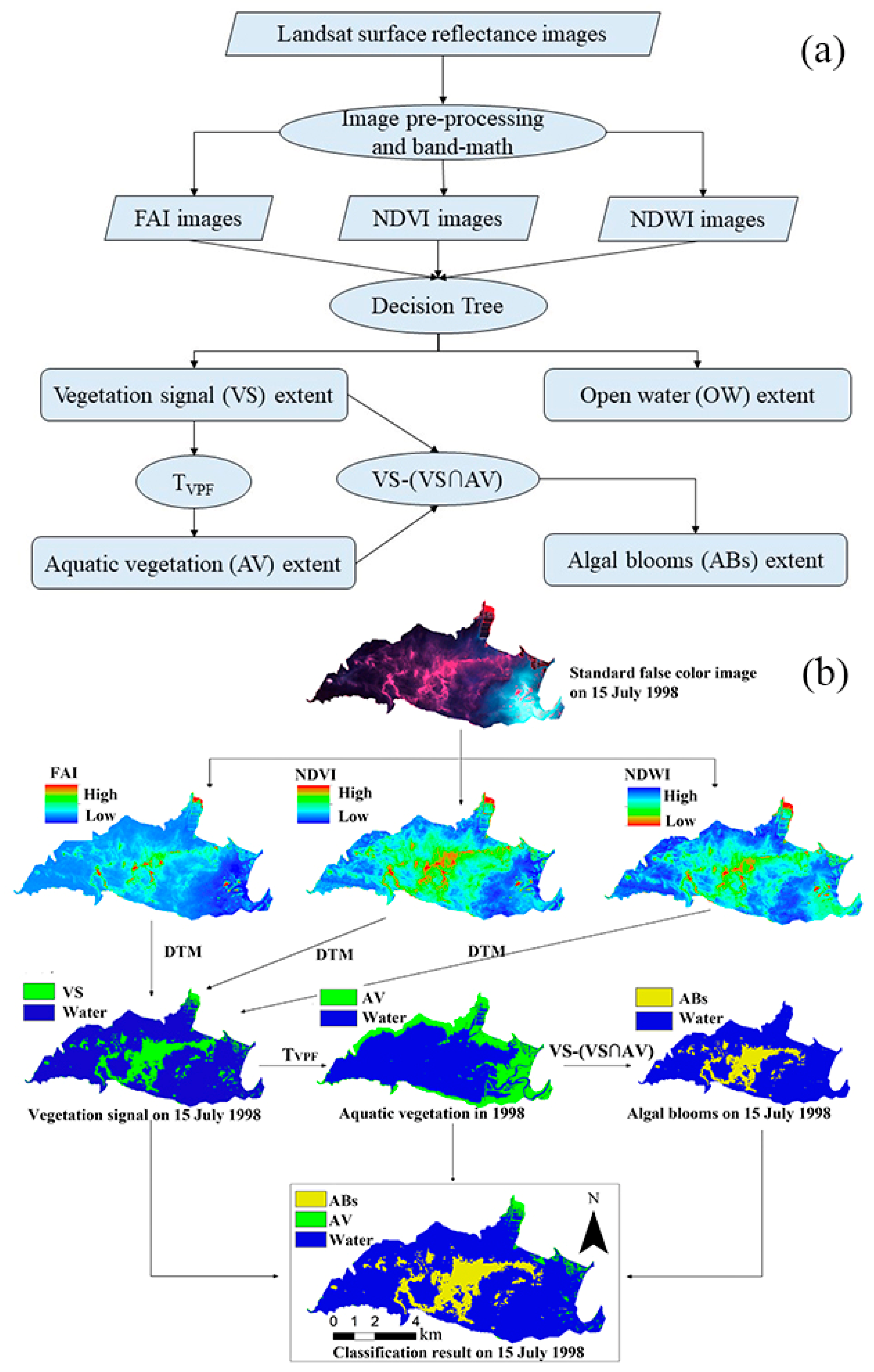
2.2.1. Multi-Index Decision Tree Model

The multi-index decision tree model is used to distinguish VS from water bodies, where VS is defined as a collection of AV and ABs. We selected 500 sample points in representative images based on visual interpretation. The selection of sample points follows the following principles: we select ABs with different intensities, AV with different growth states (limited by the spatial resolution of Landsat, AV and ABs cannot be visually distinguished, so the sample points of these two features are mixed as VS), and pure water in different seasons. The detailed information on the selected sample points is shown in Table 2. We calculated and counted the NDVI, FAI, and NDWI of the above sample points and explored the quantitative relationship of multiple indexes to determine the multi-index decision tree model that distinguishes VS and water bodies. The NDVI, FAI, and NDWI were calculated using the following equations.
NDVI = (RNIRRRED)/(RNIR + RRED)
FAI = RNIRRRED
RRED’ = RRED + (RSWIRRRED) * (λNIRλRED)/(λSWIRλRED)
NDWI = (RGREENRNIR)/(RGREEN + RNIR)
where RSWIR, RNIR, RRED, and RGREEN represent the spectral reflectance of features in the short-wave infrared, near-infrared, red, and green bands, respectively; λSWIR, λNIR, and λRED denote the central wavelengths in the short-wave infrared, near-infrared, and red bands, respectively.

2.2.2. Vegetation Presence Frequency (VPF)

The VPF represents the probability that a pixel is AV during the study period [21]. The method of separating ABs and AV using VPF relies on the following assumptions: the growth range of AV remains relatively stable for most of the year due to significant phenological characteristics [34], whereas ABs usually drift on the water surface and their growth location is dynamic [35]; and higher levels of AV generally has the effect of absorbing nitrogen and phosphorus nutrients from the water, thereby inhibiting algal growth [28]. We refer to the survey results of Yuqiao Reservoir on the plant diversity: Yuqiao Reservoir is dominated by emergent plants, mostly Phragmites australis, Schoenoplectus tabernaemontani, Typha angustifolia, and Nelumbo nucifera, which together constitute the dominant species of the emergent plant community in the lakeshore zone; only Trapa bispinosa and Nymphoides peltatum were found regarding floating-leaf plants; submerged plants include Potamogeton crispus, Potamogeton wrightii, Potamogeton crispus, Myriophyllum verticillatum, and Cera tophyllum demersum [36]. Generally speaking, the plant diversity of Yuqiao Reservoir is low, and emergent plants are dominant. Therefore, combined with the current status of specific plant types in Yuqiao Reservoir, we can ignore the interference of some rootless aquatic vegetation in this study. Furthermore, it can be hypothesized that the growth locations of AV and ABs do not overlap and the presence frequency of AV is greater than that of ABs based on the above assumptions. The VPF is calculated as follows:
V P F j = i = 1 n L v ( j , i ) n
where VPF(j) denotes the vegetation presence frequency of pixel j in n images, and Lv (j, i) represents the specific feature information extracted as shown in Section 2.2.1. A value of 1 is assigned when pixel j of image i is determined as VS, otherwise it is assigned a value of 0. n is the total number of images in the calculated time range.
After the VS and AV are successfully extracted, we utilize the AV boundary to partition the VS, with the intersection between the two regions regarded as the AV area. Conversely, the space beyond the confines of the AV boundary is classified as AB.

2.3. Accuracy Assessment

In this study, we selected GF-2 PMS to verify Landsat 8 because the high spatial resolution image has more pixels and can capture more details. The algal blooms in Yuqiao Reservoir have a mostly spotted distribution, so the range of occurrence is small. Whether the small area of algal blooms can be accurately captured in the image is our primary consideration. Therefore, we emphasize the significance of high spatial resolution for algal bloom extraction. However, GF-2 and Landsat satellites have different revisit periods, so it is difficult to find images from the same date of these satellites. Through a large number of image data retrieved, we found that on 26 May 2019, GF-2 and Landsat 8 satellites passed across the Yuqiao Reservoir, and the data quality was good and suitable for research.
Considering that the GF-2 image has only visible and near-infrared bands, only NDVI and NDWI can be used when extracting VS. According to the results of Section 2.2.1, we determined the pixel of NDVI > NDWI as VS. After masking VS using the extracted AV extent from 2019, we were able to obtain AB distribution based on GF-2 data.
The spatial resolution of Landsat 8 is lower than that of GF-2, so the area of algal blooms extracted based on Landsat 8 is generally larger than that of GF-2. When evaluating the method of extracting algal blooms, we only considered the spatial distribution trend of the extraction results based on different data sources, regardless of the specific area of algal blooms. The interclass correlation coefficient (ICC), which is a measure of the degree of agreement among multiple observations of the same subject, is defined as the ratio of the between-group variance to the total variance [37,38,39]. In this study, ICC was employed to assess the agreement between the spatial distribution patterns of ABs derived from GF-2 and Landsat sources. The closer the ICC is to 1, the closer the multiple observations are to each other and the more reliable the observations are; the closer the ICC is to 0, the greater the difference between the multiple observations is and the less reliable the observations are; if ICC is negative, the measurement process itself has a systematic bias [40]. The generally accepted ICC evaluation criteria are as follows: when the value is less than 0.4, the observation is less reliable; when it is between 0.4 and 0.59, the consistency is average; when it is between 0.6 and 0.74, the consistency is good; when the value is greater than 0.75, the consistency is trustworthy [41].

2.4. Statistical Analyses

The method was applied to the long-term Landsat images of Yuqiao Reservoir from 1984 to 2022 to investigate the spatial distribution characteristics and temporal variations of ABs. Firstly, the FAI characterizes the intensity of ABs in a single pixel [42], which can be used to describe the spatial distribution characteristics of ABs. Secondly, the floating algae coverage index (FACI) is the product of the area of ABs in a single image and the mean value of FAI, which is a comprehensive reflection of AB range and intensity [43] and can be used to describe the interannual variation trend of ABs. Finally, considering that no AB event is detected in some years and that the effectiveness of water environmental protection efforts is mostly phased [44], the occurrence of ABs in reservoirs is studied statistically in phases, taking five years as a period. The images of the ABs detected in a year are summed and superimposed each year to reflect the frequency and severity of ABs.
FACI = FAImean * AreaABs

3. Results

3.1. Method Development

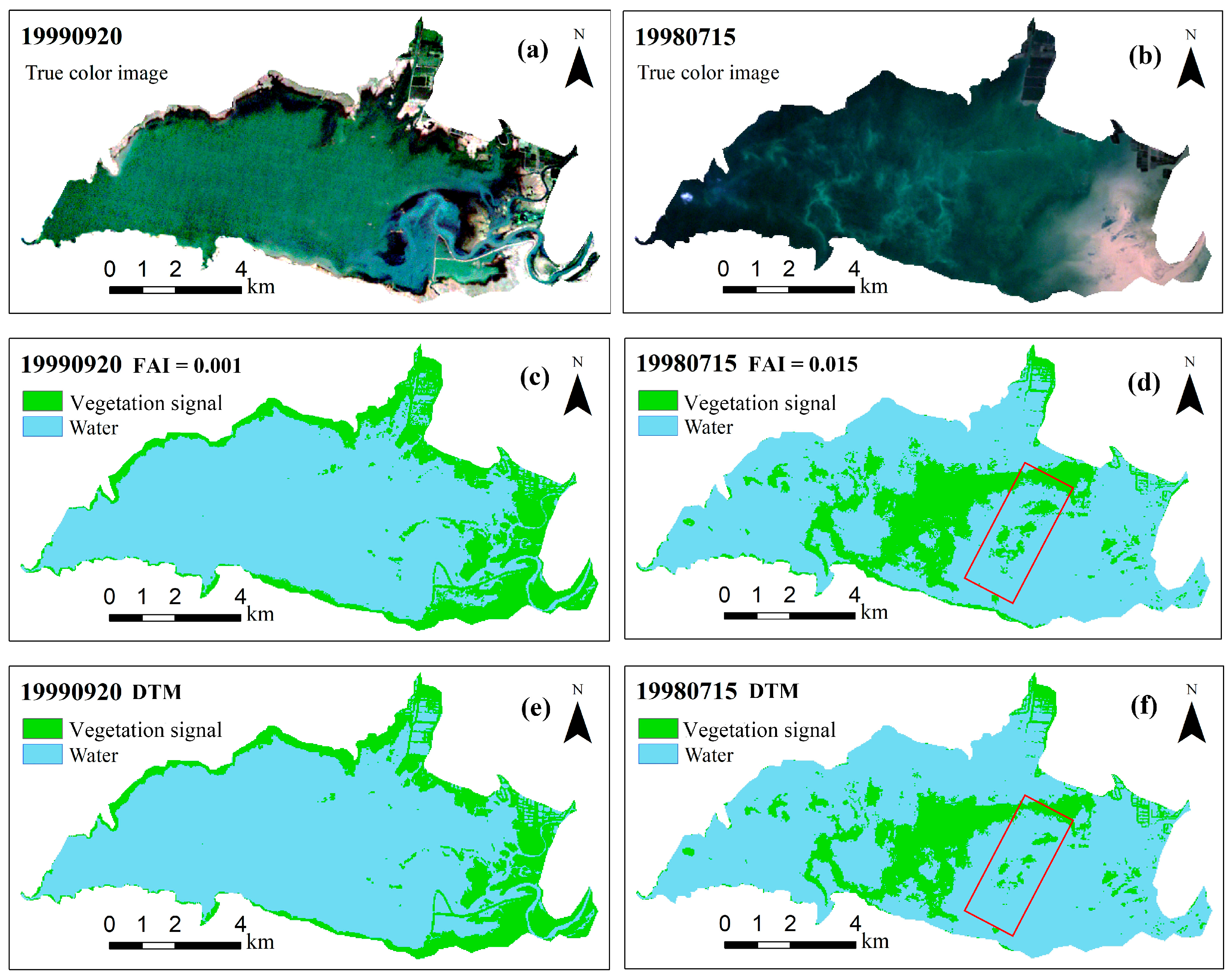
3.1.1. Separating VS and Water

Analysis of the multi-index box plot (Figure 3a) reveals that water bodies generally exhibit an NDVI and FAI below 0, whereas their NDWI is typically above 0. In contrast, VS generally displays an NDVI and FAI above 0, while the NDWI tends to be below 0. However, it should be noted that the results cannot exclude the case that water may exhibit an FAI and NDVI above 0, or that VS may express an NDWI above 0. Therefore, it is not reliable to solely rely on a certain index or a few indexes to distinguish all features. By comparing the range of three indexes in Figure 3a, it has been observed that the NDWI generally surpasses NDVI and FAI for water, whereas the NDWI tends to be lower than NDVI and FAI values for VS. This method can effectively get rid of the interference of threshold selection and improve the accuracy of VS extraction. A multi-index decision tree model has been developed as follows:
V e g e t a t i o n   s i g n a l = 1 ,   F A I     N D W I   &   N D V I     N D W I 0 ,   O t h e r
where 1 indicates that the feature is VS, and 0 indicates that the feature is other, which indicates water in this study.
FAI has a good effect on VS extraction in eutrophic water. Therefore, we compared the results of VS extraction based on FAI and the multi-index decision tree model. As shown in Figure 4, the multi-index decision tree model uses the same extraction equation (Equation (7)) for water bodies with differing turbidity, so the calculation amount is small. However, the FAI threshold of 0.001 has better classification results when the water is clear (Figure 4c); while the FAI threshold of 0.015 is more suitable for classification when the water is turbid (Figure 4d). Furthermore, Figure 4b displays that a large amount of sediment flow from the eastern part of the reservoir. Compared with the VS extracted by multi-index DTM, there are many misclassifications in the eastern part of the reservoir when only FAI is used, as shown in the red box of Figure 4d,f.

3.1.2. Separating ABs and AV

The calculation of VPF mainly involves two issues including image selection and threshold determination:
  • Image selection
One of the tasks of this study is to delineate the maximum annual growth range of AV, and two main factors are considered in image selection: the growth condition of the AV and the effects of flooding due to high water levels.
The growth condition of AV was taken into consideration to select the appropriate period for AV extraction [45]. Based on the Standard for Fishery Resources Survey of Chinese Reservoirs, Yuqiao Reservoir is classified as a warm temperate subhumid continental monsoon climate with four distinct seasons [46]. Specifically, the freezing period with minimal vegetation occurs from December to February of the following year, while the initial stage of plant growth typically spans from March to April. The peak growth period for most AV species typically extends from May to October, with degradation of AV commencing from November onwards [47]. Therefore, the period from May to October is selected for extracting AV in this study due to its maximal growth and stability during this period.
Additionally, Yuqiao Reservoir, as a human-made lake, is highly influenced by frequent water storage and discharge [48]. When the reservoir is impounded, the water level rises and much AV is submerged, resulting in inaccurate extraction of the AV range; moreover, AV extraction is more likely to be affected due to the small number of Landsat images. Therefore, the accuracy of AV extraction can be improved by using the measured water level data to invert the historical water level and then removing the high water level images. The mudflat located in the northwest of Yuqiao Reservoir (Figure 1c) exists year-round with higher AV growing on it, and the overall water quality is good with few ABs occurring around it [47,48,49]. The historical water level can be inverted by establishing the relationship between the flooding area and the water level in this area (Figure 3b).
Based on the measured water level data from the national monitoring station, the following mathematical relationship is developed. Statistically, 18.3–18.6 m is the best range for removing the high water level images. Combined with visual interpretation, the images above the water level threshold can be eliminated, which contributes to the selection of the VPF threshold and the extraction of AV.
Y = 7.9740X + 8.5254
where Y is the water level (m) on the dam of Yuqiao Reservoir, and X is the flooding area (km2) in Figure 1c.
We compared the differences in the interannual maximum range of aquatic vegetation before and after the removal of high water level images, as shown in Figure 5. Figure 5a is the maximum interannual growth range of AV extracted before removing high water level images in 2002; Figure 5b is the AV result after removing high water level images in 2002. If the images of high water level are not excluded, it may lead to a reduction in the maximum growth range of AV and subsequently affect the further extraction of ABs.
  • VPF threshold determination
The VPF ranges from 0 to 1. Considering the fixed location of AV, the VPF should be greater than or equal to 0.5 [21]. Images of Taihu Lake in a year were subdivided according to the growth state of AV based on MODIS data to determine multiple VPF thresholds for different growth periods [24], among which the VPF threshold in the flourishing period (June to October) was 0.85; VPF thresholds suitable for different lakes were explored based on Sentinel-2 [21], among which 0.5 was used as the VPF threshold in Hongze Lake and Hulun Lake because of low AB frequency. Yuqiao Reservoir plays a crucial role as part of the Luanhe-Tianjin Water Diversion Project [50]. Although water quality has declined in recent years [51], the incidence of ABs remains relatively low. Given that this study employs Landsat images with a long acquisition period and a limited number of images, a VPF threshold of 0.5 has been selected based on previous research.

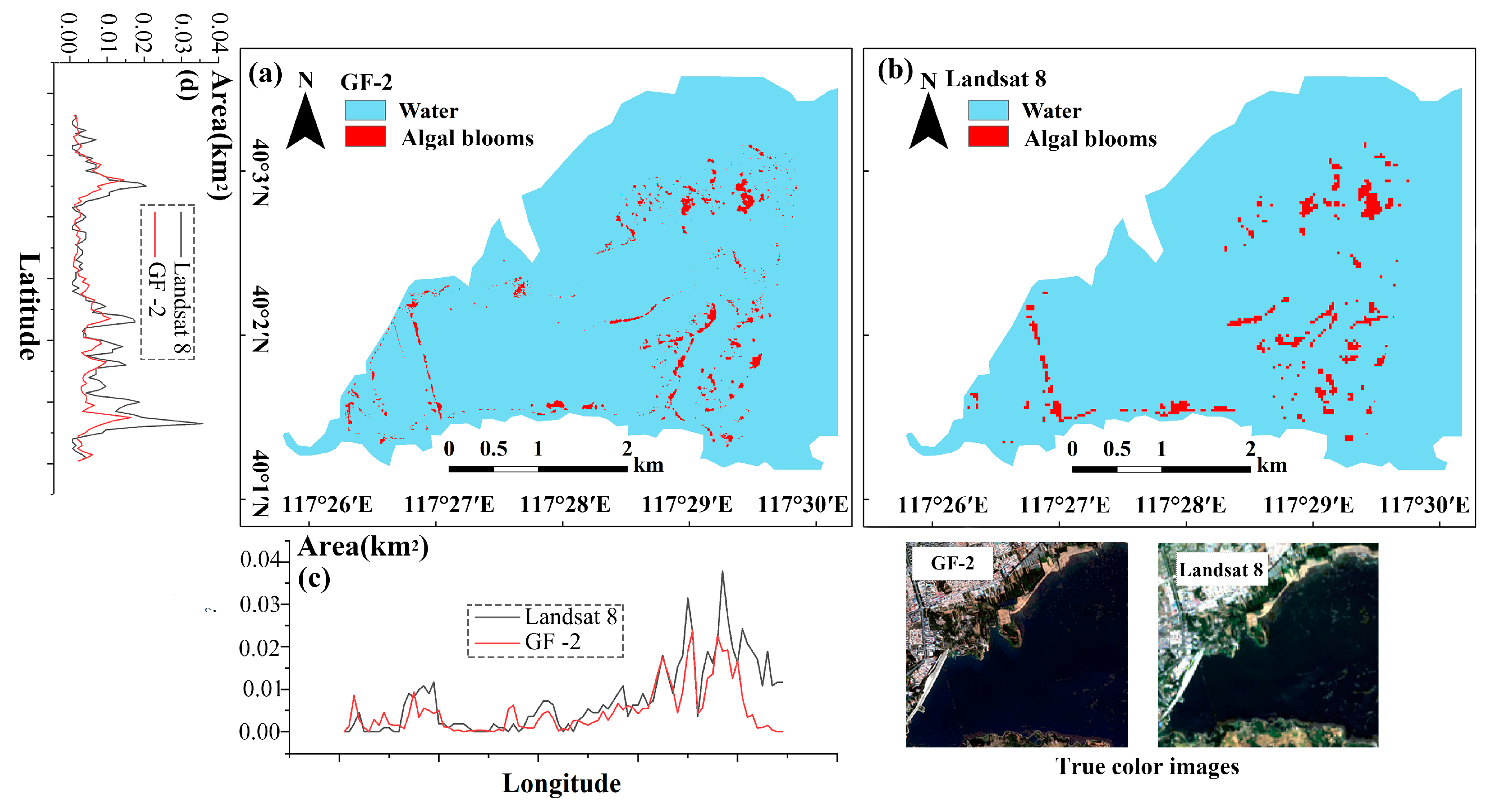
3.2. Validation by GF-2 PMS Data

We compared the AB area of GF-2 and Landsat 8 images acquired on the same date (26 May 2019) to assess the spatial consistency of AB distribution trends. Figure 6 presents the statistical analysis of the changes in ABs along both longitudinal and latitudinal directions: the ICC of AB area derived from Landsat 8 and GF-2 images was found to be 0.822 in the longitude direction, 0.771 in the latitude direction, and 0.797 overall. The spatial distribution trends of AB area based on Landsat and GF-2 showed high consistency, indicating that the applied method had high accuracy for AB extraction.

3.3. Spatial and Temporal Dynamics of AB Distribution

We mapped the distribution of algal blooms in Yuqiao Reservoir periodically, shown in Figure 7, and calculated the variation trends of ABs in longitude and latitude in different periods, shown in Figure 8. Spatially, the water affected by ABs was widespread within the reservoir, spanning from 117°28′00″E to 117°35′00″E and 40°01′00″N to 40°04′00″N. The distribution of water affected by ABs was also non-uniform, with a primary concentration occurring from 117°29′00″E to 117°34′30″E and 40°02′40″N to 40°03′36″N. Furthermore, the intensity of ABs in the north of the reservoir was higher than that in other areas. In terms of temporal analysis, a total of 72 AB events were detected from 632 Landsat images screened in this study, covering the period from 1984 to 2022. The frequency of ABs observed during the study periods reached up to 11.40%, suggesting that water eutrophication in Yuqiao Reservoir was severe. Although there were differences in AB intensity during different periods, an overall increasing-then-decreasing trend in AB intensity was observed from 1984 to 2022. The composite FACI increased from 2.81 from 1984–1988 to 427.35 from 2004–2008 and then decreased to 99.37 from 2019–2022. The variation of AB intensity in longitude was significantly higher than that in latitude. The severe period of ABs was mainly concentrated from 1994–1998, 1999–2003, and 2004–2008 in longitude but only concentrated from 2004–2008 in latitude. In contrast, the variation of AB intensity in other research periods was weak in longitude and latitude.
From Figure 7 and Figure 8, we also found that: FACI is almost close to 0 from 1984–1993 and 2009–2013. We considered the following reasons: Yuqiao Reservoir officially supplied water to Tianjin citizens in 1983, and the water pollution in the following years was relatively weak; the study from 2009–2013 is mainly based on Landsat 7 data. However, after 2003, the Landsat 7 image band was missing, resulting in incomplete images. Therefore, when Landsat 7 images were used for algal bloom extraction, algal blooms were underestimated.

4. Discussions

4.1. Advantages of the Method

Eutrophication in reservoirs threatens water quality safety and human health, the most typical manifestation of which is ABs [52]. We established an improved AB extraction method and successfully applied this approach to the historical images of Yuqiao Reservoir. This method provides an attempt to identify ABs in shallow lakes and has the potential to be extended to other eutrophic water. The advantages of the method are mainly reflected in three aspects:
Firstly, this study selects Landsat long-term series remote sensing images. MODIS images are not conducive to the study of small lakes such as reservoirs due to their low spatial resolution, despite the abundance of data available [53]; despite Sentinel data’s advantages in spatial and temporal resolution [54], its satellite launch time can only be traced back to 2015, making it less suitable for long-term research. While GF-2 data boast a submeter spatial resolution and a mere 5-day revisit period, its restricted access and earliest imaging time fail to comply with the study’s requirements. In contrast, the Landsat series images, which have been successfully used since 1984, provide high spatial resolution and demonstrate unrestricted image acquisition, thus proving advantageous for long-term studies. Relevant satellite parameters can be found in Table 3.
Secondly, this study combines multiple remote sensing indexes to extract VS. It is difficult to distinguish the mixed pixels of water and VS only based on FAI because FAI is weak in identifying low-density cyanobacteria, and it is easy to misclassify highly turbid water as VS. However, the combination of multiple indexes and DTM can improve the accuracy of object extraction. Additionally, different FAI thresholds are selected for images from different periods and locations. The threshold selection creates not only a large workload but is also prone to misclassification. However, the method in this study gets rid of the threshold selection and greatly reduces the amount of computation.
Finally, we introduce the water level to facilitate the determination of the VPF threshold. The annual maximum growth range of AV is extracted to obtain a more accurate location of ABs in this study.

4.2. Limitations of the Method

The method of this study is also limited by some factors. There are fewer available images for the extracting of AV extent due to the long revisit period of the Landsat satellite and the poor quality of some images. And the number of images available in some years is small. We use image interpolation technology to supplement the data with images of the same season in adjacent years based on the similarity of plant phenology in the same seasons to realize the continuous monitoring of algal blooms. In addition, the number of available images directly affects the selection of the VPF threshold, which further influences the extraction of the growth range of AV. Moreover, we select 0.5 as the VPF threshold based on the empirical conclusions of other scholars in this study, but the AV of some images is misjudged as ABs which are mostly distributed at the land–water boundary. To address this issue, we propose filtering out misclassified pixels by establishing a buffer zone for the AV boundary (Figure 9). Finally, the selection of VS and water sample points in this study is based on the visual interpretation of the images, which is more subjective. However, standard false-color images typically display VS as red and water as black or blue–black, resulting in a significant color contrast between VS and water. As a result, the probability of error in selecting sample points is relatively small.
In summary, the quantity and quality of images are the main constraints of this study, and we expect to compensate for the shortcomings of this study with higher resolution and shorter periods of remote sensing images.

4.3. Human Factors Influencing the Spatial and Temporal Variations of ABs

The spatial and temporal patterns of AB intensity in Yuqiao Reservoir indicate that the ABs have gradually spread throughout the reservoir, leading to a continuous deterioration of the aquatic ecosystem. Although some progress has been made in recent years, the current water quality in the reservoir still poses significant safety hazards when compared to the initial stages of the water supply.
Human activities affect algal outbreaks in Yuqiao Reservoir mainly through various types of pollution [55]. On the one hand, the Panjiakou Reservoir upstream of Yuqiao Reservoir has been vigorously developing fish cage culture [30]; it was initially restricted to the inlet of the upper Panjiakou Reservoir in the late 1980s. The scale of fish farming was expanded in the early 1990s. By 2007, net fishing had spread throughout the majority of the reservoir, accounting for approximately 1.7% of the total reservoir area and featuring around 17,000 boxes [56]. In 2016, the local government implemented measures to clean the cages, with cleaning work completed by 2017, resulting in the restoration of water quality downstream and throughout the reservoir. Correspondingly, AB intensity in Yuqiao Reservoir increased from 2.81 (1984–1988) to 427.35 (2004–2008), and the water quality improved from 2014–2018, however, it still could not be restored to the state before being polluted. On the other hand, industrial and agricultural pollution in the Yuqiao watershed affects water quality safety. Industrial pollution is mainly distributed in Zunhua City and Jizhou District. According to the 2004 survey statistics [57], Zunhua City had 207 sewage enterprises, and the annual discharge of industrial sewage was 18.57 million t. Zunhua City occupied 58% of the Yuqiao watershed area, and various types of land that can contribute to non-point source pollution amounted to about 1317 km2 in Zunhua where the amount of pesticide and fertilizer application was 26,808 t [58]. There are two main pathways of pesticides and fertilizers: absorption by crops or retention in the soil with the subsequent flow into nearby water sources during rainfall-runoff events which threatens water quality [59].
The pollution of Yuqiao Reservoir predominantly results from the input of various nutrients from upstream and surrounding regions. Tianjin Yuqiao Reservoir Management Center carried out a water purification project [60] to protect the ecological environment and promote comprehensive, coordinated, and sustainable socio-economic development. Firstly, a pre-reservoir project was implemented. The pre-reservoir project involved planting emergent plants, submerged plants, and phytoplankton by the law to effectively absorb and decompose water pollutants for water purification. The relevant departments established the pre-reservoir project at the Guo River upstream of the Yuqiao Reservoir. The pre-reservoir project could effectively purify the sewage from upstream and was put into trial operation in August 2017. Secondly, the phased closing of reservoirs and fishing bans was carried out. This work is one of the important measures to relieve the pressure on water ecology and protect fishery resources. The Jizhou District Government has been carrying out this policy since 2017, with specific closure periods including 16 April–15 July 2017, 16 December 2021–28 February 2022, etc. In addition, there are other projects such as the management of the reservoir channel, the transformation of the sewage pipe network in the nearby villages, the water ecological restoration, and the ecological protection of the lakeshore, which play an important role in the protection of water quality.

5. Conclusions

In conclusion, we have presented a method for effectively distinguishing algal blooms (ABs) from water and aquatic vegetation (AV) in shallow lakes using satellite data. The method, comprising three main steps, addresses the challenge of differentiating ABs from AV and offers a reliable solution for AB identification in aquatic ecosystems. By integrating multiple remote sensing indexes, we successfully extract the vegetation signal (VS) and determine the AV range based on vegetation presence frequency (VPF) and normal/low water level images. The intersection of the VS and AV range enables us to accurately locate ABs. The validation results, with an interclass correlation coefficient (ICC) of 0.822 and 0.771 in the longitude and latitude directions, respectively, and an overall ICC of 0.797, demonstrate the method’s effectiveness in capturing the spatial distribution trend of ABs using both Landsat and GF-2 satellites.
Applying our method to Yuqiao Reservoir, we visualize the geographical distribution of ABs from 1984 to 2022, revealing their wide distribution and concentration in the northern region. Over the past 39 years, ABs have shown an initial increase followed by a subsequent decrease. However, despite improvements in water quality, challenges persist, as AB outbreaks are primarily attributed to human activities such as fish cage culture and pollution from surrounding industries and agriculture. To alleviate the pressure on water ecosystems, robust water purification projects are crucial.
Our improved method, designed for Landsat images with long revisit periods, showcases its potential in AB identification. With further optimization and validation, it holds promise for application with various satellite sensors, enabling more effective spatial–temporal monitoring of vegetation signals in inland lakes. This advancement will contribute to a better understanding of critical ecological issues, particularly water eutrophication.

Author Contributions

Conceptualization, H.D. and Y.L.; methodology, H.D., X.H., W.C. and D.L.; software, D.L. and X.H.; supervision, H.D. and X.H.; project administration, X.H.; funding acquisition, H.D., Y.L., X.H. and D.L. All authors have read and agreed to the published version of the manuscript.

Funding

This research was funded by Ministry of Science and Technology of the People’s Republic of China (grant number 2021FY101000 and 2022YFF1301002); Science and Technology Bureau of Tianjin (Grant Number: 22ZYJDJC00140); Open Research Fund Program of LIESMARS (Grant Number: 21R01); and the Graduate Student Research Innovation Program of Tianjin (Grant Number: 2022SKY076).

Data Availability Statement

Publicly available datasets were analyzed in this study. These data can be found here: https://earthexplorer.usgs.gov/; https://data.cresda.cn/; https://szzdjc.cnemc.cn/. (accessed on 1 July 2023).

Conflicts of Interest

The authors declare no conflict of interest.

References

  1. Pekel, J.-F.; Cottam, A.; Gorelick, N.; Belward, A.S. High-resolution mapping of global surface water and its long-term changes. Nature 2016, 540, 418–422. [Google Scholar] [CrossRef]
  2. Huang, S.; Zhang, K.; Lin, Q.; Liu, J.; Shen, J. Abrupt ecological shifts of lakes during the Anthropocene. Earth-Sci. Rev. 2022, 227, 103981. [Google Scholar] [CrossRef]
  3. Fang, C.; Song, K.; Paerl, H.W.; Jacinthe, P.A.; Wen, Z.; Liu, G.; Tao, H.; Xu, X.; Kutser, T.; Wang, Z. Global divergent trends of algal blooms detected by satellite during 1982–2018. Glob. Chang. Biol. 2022, 28, 2327–2340. [Google Scholar] [CrossRef]
  4. Dalby, S. Climate change: New dimensions environmental security. RUSI J. 2013, 158, 34–43. [Google Scholar] [CrossRef]
  5. Alexander, T.J.; Vonlanthen, P.; Seehausen, O. Does eutrophication-driven evolution change aquatic ecosystems? Philos. Trans. R. Soc. B Biol. Sci. 2017, 372, 20160041. [Google Scholar] [CrossRef]
  6. Codd, G.A. Cyanobacterial toxins, the perception of water quality, and the prioritisation of eutrophication control. Ecol. Eng. 2000, 16, 51–60. [Google Scholar] [CrossRef]
  7. Qin, B.; Yang, G.; Ma, J.; Wu, T.; Li, W.; Liu, L.; Deng, J.; Zhou, J. Spatiotemporal changes of cyanobacterial bloom in large shallow eutrophic Lake Taihu, China. Front. Microbiol. 2018, 9, 451. [Google Scholar] [CrossRef]
  8. Zhu, S.; Wu, Y.; Ma, X. Deep Learning-Based Algal Bloom Identification Method from Remote Sensing Images—Take China’s Chaohu Lake as an Example. Sustainability 2023, 15, 4545. [Google Scholar] [CrossRef]
  9. Jing, Y.; Zhang, Y.; Hu, M.; Chu, Q.; Ma, R. MODIS-satellite-based analysis of long-term temporal-spatial dynamics and drivers of algal blooms in a plateau lake Dianchi, China. Remote Sens. 2019, 11, 2582. [Google Scholar] [CrossRef]
  10. Lunetta, R.S.; Schaeffer, B.A.; Stumpf, R.P.; Keith, D.; Jacobs, S.A.; Murphy, M.S. Evaluation of cyanobacteria cell count detection derived from MERIS imagery across the eastern USA. Remote Sens. Environ. 2015, 157, 24–34. [Google Scholar] [CrossRef]
  11. Mishra, S.; Mishra, D. A novel remote sensing algorithm to quantify phycocyanin in cyanobacterial algal blooms. Environ. Res. Lett. 2014, 9, 114003. [Google Scholar] [CrossRef]
  12. Ogashawara, I.; Mishra, D.R.; Gitelson, A.A. Remote sensing of inland waters: Background and current state-of-the-art. In Bio-Optical Modeling and Remote Sensing of Inland Waters; Elsevier: Amsterdam, The Netherlands, 2017; pp. 1–24. [Google Scholar]
  13. Meinson, P.; Idrizaj, A.; Nõges, P.; Nõges, T.; Laas, A. Continuous and high-frequency measurements in limnology: History, applications, and future challenges. Environ. Rev. 2016, 24, 52–62. [Google Scholar] [CrossRef]
  14. Pan, D.; Ma, R. Several key problems of lake water quality remote sensing. J. Lake Sci. 2008, 20, 139–144. [Google Scholar]
  15. Gai, Y.; Yu, D.; Zhou, Y.; Yang, L.; Chen, C.; Chen, J. An improved model for chlorophyll-a concentration retrieval in coastal waters based on UAV-Borne hyperspectral imagery: A case study in Qingdao, China. Water 2020, 12, 2769. [Google Scholar] [CrossRef]
  16. Hu, C.; Muller-Karger, F.E.; Taylor, C.J.; Carder, K.L.; Kelble, C.; Johns, E.; Heil, C.A. Red tide detection and tracing using MODIS fluorescence data: A regional example in SW Florida coastal waters. Remote Sens. Environ. 2005, 97, 311–321. [Google Scholar] [CrossRef]
  17. Hou, T.; Sun, W.; Chen, C.; Yang, G.; Meng, X.; Peng, J. Marine floating raft aquaculture extraction of hyperspectral remote sensing images based decision tree algorithm. Int. J. Appl. Earth Obs. Geoinf. 2022, 111, 102846. [Google Scholar] [CrossRef]
  18. Hu, C. A novel ocean color index to detect floating algae in the global oceans. Remote Sens. Environ. 2009, 113, 2118–2129. [Google Scholar] [CrossRef]
  19. Hu, C.; Lee, Z.; Ma, R.; Yu, K.; Li, D.; Shang, S. Moderate resolution imaging spectroradiometer (MODIS) observations of cyanobacteria blooms in Taihu Lake, China. J. Geophys. Res. Ocean. 2010, 115. [Google Scholar] [CrossRef]
  20. Shurin, J.B.; Abbott, R.L.; Deal, M.S.; Kwan, G.T.; Litchman, E.; McBride, R.C.; Mandal, S.; Smith, V.H. Industrial-strength ecology: Trade-offs and opportunities in algal biofuel production. Ecol. Lett. 2013, 16, 1393–1404. [Google Scholar] [CrossRef]
  21. Pu, J.; Song, K.; Liu, G.; Wen, Z.; Fang, C.; Hou, J.; Lv, Y. Differentiation of Algal Blooms and Aquatic Vegetation in Chinese Lakes Using Modified Vegetation Presence Frequency Index Method. Chin. Geogr. Sci. 2022, 32, 792–807. [Google Scholar] [CrossRef]
  22. Luo, J.; Ma, R.; Duan, H.; Hu, W.; Zhu, J.; Huang, W.; Lin, C. A new method for modifying thresholds in the classification of tree models for mapping aquatic vegetation in Taihu Lake with satellite images. Remote Sens. 2014, 6, 7442–7462. [Google Scholar] [CrossRef]
  23. Qing, S.; Runa, A.; Shun, B.; Zhao, W.; Bao, Y.; Hao, Y. Distinguishing and mapping of aquatic vegetations and yellow algae bloom with Landsat satellite data in a complex shallow Lake, China during 1986–2018. Ecol. Indic. 2020, 112, 106073. [Google Scholar] [CrossRef]
  24. Liu, X.; Zhang, Y.; Shi, K.; Zhou, Y.; Tang, X.; Zhu, G.; Qin, B. Mapping aquatic vegetation in a large, shallow eutrophic lake: A frequency-based approach using multiple years of MODIS data. Remote Sens. 2015, 7, 10295–10320. [Google Scholar] [CrossRef]
  25. Fang, C.; Luo, K.; Kong, Y.; Lin, H.; Ren, Y. Evaluating performance and elucidating the mechanisms of collaborative development within the Beijing–Tianjin–Hebei region, China. Sustainability 2018, 10, 471. [Google Scholar] [CrossRef]
  26. Yue, A.; Zeng, Q.; Wang, H. Remote sensing long-term monitoring of cyanobacterial blooms in yuqiao reservoir. Remote Sens. Technol. Appl. 2020, 35, 694–701. [Google Scholar]
  27. Cao, X.; Wang, C.; Lu, Y.; Zhang, M.; Khan, K.; Song, S.; Wang, P.; Wang, C. Occurrence, sources and health risk of polyfluoroalkyl substances (PFASs) in soil, water and sediment from a drinking water source area. Ecotoxicol. Environ. Saf. 2019, 174, 208–217. [Google Scholar] [CrossRef]
  28. Zhang, C.; Gao, X.; Wang, L.; Chen, X. Modelling the role of epiphyton and water level for submerged macrophyte development with a modified submerged aquatic vegetation model in a shallow reservoir in China. Ecol. Eng. 2015, 81, 123–132. [Google Scholar] [CrossRef]
  29. Zhang, Y.; Jeppesen, E.; Liu, X.; Qin, B.; Shi, K.; Zhou, Y.; Thomaz, S.M.; Deng, J. Global loss of aquatic vegetation in lakes. Earth-Sci. Rev. 2017, 173, 259–265. [Google Scholar] [CrossRef]
  30. Yang, F.; Sun, C.; Wang, H.; Hu, X.; Wang, S.; Zhang, M.; Zhang, L.; Zhong, J. Significant spatiotemporal variability of nitrous oxide emissions from a temperate reservoir experiencing intensive aquaculture disturbance. Agric. Ecosyst. Environ. 2023, 348, 108427. [Google Scholar] [CrossRef]
  31. Song, C.; Woodcock, C.E.; Seto, K.C.; Lenney, M.P.; Macomber, S.A. Classification and change detection using Landsat TM data: When and how to correct atmospheric effects? Remote Sens. Environ. 2001, 75, 230–244. [Google Scholar] [CrossRef]
  32. Cao, X.; Jiang, H.; Zhang, Z.; He, G.; Wang, M.; Long, T.; Wang, G.; Zhang, X. Research progress of Landsat series satellite surface reflectivity products. Surv. Mapp. Spat. Geogr. Inf. 2019, 42, 4. [Google Scholar]
  33. Bijeesh, T.V.; Narasimhamurthy, K.N. Surface water detection and delineation using remote sensing images: A review of methods and algorithms. Sustain. Water Resour. Manag. 2020, 6, 68. [Google Scholar] [CrossRef]
  34. Wersal, R.M.; Madsen, J.D. Designing and using phenological studies to define management strategies for aquatic plants. J. Aquat. Plant Manag. 2018, 56, 83–89. [Google Scholar]
  35. Ardyna, M.; Mundy, C.; Mayot, N.; Matthes, L.C.; Oziel, L.; Horvat, C.; Leu, E.; Assmy, P.; Hill, V.; Matrai, P.A. Under-ice phytoplankton blooms: Shedding light on the “invisible” part of Arctic primary production. Front. Mar. Sci. 2020, 7, 608032. [Google Scholar] [CrossRef]
  36. Investigation and analysis on biodiversity of large aquatic plants in Yuqiao Reservoir. Mod. Agric. Sci. Technol. 2018, 3.
  37. Bland, J.; Altman, D. A note on the use of the intraclass correlation coefficient in the evaluation of agreement between two methods of measurement. Comput. Biol. Med. 1990, 20, 337–340. [Google Scholar] [CrossRef]
  38. Nakagawa, S.; Johnson, P.C.; Schielzeth, H. The coefficient of determination R 2 and intra-class correlation coefficient from generalized linear mixed-effects models revisited and expanded. J. R. Soc. Interface 2017, 14, 20170213. [Google Scholar] [CrossRef]
  39. Yen, M.; Lo, L.-H. Examining test-retest reliability: An intra-class correlation approach. Nurs. Res. 2002, 51, 59–62. [Google Scholar] [CrossRef]
  40. Chen, C.-C.; Barnhart, H.X. Comparison of ICC and CCC for assessing agreement for data without and with replications. Comput. Stat. Data Anal. 2008, 53, 554–564. [Google Scholar] [CrossRef]
  41. Cicchetti, D.V. Guidelines, criteria, and rules of thumb for evaluating normed and standardized assessment instruments in psychology. Psychol. Assess. 1994, 6, 284. [Google Scholar] [CrossRef]
  42. Zhang, Y.; Ma, R.; Duan, H.; Loiselle, S.A.; Xu, J.; Ma, M. A novel algorithm to estimate algal bloom coverage to subpixel resolution in Lake Taihu. IEEE J. Sel. Top. Appl. Earth Obs. Remote Sens. 2014, 7, 3060–3068. [Google Scholar] [CrossRef]
  43. Wang, Q.; Sun, L.; Zhu, Y.; Wang, S.; Duan, C.; Yang, C.; Zhang, Y.; Liu, D.; Zhao, L.; Tang, J. Hysteresis effects of meteorological variation-induced algal blooms: A case study based on satellite-observed data from Dianchi Lake, China (1988–2020). Sci. Total Environ. 2022, 812, 152558. [Google Scholar] [CrossRef]
  44. Lehman, P.K.; Geller, E.S. Behavior analysis and environmental protection: Accomplishments and potential for more. Behav. Soc. Issues 2004, 13, 13–33. [Google Scholar] [CrossRef]
  45. Chen, C.; He, B.; Guo, L.; Zhang, Y.; Xie, X.; Chen, Z. Identifying critical climate periods for vegetation growth in the Northern Hemisphere. J. Geophys. Res. Biogeosci. 2018, 123, 2541–2552. [Google Scholar] [CrossRef]
  46. Zhang, T.; Yang, Y.; Ni, J.; Xie, D. Construction of an integrated technology system for control agricultural non-point source pollution in the Three Gorges Reservoir Areas. Agric. Ecosyst. Environ. 2020, 295, 106919. [Google Scholar] [CrossRef]
  47. Li, T.; Chu, C.; Zhang, Y.; Ju, M.; Wang, Y. Contrasting eutrophication risks and countermeasures in different water bodies: Assessments to support targeted watershed management. Int. J. Environ. Res. Public Health 2017, 14, 695. [Google Scholar] [CrossRef]
  48. Xu, Y.; Xie, R.; Wang, Y.; Sha, J. Spatio-temporal variations of water quality in Yuqiao Reservoir Basin, North China. Front. Environ. Sci. Eng. 2015, 9, 649–664. [Google Scholar] [CrossRef]
  49. Zhang, C.; Chen, X.; Wang, L.; Gao, X. Excessive growth of Potamogeton crispus impact on water quality and cause analysis in Yuqiao Reservoir. J. Tianjin Univ. 2011, 44, 1–6. [Google Scholar]
  50. Wu, J.; Li, F.; Zhao, Y.; Cao, R. Determination of drought limit water level of importing reservoir in inter-basin water transfer project under changing environment. Theor. Appl. Climatol. 2019, 137, 1529–1539. [Google Scholar] [CrossRef]
  51. Yu, R.; Zhang, C. Early warning of water quality degradation: A copula-based Bayesian network model for highly efficient water quality risk assessment. J. Environ. Manag. 2021, 292, 112749. [Google Scholar] [CrossRef]
  52. Huang, J.; Zhang, Y.; Arhonditsis, G.B.; Gao, J.; Chen, Q.; Peng, J. The magnitude and drivers of harmful algal blooms in China’s lakes and reservoirs: A national-scale characterization. Water Res. 2020, 181, 115902. [Google Scholar] [CrossRef]
  53. Gao, H. Satellite remote sensing of large lakes and reservoirs: From elevation and area to storage. Wiley Interdiscip. Rev. Water 2015, 2, 147–157. [Google Scholar] [CrossRef]
  54. Battude, M.; Al Bitar, A.; Morin, D.; Cros, J.; Huc, M.; Sicre, C.M.; Le Dantec, V.; Demarez, V. Estimating maize biomass and yield over large areas using high spatial and temporal resolution Sentinel-2 like remote sensing data. Remote Sens. Environ. 2016, 184, 668–681. [Google Scholar] [CrossRef]
  55. Anderson, D.M. Approaches to monitoring, control and management of harmful algal blooms (HABs). Ocean. Coast. Manag. 2009, 52, 342–347. [Google Scholar] [CrossRef] [PubMed]
  56. Wang, L.M.; Liu, D.W. Influence of cage culture on water quality in Panjiakou Reservoir. Hebei Fish. 2008, 6, 42–44. [Google Scholar]
  57. Wang, B.X. Tangshan Statistical Yearbook 2005; China Statistics Press: Beijing, China, 2005. [Google Scholar]
  58. Chang, C.; Sun, D.; Feng, P.; Zhang, M.; Ge, N. Impacts of Nonpoint Source Pollution on Water Quality in the Yuqiao Reservoir. Environ. Eng. Sci. 2016, 34, 418–432. [Google Scholar] [CrossRef]
  59. Mueller, D.K.; Helsel, D.R. Nutrients in the Nation’s Waters: Too Much of a Good Thing? US Government Printing Office: Washington, DC, USA, 1996; Volume 1136.
  60. Tianjin Municipal Government. Notice of Tianjin Municipal People’s Government on the Issuance of Tianjin Municipal Water Pollution Prevention and Control Work Program; Tianjin Municipal Government: Tianjin, China, 2015.
Figure 1. (a) depicts the geographical location of Yuqiao Reservoir, (b) presents a true-color image acquired on 30 May 2022, and (c) displays the northwestern mudflat utilized for historical water level inversion.
Remotesensing 15 04317 g001
Figure 2. (a) represents the workflow of the method proposed for mapping ABs, AV, and water; and (b) is a case in Yuqiao Reservoir including the result of each step in the approach based on Landsat 5 TM acquired on 15 July 1998.
Remotesensing 15 04317 g002
Figure 3. (a) is the multi-index box plot of two features (sample points are selected from ABs with different intensities, AV with different growth states (limited by the spatial resolution of Landsat, AV and ABs cannot be visually distinguished, so the sample points of these two features are mixed) and pure water in different seasons, 250 each); (b) is the linear regression of water level and flooding area.
Remotesensing 15 04317 g003
Figure 4. Comparison of the distribution of VS extracted by different methods on 20 September 1999, and 15 July 1998: (a,b) are true color images; (c,d) are VS extracted by FAI with different thresholds; and (e,f) are VS extracted by multi-index DTM.
Remotesensing 15 04317 g004
Figure 5. Comparison of AV extent before (a) and after (b) the removal of high water level images in 2002.
Remotesensing 15 04317 g005
Figure 6. The spatial trends of AB area in Yuqiao Reservoir were compared using GF-2 and Landsat 8. (a,b) illustrate the spatial distribution of ABs in Yuqiao Reservoir on 26 May 2019, based on GF-2 and Landsat 8, respectively. (c,d) present the trends of AB area in latitude and longitude extracted from the GF-2 and Landsat 8 images.
Remotesensing 15 04317 g006
Figure 7. The spatial distribution of algal blooms phased from 1984–2022.
Remotesensing 15 04317 g007
Figure 8. The temporal dynamics based on latitude and longitude from 1984–2022.
Remotesensing 15 04317 g008
Figure 9. Establishing the AV boundary buffer and filtering the misclassified “ABs”, for example, on 10 July 2017. (a) is the wrong distribution of ABs obtained by the algorithm, and (b) is the distribution of ABs after filtering by using the AV buffer.
Remotesensing 15 04317 g009
Table 1. Basic data including satellite, sensor, spatial resolution, revisit period, image acquisition time, and quantity.
SatelliteSensorSpatial
Resolution (m)
Revisit
Period (d)
Acquisition
Time
Image Quantity
Landsat 5TM30161984–2000245
Landsat 7ETM+30162000–2020192
Landsat 8OLI30162014–2021169
Landsat 9OLI30162021–202226
GF-2 PMS452019/05/291
Table 2. Sample point information including image date, sample point type, and quantity.
Image DateSample Point TypeQuantity
2018/01/11VS0
water4
2018/03/16VS37
water11
2018/04/08VS21
water17
2018/05/03VS24
water24
2018/06/04VS22
water21
2018/06/20VS27
water24
2018/07/06VS64
water76
2018/08/23VS31
water32
2018/10/01VS24
water24
2018/11/11VS0
water8
2018/11/27VS0
water10
2018/12/13VS0
water9
Table 3. Comparison of multiple data source parameters.
SatelliteEarliest
Launch Date
Revisit
Period (d)
Spatial Resolution (m)
MODIS1999/12/181500
Sentinel-22015/06/23410
Landsat 51984/03/011630
GF-22014/08/1954
Disclaimer/Publisher’s Note: The statements, opinions and data contained in all publications are solely those of the individual author(s) and contributor(s) and not of MDPI and/or the editor(s). MDPI and/or the editor(s) disclaim responsibility for any injury to people or property resulting from any ideas, methods, instructions or products referred to in the content.

