Article

Generalizing Spacecraft Recognition via Diversifying Few-Shot Datasets in a Joint Trained Likelihood

1
State Key Laboratory of Integrated Services Networks, School of Telecommunications Engineering, Xidian University, Xi’an 710071, China
2
Xi’an Institute of Space Radio Technology, Xi’an 710100, China
*
Author to whom correspondence should be addressed.
Remote Sens. 2023, 15(17), 4321; https://doi.org/10.3390/rs15174321
Submission received: 1 July 2023 / Revised: 28 August 2023 / Accepted: 30 August 2023 / Published: 1 September 2023
(This article belongs to the Special Issue Deep Learning and Computer Vision in Remote Sensing-II)

Abstract

:
With the exploration of outer space, the number of space targets has increased dramatically, while the pressures of space situational awareness have also increased. Among them, spacecraft recognition is the foundation and a critical step in space situational awareness. However, unlike natural images that can be easily captured using low-cost devices, space targets can suffer from motion blurring, overexposure, and excessive dragging at the time of capture, which greatly affects the quality of the images and reduces the number of effective images. To this end, specialized or sufficiently versatile techniques are required, with dataset diversity playing a key role in enabling algorithms to categorize previously unseen spacecraft and perform multiple tasks. In this paper, we propose a joint dataset formulation to increase diversity. Our approach involves reformulating two local processes to condition the Conditional Neural Adaptive Processes, which results in global feature resampling schemes to adapt a pre-trained embedding function to be task-specific. Specifically, we employ variational resampling to category-wise auxiliary features, adding a generative constraint to amortize task-specific parameters. We also develop a neural process variational inference to encode representation, using grid density for conditioning. Our evaluation of the BUAA dataset shows promising results, with no-training performance close to a specifically designed learner and an accuracy rate of 98.2% on unseen categories during the joint training session. Further experiments on the Meta-dataset benchmark demonstrate at least a 4.6% out-of-distribution improvement compared to the baseline conditional models. Both dataset evaluations indicate the effectiveness of exploiting dataset diversity in few-shot feature adaptation. Our proposal offers a versatile solution for tasks across domains.

1. Introduction

The growing tension over resource constraints has directly accelerated the need to explore space beyond Earth. However, the large number of space targets with different shapes and forms increases the difficulty of space situational awareness, and misjudgment of space targets will directly affect the space order and delay the popularization of space knowledge, which requires the recognition of spacecraft. Still, space target images suffer from distortion and blurring due to target attitude instability, sensor performance and image channel transmission [1], which results in a limited number of available space target images.
Traditional spacecraft recognition methods extract features from images by manual design. The construction of these methods requires the knowledge and experience of domain experts to ensure that appropriate features and algorithms are selected. For example, SIFT methods focus on detecting key points at different scales and rotation angles, while HOG methods focus on the edge and texture information of the image. However, traditional methods are greatly limited by the problems of complex scene modeling and limited data samples for space targets. A realistic scenario like this presents challenges in few-shot formulation. Deep learning methods [2], especially Convolutional Neural Networks (CNNs), have achieved significant advantages in image classification tasks for space targets by automatically learning abstract features through multilevel neural networks. Among them, DCNN [3] achieves space target recognition through an end-to-end approach and copes with the few-shot problem by means of data augmentation and data simulation. Discriminative Deep Nearest Neighbor Neural Network (D2N4) [4] overcomes the significant intra-class differences of space targets by introducing center loss. On the other hand, global pooling information is introduced for each depth-local descriptor to reduce the interference of local background noise and thus enhance the robustness of the model.
However, as can be seen from the rise of the cross-domain few-shot learning field, poor performance outside the target task domain (which we call out-of-distribution data) is a crucial constraint on few-sample tasks. Furthermore, the design of D2N4 on discriminating spacecraft is an approximate overfitting problem, which contradicts further generalization to the unseen category. Each of these data domains is distributed differently, maintains large domain gaps between each of them, and shows significant deviations from the target data domain (which we call in-distribution data). Solutions dedicated to one area tend to fail the corner or generally less common observations. Thus, they better have long-term support [5]. The alternative can choose to be multi-functional and sufficiently capable of current concerns, meaning a successful algorithm should address its majors well and easily generalize to the rare rest [6]. Human exploration of the planet still suffices as a good example. Compared with natural images, space target images have a single background and are greatly affected by illumination; in addition, space target images have the problem of sizable intra-class gaps and small inter-class gaps. The introduction of multi-domain natural images covers the target domain’s data features by increasing the data’s diversity. Therefore, it is more reasonable to take the different domains of natural images as the main task of adapting the features of space target images while placing the space target images precisely in the “rest of the domain”.
Similar to the paradigm that learns the major features and evaluates the rest, the few-shot learning model uses a handful of examples to categorize previously unseen observations into known labels. A simple few-shot learner achieves matching of the extracted features to the distribution of the dataset via fine-tuning a small classifier [7,8,9] or calibrating target distribution [10]. Another popular alternative, meta-learning approaches [11], takes “learning to learn from diverse few-shot examples and evaluate the unseen one, even the unseen domain” to generalize to wild datasets. Practically, the meta-learner considers optimally measured feature distances and, therefore, can be characterized by constructing a universal representation with great computation [12,13], or elegantly adapting models from a good initialization [14,15]. However, the rare context examples still matter if moving towards unseen categories of spacecraft images.
To cover the corner, the researcher presents grayscale spacecraft images, the BUAA dataset [16], to simulate the contexts for recognition. With Figure 1, when inspecting the dataset content, it is at that early deep era when much analysis [4,17] measuring fine-grained properties and intra-class variance from scratch score well in those offline archives. However, less diversity in such learning procedures potentially under-fit future generalizations [18]. Fortunately, these years of milestones in AI research make publicly accessible assets handy, which could help allow any meta-learner to converge in the range of the large-scale dataset instead. Even in the few-shot setting, much of the meta-learner now utilizes a large labeled dataset, episodically simulating few-shot constraints [19]. For instance, Triantafillou et al. [20] present a large-scale Meta-dataset (ten labeled datasets in composition, with eight for training, e.g., ILSVRC-2012 [21] and two for the testing, e.g., MSCOCO [22]) that makes few-shot classifications in the cross-dataset setting and catches up on real-world events. Therefore, the recognition of spacecraft dataset raises the problem of whether to use a single space target image for training or to use a large-scale dataset to aid in training. When the protocol is defined with large-scale Meta-dataset, it samples random tasks into episodes, and the solutions must consider (1) being adapted to an indicated domain by using a few task-specific examples, and (2) exploring shared knowledge between each task. Using shared structures to adapt models with task-specific formulation is a critical factorization for such an algorithm. Furthermore, limited overhead in the whole process would be preferred.
Members in the Neural Processes family (NPF) [23] meta-learn a mapping directly from observations to a distribution over functions, known as the stochastic process, exploiting prior assumptions to quickly infer a new task-specific predictor at the test time. Conditional Neural Adaptive Processes (CNAPs) [24], the conditional model [25] for adaptable few-shot classification, introduce an amortization of FiLM layers [26] in distribution modeling, offering fast and scaleable realizations from a pre-trained template to predict unseen multi-task datasets. Observations from [27] also suggest that this is one of the cases where training images from diverse domains benefit the distribution approximation.
The pipeline in Figure 2 highlights an adaptation of a conditional embedding function when solving each few-shot classification. CNAPs model amortizes the computational cost of the model by learning a functional approximator in the meta-training phase, which generates most of the parameters in Resnet-18 [28] by evaluating the sample. Further, with no explicit adaptation on the classifier (contrasting with CNAPs), Simple CNAPs conclude multi-task likelihood estimation in formulating each non-parametric Mahalanobis distance measurement. By its mathematical definition, two participants in acquiring the distance and proper conditional embedding function are responsible for such a design. Figure 2 also shows similarities to another specific design for cross-domain few-shot learning: Task-Specific Adapters (TSA). As the latest method, TSA attaches its task-specific adapters to a single universal network distilled from a cross-domain dataset and learns those adapters on a few labeled image examples. This means the task-specific adapters can be plugged into a pre-trained feature extractor to adapt it to multiple datasets, similar to the FiLM layers of the Conditional Neural Adaptive Processes.
Back to the highlighted feature adaptation from Figure 2, a solid fact is that generating task-specific embedding functions always constitutes their task-specific parameters [30], also known as the amortization parameter, according to a task-level feature representation. The process connects to the capacity of scaling to complex functions for given datasets. Since the deterministic representation cannot match the diversity in data domains, a direct likelihood estimation for the model would fail. It also could be interpreted as an underfitting phenomenon (or amortization gap [6]) that the task-level aggregate mathematically captures a distribution over task-specific parameters but potentially under-fits small-scale examples [31]. Simply observing sufficient data would, in turn, violate the few-shot setting.
In this work, we specify a meta-objective to diversify the conditional feature adaptation, generalizing the large in-distribution datasets [20] to perform spacecraft recognition, particularly in the few-shot setting. The idea is to resample the task-level representation explicitly (see comments in Figure 2). To achieve this, we adopt variational learning to parameterize generative density, from which we can directly sample the reformulated features. We further assume the neural process variational inference to approximate a distribution over tensor values that encoder the context features, allowing us to sample a collection of embedding schemes for each latent feature. Our resampling formulation has two implementations: (1) A conditional variational auto-encoder pipeline that provides controllable constraints in directly estimating the generative density of task-level representative; and (2) A latent Neural Process [23,32] that reformulates the meta-learned embedding function to encode task-level representation. Overall, we improve the robustness of the model by reformulating the local progressions to obtain more representative class prototypes that are resistant to data bias in the few-shot setting. Furthermore, the adaptation scheme is applied on a single backbone that is only pre-trained on ImageNet dataset [21], yet it achieves comparable performance against methods in universal representation [12,13]. The evaluation on the Meta-dataset also shows that the extended version of the latest few-shot classification algorithm has the highest average rank, particularly with a large margin on out-of-distribution tasks. A summary of our contributions to solving few-shot classification are:
(1)
We investigate a generative re-sampling scheme for representation learning. The sampled representation is used to condition an amortized strategy and universal backbone in adapting the embedding extractor function to multiple datasets;
(2)
From a self-supervised perspective, we propose a data encoding function based on neural process variational inference;
(3)
We present a comparable out-of-distribution performance against methods with a specific design on BUAA dataset and with universal representation on the Meta-dataset.
The remainder of the paper is organized as follows: Section 2 briefly reviews the related background to our approach. Our approach is studied and detailed in Section 3. The introduction to the dataset, model ablation studies and experimental results are analyzed and presented in Section 4. We conclude our work in Section 5.

2. Background

Our preliminary insight into solving a visual classification problem is related to meta-learning formulations in classification and Neural Processes Family and Generative distribution modeling.

2.1. Meta-Learning Approaches in a Few-Shot Setting

The meta-learning [33] technique applies the “learning to learn” concept to reduce the data required for the model. During the meta-training phase, task samples are extracted from large-scale labeled datasets based on the task distribution P ( D ) . Tasks are randomly divided into few-shot context and target sets. That is, per iteration, the classification dataset D , also named a task sample, has x images to be classified as known labels y, and can further subdivide into two subsets: C that stores contextual supervision and T that requires generalization from those few contexts.
Over all accessible tasks, a meta-algorithm updates its parametric modeling to minimize a general object function:
L : = C , T l one - hot · d f x T ; C , y T ,
in which l is the cross-entropy loss. The distance function d measures how close a categorical distribution (think about what softmax function outputs) is to the true layout y T . In contrast, the embedding function f ideally defines a feature space where the pre-defined metric d is assumed to be optimal for drawing boundaries. Then, there are two main streams on the table to conclude one meta-learner: one is based on distance (also known as metric learning), and the other shares the core of adaptation. Compared to earlier explorations [34,35] on a generic metric space, classic examples for the latter can be found in optimization-based approaches to few-shot classifications [17]. The algorithms follow particular rules for learning to adapt from a few observations and addressing unseen bunches in a specific task. However, what does “adapt for a specific classification task” mean for an algorithm? Is there a unified formulation, and is it optimal?
If we view model adaptation as solving an optimization with a set of parameters Φ that updates a set of weights Θ of a classifier f ( x ; Θ ) to a set of adapted weights Θ in predicting C , then optimal parameters are defined to have
Θ = argmax Θ E C P ( C ) c = 1 | C | p ( y = y ( c ) | f ( x ( c ) ; Θ ) ; Φ .
The classifier under Θ is responsible for maximizing the expected density estimation in predicting T :
E T P ( T ) [ t = 1 | T | p ( y = y ( t ) | f ( x ( t ) ; Θ ) ] .
From this formulation, performing just full gradient descent learning (see MAML, [14]) can be one of the adaptation rules. Still, in most cases, they tend to overfit few-shot data with expensive computation of the second derivatives. Cheaper implementations are to ignore the second derivative (fo-MAML) [36], and to incorporate inductive bias from the prototypes into an initialization scheme (Proto-MAML) [20]. A more efficient way is to adopt amortized inference [6,24,29] on the contextual information and to enable sharing global parameters for a learned distribution over embedding functions. Such an inference allows us to rapidly instantiate a function f p ( f ) to participate in a specific task, and further reduces the cost of adaptation. After iteratively refining their performance across various instances of few-shot tasks drawn from the distribution P ( D ) [19], meta-learners that acquire the ability to adapt ensure, in theory, that their current parameter set θ becomes optimal for the specific task D [33]:
θ = argmin θ E D P ( D ) [ L ( D ; θ ) ] .
It shows a natural capacity to adapt multi-task scenarios, despite a task formulation underexposed or unseen settings. The paradigm hence builds our solution.

2.2. Neural Processes Family

Models in the Neural Process Family meta-learn a distribution over random functions and can be distinguished between two assumptions.

2.2.1. The Conditional Neural Process Family

Members in this family employ a factorization assumption [25]: a conditional model first explores the entire context set C for a global representation r, using a parameterized (sub-) encoder ϕ and aggregator ρ to compute representation:
r = ρ ( c = 1 | C | ϕ ( x ( c ) , y ( c ) ) ) .
The two modules define an encoder architecture in the family members. Then, the predictive distribution at any set of target inputs x T is factorized and conditioned on the global representation r:
p θ ( y T | x T ; C ) = t = 1 | T | p θ ( y ( t ) | x ( t ) , r ) .
The factorization assumption in the conditional models allows for directly maximizing the log-likelihood log p θ ( y T | x T ; C ) on the target set to train the parameters. Furthermore, this log-likelihood formulation builds our overall framework.

2.2.2. Latent Neural Process Family

The latent models [23] instead introduce a stochastic latent variable into the parameterization of predictive distribution, formulated as:
p θ ( y T | x T ; C ) = t = 1 | T | p θ y ( t ) | x ( t ) , z p θ ( z | r ) d z .
This is conditioned on a sampled z, a latent representation from posterior distribution p ( z ; C , T ) , and an analytically intractable posterior, which lies in approximation p θ ( z | r ) .
In practice, Garnelo et al. [23] propose to map all informative samples in D to the distribution over z as a sampling distribution in approximating the true posterior p ( z ; C , T ) p θ ( z | D ) . A latent model thus has different choices of encoder architecture, for example, to first have a deterministic representation after having observed both the context-set and target-set, and then use it to parameterize a distribution over z. Therefore, the encoder, i.e., an inference network as in the methods [37] for performing approximate inference and learning probabilistic global latents, and the decoder, which is the same as the conditional models except for using sampled latent representation z p θ ( z | D ) , are jointly trained to compute an approximation of likelihood objective p θ ( y T | x T ; C ) at the target inputs x T in an amortized variational inference:
log p θ ( y T | x T ; C ) p θ ( z | D ) · [ log t = 1 | T | p θ ( y ( t ) | x ( t ) , z ) + log p θ ( z | C ) log p θ ( z | D ) ] = E z log t = 1 | T | p θ ( y ( t ) | x ( t ) , z ) K L p θ ( z | D ) p θ ( z | C ) ,
by first placing p θ ( z | D ) in an identity trick and using Jensen’s inequality to derive a lower bound targeting the intractable integral problem [37], with an expectation and a Kullback–Leibler divergence.
Members of the Neural Process Family highlight the capacity to interpolate the context information to produce predictions on unseen in-distribution data, but cannot deal with a distribution shift [27] from simulated to real-world data at test time. Current feature weighting on universal representation [12,13] or task-specific parameters combined on dataset generalization [15] span a large-scale feature space and promote out-of-distribution adaptation.

2.3. The Generative Family in Learning Representation

Machine learning models refer to different probabilistic frameworks [38]. If involved in vision tasks, discriminative models learn a probability distribution p y | x that predicts the probability of true y when given an image x. The evaluation then determines whether categorical distribution p ( y | x ) would match the ground truth. In contrast, a member in the generative family formulates density function p ( x ) over all possible inputs x. Conditional generative modules take further steps to learn p ( x | y ) , conditioning on y in every pair. The variational generative method performs the density estimation by maximizing a logarithm lower bound to achieve the true parametric density p ( x ; ϑ 2 ) . That is, by first assuming x p ( x | z ; ϑ 2 ) holds for all possible input, and the introduced p ( x | z ) is subject to a latent z : = μ + σ · ϵ commonly sampled from a Gaussian prior p ( z ) . Then, in a joint optimization, a parametric posterior q ( z | x ; ϑ 1 ) approximates to capture the prior p ( z ) (in place of the true posterior p ( x | z ) ).
Being subject to the below normalization constraint of probabilistic finite integrals, for the generative model, all possible inputs x compete benignly for the probability mass of their generation.
x p x d x = 1 .
Generative models, thereby, can represent seen data and explore more on its latent pattern. Likewise, in a conditional generative model, every companion y induces a separate competition among all x, but properties derived from the normalization still hold in the conditional generative formulation.

3. Methods

Classification algorithms can be broken down into two parts: representation learning (Section 3.1) and classifier building (Section 3.2). We use the Simple CNAPs model as an example method, and later we will explore its extension. Straightforwardly, the method is based on learning from a public large-scale dataset and maximizing the log-likelihood presented in Equation (15). First, learning the representations of both labeled/unlabeled images and building a classifier on those representations solve the regular classification problem. An overall learning object sees Section 3.3.

3.1. Reformulated Representation Learning

A versatile model not only handles spacecraft recognition well but also the rest. Learning to adapt the future data satisfies the purpose. Here, we first introduce the extension of the Conditional Neural Process Family into adaptable multi-task classification. Likewise to approaches including MAML [14] and its variants that explore a well-behaved initialization in modeling, the predictive distribution p θ ( y = y ( t ) | f ( x ( t ) ) ; C ) in Conditional Neural Adaptive Processes (CNAPs) [24] has a specific form in parametric modeling:
f ( ; C ) = f ( ; ϑ , ϕ ) , ϕ = g ( r ) and r = ρ ( w ( C ) ) .
Behind the symbol, a fixed-cost adaptation mechanism (as the set of parameters ϕ in part of θ ) shares a dataset encoder–decoder structure and amortizes C and its feature encodings into parameters γ and β , a channel-wise function scales and biases input feature x via γ ( C ) x β ( C ) to condition pre-trained f on context information. For few-shot classifications, it retains every property seen among the family members to infer unseen patterns and, more importantly, protect against over-fitting by requiring a single forward pass rather than multiple gradient back props with that optimization-based approaches. However, the point here is that if going back to the pipeline in Figure 2, task representation r that indicates the current dataset plays a leading role in the conditional neural process models. Allowing the diversity of the data domain to broaden the selectivity of the target task can satisfy the variability of the random function f distribution realization. For this reason, following formulations, reconsider the process of specifying an encoder–decoder structure to map handful examples C into FiLM parameters [26] that adapt f ( x ; ϑ ) to have a set of weights [ ϑ , ϕ ] , and practically extend the former statistical deterministic aggregation into: (1) r p ( r ; C ) , but the adapted version of ϑ can still be [ ϑ , ϕ = g ( r ) ] ; or (2) w p ( w ; C ) and r = ρ · ( ϕ ( C ) ) , such that [ ϑ , ϕ ] would have the result of g ( r ) as well. Then, to sum up, this is a representation learning problem, and Conditional Neural Processes make such representations the condition.
Following the global encoder–decoder structure defined in the Conditional Neural Processes collection [25], the function approximator g would relate to the so-called decoder that generates the desired function set. This results in f : = f ( ; ϑ , ϕ = g ( r ) ) , which is adapted for each task.

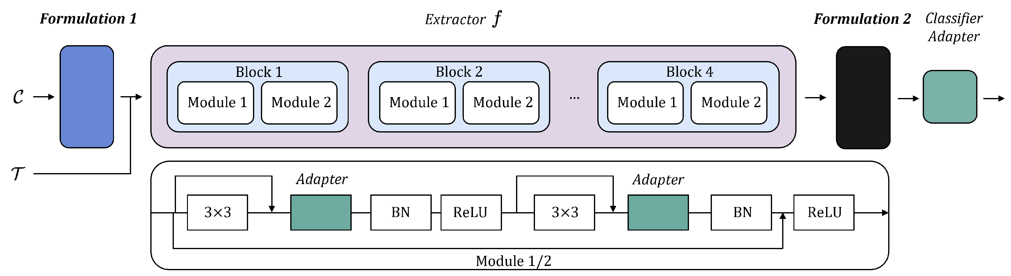
3.1.1. Formulation (1), Directly Resampling Task-Representation from Generative Density

Consider w as a deterministic function. Our first formulation adds a global sampling on the aggregate r. With this in mind, the procedure in Figure 3 indirectly forces a generative constraint to estimate the density p ( r ) with a local variational inference. Here, we amortize a portion of ϕ (as a reminder, f ( ; ϑ , ϕ ) ) using a conditional variational auto-encoder [39], where an encoder–decoder pair is jointly trained to approximate the conditional density function p ( r | r c ) , using estimated r c : = 1 / | C c | · x C c w ( x ) and, likewise, r : = ρ · w ( x C ) . That is, q ϑ is the encoder that takes duplicated and concatenated input to reparameterize a Gaussian distribution over the introduced latent z with its associated means μ z and variance Σ z ; and p ϑ 2 is the decoder to resample a r from the mean of each conditional distribution p ( r | r c , z ) .
In a latent variable perspective, we always sample from the generative density p ( r | r c ) in the highest probability, making the variables r easy to populate. This satisfies our representative purpose. In later optimization, we follow the variational inference to draw a log-likelihood lower bound to capture conditional density p ( r | r c ) . It assumes variable z to have a relaxed Gaussian prior p ( z ) = N ( 0 , I ) .

3.1.2. Formulation (2), a Resample Embedding Function from Grid Density

The second formulation considers a distribution over functions and places w p ( w ) into aggregating r : = ρ · ( w ( x C , y C ) ) . Considering, in 2D image regression, that a colored image corresponds to a mapping from an actual 2D grid location x i to its RGB pixel intensity y i R 3 , each latent feature map ν ( x ( c ) ) R d × h × e can be equivalently interpreted as an instance function from a stochastic process. Here, we apply the same manipulation as in Section 3.1.1 (but instead denoted as ν ) to first include the latent version of C .
Then, we can specify a function instance w on a fixed h × e grid [23,40]. Through reconstruction on each feature map, the target representation r can be bound to all the realizations p ( w ) . For illustration, we refer m : = ν ( x ) , x C to latent feature maps and n R h × e , the absolute position of the entries that constitutes m, to each 2D array. Further, we randomly select 2D indices to gather a (sub-)context-set M c and target-set M from all input pairs ( n , m ) , and approximating p ( w ) through predicting M by given M c . M c M is of note. The following parameterization is left for the Attentive Neural Processes (ANPs) [32], a latent collection of the Neural Process Family, with multi-head cross-attention [41,42,43] to predict the target-set feature maps.
The introduced model of ANPs has two branches featuring deterministic and latent properties, respectively. From Figure 4, a well-developed attention mechanism reformulates local encodings (i.e., the values) into representation r d in the deterministic path. It allows a given target location n ( t ) (query) to attend the location of the relevant context (i.e., the keys) in M c and to encode the dot-product relations. The latent path instead samples a variational latent z that captures distribution properties for subsequent prediction on grid values. We denote the overall parameterization as ϑ . These fixed dimension representations model a global structure of stochastic process realization, whereas r d in the deterministic path models is a fine-grained structure. Finally, a decoder takes representations [ z ; r d ] from the two paths generating grid density p ϑ ( m | n , z ; r d ) to estimate the final M . Aggregation of r : = ρ ( m · p ϑ ( m | n , z ; r d ) ) makes the representative vector of R d .
Theoretically, when p ϑ ( m ( t ) | n ( t ) , z ; r d ) specifies a Gaussian density characterized by respective [ μ ( t ) , σ 2 ( t ) ] to present each grid value, the factorization (see Section 2.2) goes into an infinite mixture of Gaussians:
p θ ( y T | x T ; C ) = p θ ( z | C ) t = 1 | T | N ( y ( t ) ; μ ( t ) , σ 2 ( t ) ) d z ,
meaning that the predictive distribution p ( w ) conceptually allows us to scale the complex likelihood function to diversify the global features. Our implementation additionally considers an experimental manipulation to reduce test-time complexity. That is, aggregating r solely on prototypes m ¯ and their reconstruction, while interpolation on 2D grid features is left for regularization. For each class k, the prototype is simply:
m ¯ k = 1 / | C k | · c = 1 | C k | ν ( x ( c ) ) .

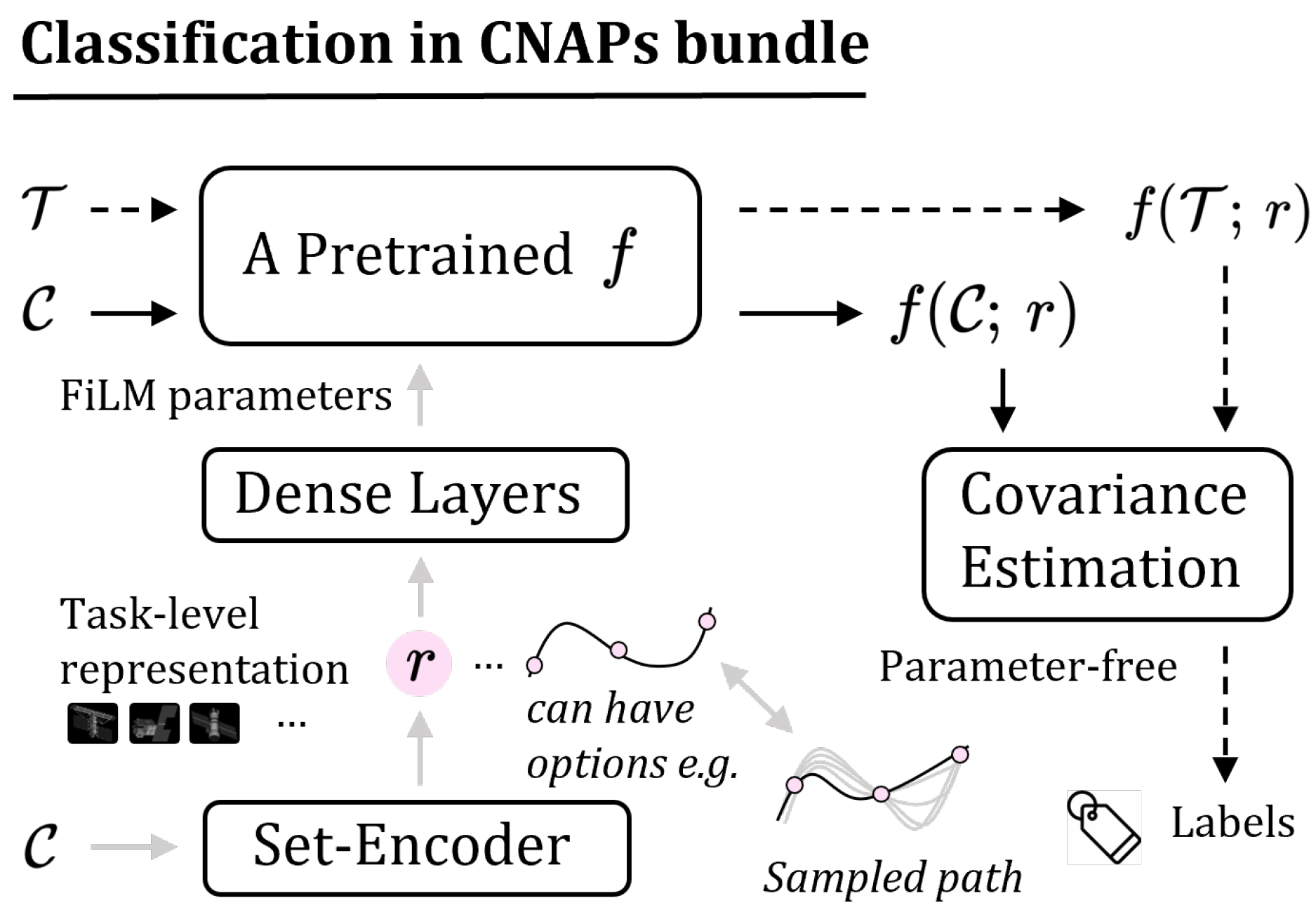
3.2. Building Estimated Classifier

To classify the adapted features of unlabeled targets, a non-parametric version of CNAPs [29] introduces a convex combination λ k · Σ k + 1 λ k · Σ into estimating covariance matrix Q k in the squared Mahalanobis distance for label k:
d k f x , x ¯ k = f x x ¯ k T Q k 1 f x x ¯ k .
Mathematically, each covariance estimation in the combination is dealt with using a sample covariance matrix; an unbiased and efficient estimator of the covariance matrix in this case. We first derive x ¯ k : = 1 / | C k | · x C k f x for class k and task-level prototype x ¯ : = 1 / | C | · x C f x . Then, by definition, each sample covariance relies on the difference between each observation and the sample mean, i.e., for a class-related covariance matrix:
Σ k = 1 C k 1 x C k f ( x ) x ¯ k f ( x ) x ¯ k T .
Then, use observations x C that cover whole context set for task-related covariance matrix Σ . Combining two matrices and considering all individual distributions in the task, the full covariance estimation presents a hierarchical regularization scheme [44]. Finally, the conditional predictive model finalizes its factorization assumption with an adapted embedding function f in a probabilistic mixture model [45], directly estimating the below likelihood function:
p y = k | f x ; C = e x p d k f x , x ¯ k k e x p d k f x , x ¯ k .
And, maximizing the correct likelihood helps to classify image x in T . Notice that Equation (15) is deterministic and exclusively dependent on the distribution over embedding function f, which is the key to our formulation below. Furthermore, the parameter-free structure with the squared Mahalanobis distance explores the theoretical properties of Bregman divergences well. The family of distance functions suggests a minimal distance in a softmax classifier from the sample as prototypes of all assigned data points.
There remains one downside to note: the above formulations and their classifier structure see deficiencies in generalizing out-of-distribution regimes, since true P ( D ) is still hard to cover. One of the strongest recommendations is to let ( C , T ) P ( D ) be a diverse dataset preparation for maximum-likelihood training. There then lies the top priority to digest diverse data, e.g., all training sources from BUAA [16] and the Meta-dataset [20] in joint training sessions.

3.3. Training Objects

Let p θ ( y T | x T ; C ) correspond to use of the parametric model θ to obtain a joint categorical distribution. In general, the target is to sample f for each task ( C , T ) and participate in classifying target images T into known labels from C . Now that the classifier is deterministic, Equation (15) can be directly maximized through episodic training with the associated classification dataset. Furthermore, we simultaneously summarize such episodic training into solving below local and global optimization.
In the local part, our first formulation instantiates the variational lower bound with an approximate KL divergence D K L , as well as an expectation that forms a log-likelihood lower bound L 1 ( ϑ ; C ) to have log p ( r | r c ) maximized:
L 1 ( ϑ ; C ) = D K L + E z q ϑ 1 ( z | r c , r ) log p ϑ 2 ( r | r c , z ) s . t . D K L = K L ( q ϑ 1 ( z | r c , r ) | | p ( z ) ) .
And, by definition, an encoder–decoder pair (parameterized by ϑ ) is used for approximating the true posterior q ( z | r c , r ) and conditional density p ( r | r c , z ) . Alternatively, our second inference principle is neural process variational inference [23]. The target objective evaluates learning the task-level representation r by applying Equation (8) to the Evidence Lower Bound (ELBO), specifically for embeddings of contexts C . During training, we infer latent variable z on a posterior sampling from p ϑ ( z | M ) , maximizing the lower-bound L V I ( ϑ ; M ) to predict latent feature maps:
L V I ( ϑ ; M ) = E z p ϑ ( z | M ) log t = 1 | M | p ϑ ( m ( t ) | n ( t ) , z ) K L p ϑ ( z | M ) p ϑ ( z | M c ) ,
where M and M c denote context-set and target-set. Not to confuse image–label pairs, here we use n to refer to 2D grid coordinates and m to refer to feature maps. To the best of our knowledge, we consider Equation (16), which takes advantage of whole C in a feasible objective, to meta-learn representations for the downstream task of adapting f. Essentially, we expect the model to reconstruct targets while being regularized by a fine-grained exploration within their structures.
Globally, in the maximum likelihood part, we have log-likelihood function specified to each classification dataset ( C , T ) instead. Furthermore, eventually, we evaluate the expected log-likelihood L ^ ( θ ; C , T ) on all those accessible tasks, approximately over distribution P ( C , T ) :
L ^ ( θ ; C , T ) = E ( C , T ) P ( C , T ) log p θ ( y T | x T ; C ) .
With reference to the provided pseudocode (see Algorithm 1), we repeat sampling ( C , T ) with image–label pairs and maximize Equation (18) in three steps: (1) learning from the given observation set C , (2) evaluating targets T , and (3) applying a gradient step until training converges.

3.4. Architecture with Formulation

In this paper, we first summarize the overall architecture into a local encoder–decoder pair and global encoder–decoder structure of Simple CNAPs, such that the encoder–decoder definition is consistent with the framework defined in the Neural Processes Family [23].
Specific choices of the local auxiliary architecture highly connect to the training objects. Behind the symbol ϕ , the first introduced is a conditional auto-encoder structure. Basically, the encoder part involves 4 convolutional layers, each followed by their own batch normalization and ReLU function that locally encodes category-wise sample means r c and the raw r into a predictive mean and a diagonal variance, implementing the reparameterization trick (with two individual linear layers) under a latent variable assumption [39] of a multivariate Gaussian distribution over each latent variable z, while the decoder part organizes subsequent 3 transposed convolutional blocks, with each LeakyReLU and a final Sigmoid activation on the top, to encourage our global resampling from the generative distribution p ( r | z , r c ) . Likewise, the second parameterization indicated with a latent neural process structure [23] involves 3 convolutional layers and their ReLU activations in its deterministic encoder E n c 1 , which locally encodes each concatenation [ n ( c ) , m ( c ) ] into r ( c ) . A two-head cross-attention layer with linear embedding functions follows behind. The latent encoder E n c 2 comprises the same amount of convolutional blocks, but is followed by 2 linear layers to reparameterize a latent posterior as in a VAE model [37]. Instead, the conditional decoder D e c takes 3 transposed convolutional layers and ReLUs together with linear layers (familiarly, a predictive mean and a diagonal variance function) to predict multivariate Gaussians, which each instance function w can be resampled from. A mean aggregator follows to take all realizations w p ( w ) into task-level representation r. Note that all the hidden representations will be of 128 dimensions.
Algorithm 1: Example Maximum Likelihood Training for Simple CNAPs
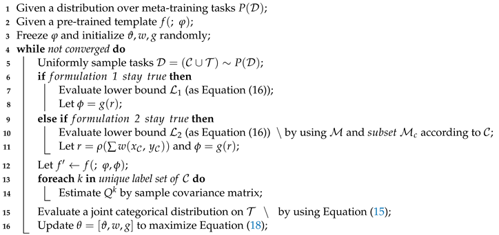
Remotesensing 15 04321 i001
Regarding the global structure, the encoder only requires us to produce task-level representation r and can be one of the two formulations above; the decoder is simply the ResNet-18 and a few amortization steps to generate plug-in FiLM layers [26]. In those steps, stacks of linear blocks map the aggregate representation r into those parameters of the channel-wise transformation, specifying the final adapted version f .
We apply the formulation to a new model: Task-Specific Adapters (TSAs) [46]. From Figure 5, TSAs are used for cross-domain few-shot classification that aims to learn a classifier from previously unseen classes and domains with few labeled samples. TSAs are commonly used with Universal Representation Learning (URL) [47], a single universal network learned and distilled from the labeled context set C. Briefly speaking, a TSA adapts the feature extractor created by URL using task-specific adapters. In this paper, we consider methods (Formulations (1) and (2)) in Section 3.1 as the pre-processed formulation and post-processed formulation, respectively.

4. Experiments

We first detail the Experimental setups in Section 4.1 and Section 4.2. Following comparisons in the BUAA dataset (see Section 4.3.1), we choose a simple distance-based learner D2N4 [4] that features adding image global pooling information into each feature descriptor, and our baseline Simple CNAPs [29], and the optimization-based learner, as the selected models.

4.1. Dataset Format

We evaluated our approach on the joint dataset, which is composed of the BUAA and the Meta-Dataset [20]. The Meta-Dataset is a large few-shot learning benchmark and consists of multiple datasets of different data distributions that feature 10 existing classification problems to help with anxiety. From Figure 6, the benchmark collects labeled data on diverse domains, varying from natural images with 1000 categories in ImageNet (ILSVRC-2012), FGVC-Aircraft (aircraft), QuickDraw (hand-drawn sketches), VGG Flower (flower images), FGVCx Fungi (mushroom), Omniglot (hand-written characters), CUB-200-2011 (birds), Describable Textures (texture), Traffic Signs, and MSCOCO (nature images). For any algorithm, samples from the first eight and the name of in-distribution tasks should not have overlapped during training, validation, and final testing. The unseen out-of-distribution split, instead, holds the combination of Traffic Signs, MSCOCO and held-out MNIST, CIFAR10, and CIFAR100. The algorithm should take them only for testing. BUAA, a space target dataset, has collected 20 classes of satellite models of different types, shapes, and functions. It is based on a space target 3-D model, using 3Ds MAX software to generate a space target full viewpoint simulation image. The data set consists of 4600 gray images from 230 viewpoints sampled on a viewing sphere, so each class has 230 examples. We adopt average accuracy and rank as the evaluation metric in our experiments. Considering the model’s rank makes it possible to obtain a more complete picture of its generalization performance, ensuring that the model remains stable and performs well under different data distributions and characteristics.

4.2. Implementation Details

4.2.1. Dataset Setting

To investigate the applicability of our scheme, we partitioned the BUAA dataset by placing 25% to 70% of the data categories (with a 5% gradient increase) inside the distribution and placing the remaining data categories outside the distribution. In our experiments, we only trained on the in-distribution data and used the out-of-distribution data for testing. In below sections, performance at each percentage accuracy will be reported by averaging over 600 proxy classification tasks with a 95% confidence interval. The benchmark setting does not restrict few-shot tasks to have fixed ways and shots, thus representing a more realistic scenario.

4.2.2. Training

In Section 3.1.2, we highlighted global sampling in latent neural process models, where the encoder, as the inference network, plays a dual role [23] of being an approximate posterior p ϑ ( z | M ) , and also of defining the prior, having observed M c , suggesting different behaviors in between stages: during training, we sample function instances from the approximate posterior when we have whole M in observation; during inference, instead, the sampling can only turn to the prior p ϑ ( z | M c ) given a subset of entries each feature map. We train an overall θ with 110,000 sampled tasks, using a task batch of 16 on all training splits from the Meta-dataset [20]. Our maximum likelihood training remains identical to [29] as we use episodic context/target splits C , T and set the size of all x within to be 84 × 84. A step learning rate (from 1 × 10 3 ) scheduler is set to configure the Adam optimizer. The whole procedure is loaded on a single NVIDIA RTX 3090 GPU.

4.3. Results and Extendable Discussion

We first report selected modelings on the BUAA dataset. However, before we discuss the benchmark part, we would like to demonstrate the potential of our proposal formulations in Section 3.1. As Section 2.2 explains, the task-level representation r plays an important role in the Conditional Neural Processes model. The proposal Formulations (1) and (2) are designed for this representation. However, we conclude that these formulations are generally applicable to the neural feature learning problem.
Notice the “test-only” setting means Table 2 evaluating spacecraft images as an out-of-distribution dataset. It can set a vital criterion to examine the model’s capacity to generalize unseen domains with public in-distribution examples. Then, we present a leaderboard on the Meta-Dataset to read how generalizable the models are in close-to-realistic applications.

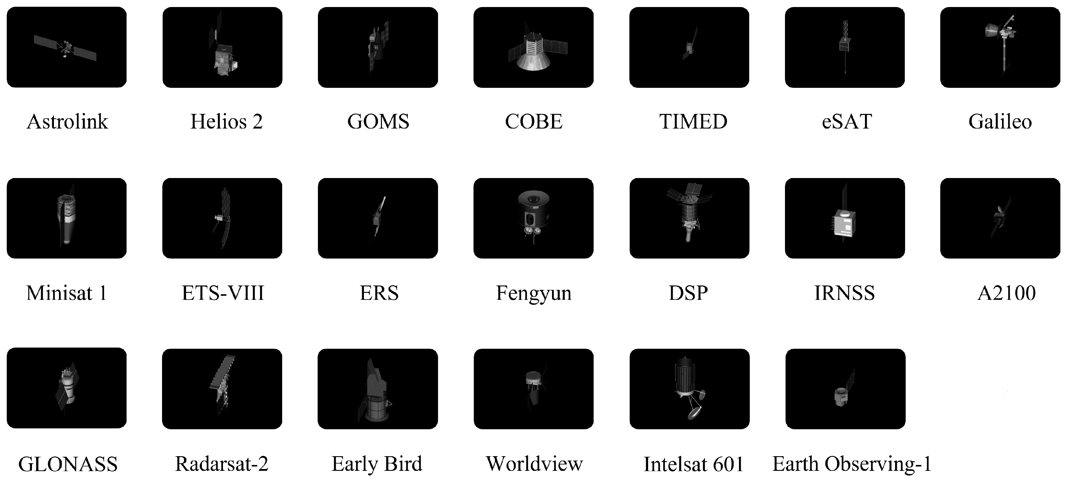
4.3.1. Benchmarking Spacecraft Dataset

The validation configures two different settings, and we would suggest a “single-domain training session” and “multi-domain joint training session”.
The setting of the first part adopts BUAA dataset as the only training data. Table 1 is more likely to represent the basic capacity of the baseline models when we exclude large-scale dataset and train models with our target domain data only. This can also help to ablate our later max likelihood training. As shown, an average rank via aggregating across each column of Table 1 both suggests baseline TSA and Simple CNAPs outperform the simple distance learner D2N4; the modification on TSA encourages its capacity when having nearly at least half percent available training data. A more intuitive demonstration can refer to Figure 7a, where all the conditional models maintain an upward performance if expanding the training splits, but a similar conclusion does not hold for D2N4.
The setting of the second part adopts all accessible datasets as the training data instead. Furthermore, what Table 2 conveys is that both of our formulations turn more competitive in a joint maximum likelihood modeling with all training splits of the Meta-Dataset included; particularly, the second formulation prominently leads the result. From a direct comparison between Figure 7a,b, a wide range of cross-domain training also benefits the distance-based learner, while some cases see declines for Simple CNAPs. An interesting result can also be found in the test-only case (Table 2) and a proportion of 70% categories used in training (Table 1). The result of our formulation using only BUAA for testing in Table 2 is even comparable to the result of D2N4 in Table 1 using the 70% of samples used in training. Modifications on TSA convey such improvement, too, making them the highest average rank among the listed methods. However, such an advantage becomes less when Simple CNAPs∼fo. 2 makes a well-matched competition with at least 60% of available training categories.

4.3.2. Benchmarking Meta-Dataset

The validation in this subsection goes into two different settings, and we would suggest a “leaderboard version of unseen tasks performance” and “joint-training version of unseen tasks performance”.
The first part sees models trained at all available datasets of the Meta-Dataset and tested on it. Table 3 and Table 4 display the in/out-of-distribution statuses for benchmark models. This setting, however, excludes the BUAA dataset and makes spacecraft images test-only (the source of that column in Table 2). In Table 3, we also compare methods with the unseen parts of training sources. The universal representation approach, i.e., SUR [12] and URT [13], achieves classification by training a respective embedding function for each intra-distributed dataset and then linearly combining each embedding function to form a specific embedding function based on the task query set. However, a considerable domain gap against training sources in out-of-distribution settings explains their need to be more generalizable from the eight extractors. Instead, we are motivated to approximate a distribution over dataset-specified embedding functions for Simple CNAPs and to sample the proper one for each test-time task, which is more efficient [24]. Modifications of TSAs convey such an idea too. Further evidence of a comparable average rank among listed models shows our meta-learned formulations promote feature adaptation over the same embedding function as in Simple CNAPs. Another promising result would be the highest average rank for TSA∼fo. 1 in Table 4, where we generalize all models to the out-of-distribution splits of Meta-Dataset. Generative formulation 1 extends the embedding extractor function of Simple CNAPs and TSAs from encoding static training datasets only to having generative density, such that resampling schemes can efficiently encourage adapting out-of-distribution tasks.
The second part is attached to the “multi-domain joint training session” of Section 4.3.1, where the setting instead evaluates the incorporation of spacecraft images into Meta-Dataset performance. Figure 7c,d represent in- and out-of-distribution splits of the Meta-Dataset, respectively. Similar to spacecraft images, cases of Simple CNAPs on the auxiliary Meta-Dataset suggest a sharp drop, indicating a deterministic representation in the conditional model is less likely to adapt more domains than the stochastic one. Fewer side effects can be found with all our modifications, suggesting a potential capability to continue to learn data from a new domain (at least for spacecraft images).

4.4. Ablation Study

By analyzing Table 1 and Table 2, it can be seen that the recognition accuracy of the target domain can be improved dramatically when using the joint data as the auxiliary data of the target domain. The effect is significant, even if the target domain is not used in the training phase.
Since space target images have large intra-class gaps and small inter-class gaps and are close to fine-grained classification settings, we use a classifier based on Mahalanobis distance to improve classification performance by analyzing the overall and local variance. Table 5 shows that the Mahalanobis distance outperforms the Euclidean distance when only the space target image is used for testing. However, when the amount of space target data is increased during training, the performance of both is almost equal. This is because as the number of training samples in the target domain increases, the learnable feature extractor can achieve the optimization of the intra-class distribution, which reduces the effect of the Mahalanobis distance.

5. Conclusions and Limitations

This paper uses conditional variational inference and latent neural processes [32] to learn diversified representations over multiple datasets while generalizing spacecraft recognition to a generalization problem to improve space target recognition performance with the aid of multi-domain datasets. On optimizing Equation (4), we propose to condition such meta-learned task-level representations on feature adaptation; as a result, the promoted adaptation of Simple CNAPs and TSAs improves their performance for benchmark classification for the spacecraft images both in-distribution and out-of-distribution. The algorithm also shows competitive results on larger benchmark settings for multitasking or versatility purposes. Similar conclusions still hold when we extend the feature learning to a more general stage, where the proposed formulation preprocesses and post-processes. The algorithm also shows competitive results on a larger benchmark setting for multi-task purposes. Our approach starts from representation and solves the few-shot problem by generalizing the prototypical representation of the target data, so it has a strong generalization ability for the domains where data acquisition is expensive, such as medical engineering and ocean observations [49]. However, BUAA dataset lacks light intensity variations as well as stellar interference compared to real space target images, and further validation of the model will be performed when the real data is complete. Our experiments also suggest a catastrophic interference, as all the modifications end up forgetting the Meta-dataset training after including spacecraft images with the joint training. A possible future work approach is extending our rough applications of neural processes to support future learning.

Author Contributions

Methodology, X.Y. and D.Y.; Software, D.K. and R.L.; Formal analysis, D.K.; Data curation, D.K.; Writing—original draft, X.Y. and R.L.; Writing—review & editing, D.Y.; Supervision, D.Y. All authors have read and agreed to the published version of the manuscript.

Funding

National Natural Science Foundation of China: 62372348, 61976166; Shaanxi Outstanding Youth Science Fund Project: 2023-JC-JQ-53; Fundamental Research Funds for the Central Universities: QTZX23057; Open Research Projects of Laboratory of Pinghu.

Conflicts of Interest

The authors declare no conflict of interest.

References

  1. Zhao, Z.; Xu, G.; Zhang, N.; Zhang, Q. Performance analysis of the hybrid satellite-terrestrial relay network with opportunistic scheduling over generalized fading channels. IEEE Trans. Veh. Technol. 2022, 71, 2914–2924. [Google Scholar] [CrossRef]
  2. Heidari, A.; Jafari Navimipour, N.; Unal, M.; Zhang, G. Machine learning applications in internet-of-drones: Systematic review, recent deployments, and open issues. ACM Comput. Surv. 2023, 55, 1–45. [Google Scholar] [CrossRef]
  3. Zeng, H.; Xia, Y. Space target recognition based on deep learning. In Proceedings of the 2017 20th International Conference on Information Fusion (Fusion), Xi’an, China, 10–13 July 2017. [Google Scholar]
  4. Yang, X.; Nan, X.; Song, B. D2N4: A Discriminative Deep Nearest Neighbor Neural Network for Few-shot Space Target Recognition. IEEE Trans. Geosci. Remote Sens. 2020, 58, 3667–3676. [Google Scholar] [CrossRef]
  5. Peng, R.; Zhao, W.; Li, K.; Ji, F.; Rong, C. Continual Contrastive Learning for Cross-Dataset Scene Classification. Remote Sens. 2022, 14, 5105. [Google Scholar] [CrossRef]
  6. Gordon, J.; Bronskill, J.; Bauer, M.; Nowozin, S.; Turner, R. Meta-Learning Probabilistic Inference for Prediction. In Proceedings of the International Conference on Learning Representations, New Orleans, LA, USA, 6–9 May 2019. [Google Scholar]
  7. Chen, W.Y.; Liu, Y.C.; Kira, Z.; Wang, Y.C.F.; Huang, J.B. A Closer Look at Few-shot Classification. In Proceedings of the International Conference on Learning Representations, New Orleans, LA, USA, 6–9 May 2019. [Google Scholar]
  8. Rostami, M.; Kolouri, S.; Eaton, E.; Kim, K. Deep transfer learning for few-shot SAR image classification. Remote Sens. 2019, 11, 1374. [Google Scholar] [CrossRef]
  9. Bai, X.; Huang, M.; Xu, M.; Liu, J. Reconfiguration Optimization of Relative Motion between Elliptical Orbits Using Lyapunov-Floquet Transformation. IEEE Trans. Aerosp. Electron. Syst. 2022, 59, 923–936. [Google Scholar] [CrossRef]
  10. Yang, S.; Liu, L.; Xu, M. Free Lunch for Few-shot Learning: Distribution Calibration. In Proceedings of the International Conference on Learning Representations, Online, 26–30 April 2020. [Google Scholar]
  11. Huang, W.; Yuan, Z.; Yang, A.; Tang, C.; Luo, X. TAE-net: Task-adaptive embedding network for few-shot remote sensing scene classification. Remote Sens. 2022, 14, 111. [Google Scholar] [CrossRef]
  12. Dvornik, N.; Schmid, C.; Mairal, J. Selecting Relevant Features from A Universal representation for few-shot classification. In Proceedings of the European Conference on Computer Vision, Glasgow, UK, 29 September–4 October 2020. [Google Scholar]
  13. Liu, L.; Hamilton, W.; Long, G.; Jiang, J.; Larochelle, H. A Universal Representation Transformer Layer for Few-Shot Image Classification. In Proceedings of the International Conference on Learning Representations, Vienna, Austria, 4–8 May 2021. [Google Scholar]
  14. Finn, C.; Abbeel, P.; Levine, S. Model-Agnostic Meta-Learning for Fast Adaptation of Deep Networks. In Proceedings of the International Conference on Machine Learning, Sydney, Australia, 11–158 August 2017. [Google Scholar]
  15. Triantafillou, E.; Larochelle, H.; Zemel, R.; Dumoulin, V. Learning a Universal Template for Few-shot Dataset Generalization. In Proceedings of the International Conference on Machine Learning, Online, 18–24 July 2021. [Google Scholar]
  16. Zhang, H.; Liu, Z.; Jiang, Z.; An, M.; Zhao, D. BUAA-SID1.0 Space object Image Dataset. Spacecr. Recovery Remote Sens. 2010, 31, 65–71. [Google Scholar]
  17. Wang, Y.; Yao, Q.; Kwok, J.T.; Ni, L.M. Generalizing from A Few Examples: A Survey on Few-shot Learning. ACM Comput. Surv. 2020, 53, 1–34. [Google Scholar] [CrossRef]
  18. Williams, C.K.; Rasmussen, C.E. Gaussian Processes for Machine Learning; MIT Press: Cambridge, UK, 2006. [Google Scholar]
  19. Ravi, S.; Larochelle, H. Optimization as A Model for Few-shot Learning. In Proceedings of the International Conference on Learning Representations, San Juan, PR, USA, 2–4 May 2016. [Google Scholar]
  20. Triantafillou, E.; Zhu, T.; Dumoulin, V.; Lamblin, P.; Evci, U.; Xu, K.; Goroshin, R.; Gelada, C.; Swersky, K.; Manzagol, P.A.; et al. Meta-dataset: A Dataset of Datasets for Learning to Learn from Few Examples. In Proceedings of the International Conference on Learning Representations, Online, 26–30 April 2020. [Google Scholar]
  21. Russakovsky, O.; Deng, J.; Su, H.; Krause, J.; Satheesh, S.; Ma, S.; Huang, Z.; Karpathy, A.; Khosla, A.; Bernstein, M.; et al. Imagenet Large Scale Visual Recognition Challenge. Int. J. Comput. Vis. 2015, 115, 211–252. [Google Scholar] [CrossRef]
  22. Lin, T.Y.; Maire, M.; Belongie, S.; Hays, J.; Perona, P.; Ramanan, D.; Dollár, P.; Zitnick, C.L. Microsoft COCO: Common Objects in Context. In Proceedings of the European Conference on Computer Vision, Zurich, Switzerland, 6–12 September 2014. [Google Scholar]
  23. Garnelo, M.; Schwarz, J.; Rosenbaum, D.; Viola, F.; Rezende, D.J.; Eslami, S.; Teh, Y.W. Neural Processes. arXiv 2018, arXiv:1807.01622. [Google Scholar]
  24. Requeima, J.; Gordon, J.; Bronskill, J.; Nowozin, S.; Turner, R.E. Fast and Flexible Multi-task Classification Using Conditional Neural Adaptive Processes. In Proceedings of the Advances in Neural Information Processing Systems, Vancouver, QC, Canada, 8–14 December 2019. [Google Scholar]
  25. Garnelo, M.; Rosenbaum, D.; Maddison, C.; Ramalho, T.; Saxton, D.; Shanahan, M.; Teh, Y.W.; Rezende, D.; Eslami, S.A. Conditional Neural Processes. In Proceedings of the International Conference on Machine Learning, Stockholm, Sweden, 10–15 July 2018. [Google Scholar]
  26. Perez, E.; Strub, F.; De Vries, H.; Dumoulin, V.; Courville, A. Film: Visual reasoning with a general conditioning layer. In Proceedings of the AAAI Conference on Artificial Intelligence, New Orleans, LA, USA, 2–7 February 2018. [Google Scholar]
  27. Petersen, J.; Köhler, G.; Zimmerer, D.; Isensee, F.; Jäger, P.F.; Maier-Hein, K.H. GP-ConvCNP: Better Generalization for Conditional Convolutional Neural Processes on Time Series Data. In Proceedings of the Thirty-Seventh Conference on Uncertainty in Artificial Intelligence, Online, 27–29 July 2021. [Google Scholar]
  28. He, K.; Zhang, X.; Ren, S.; Sun, J. Deep Residual Learning for Image Recognition. In Proceedings of the IEEE/CVF Conference on Computer Vision and Pattern Recognition, Las Vegas, NV, USA, 26 June–1 July 2016. [Google Scholar]
  29. Bateni, P.; Goyal, R.; Masrani, V.; Wood, F.; Sigal, L. Improved Few-shot Visual Classification. In Proceedings of the IEEE/CVF Conference on Computer Vision and Pattern Recognition, Seattle, WA, USA, 13–19 June 2020. [Google Scholar]
  30. Zaheer, M.; Kottur, S.; Ravanbakhsh, S.; Poczos, B.; Salakhutdinov, R.R.; Smola, A.J. Deep Sets. In Proceedings of the Advances in Neural Information Processing Systems, Long Beach, CA, USA, 4–9 December 2017. [Google Scholar]
  31. Cremer, C.; Li, X.; Duvenaud, D. Inference Suboptimality in Variational Autoencoders. In Proceedings of the International Conference on Machine Learning, Stockholm, Sweden, 10–15 July 2018. [Google Scholar]
  32. Kim, H.; Mnih, A.; Schwarz, J.; Garnelo, M.; Eslami, A.; Rosenbaum, D.; Vinyals, O.; Teh, Y.W. Attentive Neural Processes. In Proceedings of the International Conference on Learning Representations, New Orleans, LA, USA, 6–9 May 2019. [Google Scholar]
  33. Andrychowicz, M.; Denil, M.; Gomez, S.; Hoffman, M.W.; Pfau, D.; Schaul, T.; Shillingford, B.; De Freitas, N. Learning to Learn by Gradient Gescent by Gradient Descent. In Proceedings of the Advances in Neural Information Processing Systems, Barcelona, Spain, 5–10 December 2016. [Google Scholar]
  34. Snell, J.; Swersky, K.; Zemel, R. Prototypical Networks for Few-shot Learning. In Proceedings of the Advances in Neural Information Processing Systems, Long Beach, CA, USA, 4–9 December 2017. [Google Scholar]
  35. Zeng, Q.; Geng, J.; Huang, K.; Jiang, W.; Guo, J. Prototype calibration with feature generation for few-shot remote sensing image scene classification. Remote Sens. 2021, 13, 2728. [Google Scholar] [CrossRef]
  36. Nichol, A.; Achiam, J.; Schulman, J. On First-order Meta-learning Algorithms. arXiv 2018, arXiv:1803.02999. [Google Scholar]
  37. Kingma, D.P.; Welling, M. Auto-encoding variational bayes. In Proceedings of the International Conference on Learning Representations, Banff, AB, USA, 14–16 April 2014. [Google Scholar]
  38. Ghahramani, Z. Probabilistic Machine Learning and Artificial Intelligence. Nature 2015, 521, 452–459. [Google Scholar] [CrossRef] [PubMed]
  39. Sohn, K.; Lee, H.; Yan, X. Learning Structured Output Representation Using Deep Conditional Generative Models. In Proceedings of the Advances in Neural Information Processing Systems, Montreal, QC, Canada, 11–12 December 2015. [Google Scholar]
  40. Gordon, J.; Bruinsma, W.P.; Foong, A.Y.K.; Requeima, J.; Dubois, Y.; Turner, R.E. Convolutional Conditional Neural Processes. In Proceedings of the International Conference on Learning Representations, Online, 26–30 April 2020. [Google Scholar]
  41. Vaswani, A.; Shazeer, N.; Parmar, N.; Uszkoreit, J.; Jones, L.; Gomez, A.N.; Kaiser, Ł.; Polosukhin, I. Attention is All You Need. In Proceedings of the Advances in Neural Information Processing Systems, Long Beach, CA, USA, 4–9 December 2017. [Google Scholar]
  42. Zhang, H.; Luo, G.; Li, J.; Wang, F.Y. C2FDA: Coarse-to-fine domain adaptation for traffic object detection. IEEE Trans. Intell. Transp. Syst. 2021, 23, 12633–12647. [Google Scholar] [CrossRef]
  43. Zhao, K.; Jia, Z.; Jia, F.; Shao, H. Multi-scale integrated deep self-attention network for predicting remaining useful life of aero-engine. Eng. Appl. Artif. Intell. 2023, 120, 105860. [Google Scholar] [CrossRef]
  44. Gao, H.; Shou, Z.; Zareian, A.; Zhang, H.; Chang, S.F. Low-shot Learning via Covariance-Preserving Adversarial Augmentation Networks. In Proceedings of the Advances in Neural Information Processing Systems, Montreal, QC, Canada, 3–8 December 2018. [Google Scholar]
  45. Wang, Z.; Lan, L.; Vucetic, S. Mixture Model for Multiple Instance Regression and Applications in Remote Sensing. IEEE Trans. Geosci. Remote Sens. 2012, 50, 2226–2237. [Google Scholar] [CrossRef]
  46. Li, W.H.; Liu, X.; Bilen, H. Cross-domain Few-shot Learning with Task-specific Adapters. In Proceedings of the IEEE/CVF Conference on Computer Vision and Pattern Recognition, New Orleans, LA, USA, 21–24 June 2022. [Google Scholar]
  47. Li, W.H.; Liu, X.; Bilen, H. Universal Representation Learning from Multiple Domains for Few-shot Classification. In Proceedings of the IEEE/CVF International Conference on Computer Vision, Montreal, QC, Canada, 11–17 October 2021. [Google Scholar]
  48. Bateni, P.; Barber, J.; van de Meent, J.W.; Wood, F. Enhancing Few-Shot Image Classification with Unlabelled Examples. In Proceedings of the IEEE Workshop on Applications of Computer Vision, Snowmass Village, CO, USA, 4–8 January 2022. [Google Scholar]
  49. Yang, M.; Wang, Y.; Wang, C.; Liang, Y.; Yang, S.; Wang, L.; Wang, S. Digital twin-driven industrialization development of underwater gliders. IEEE Trans. Ind. Inform. 2023, 19, 9680–9690. [Google Scholar] [CrossRef]
Figure 1. Inspection of the BUAA dataset. The data generation uses 3D triangulated models with dark backgrounds, simulating aircraft in deep space. Images of each category are uniformly rendered from 230 viewpoints on a default view port in 3Ds MAX software.
Remotesensing 15 04321 g001
Figure 2. The “Simple” variant of Conditional Neural Adaptive Processes in few-shot classifications [29]. The model also follows the rules of a meta-learning algorithm that learns from labeled context-set ( C ) images and predicts unlabeled target-set images ( T ).
Remotesensing 15 04321 g002
Figure 3. Overview of Formulation (1): the resampling task representative of a latent distribution posterior reparamertized by a conditional variational inference.
Remotesensing 15 04321 g003
Figure 4. Overview of Formulation (2): resampling a latent embedding function in grid density. The pipeline is adapted from [32], except that we manipulate grid samples.
Remotesensing 15 04321 g004
Figure 5. Overview of reformulated Task-specific Adapters (TSAs). The TSA model adapts extractor distilled from the Universal Representation Learning (URL) technique. Here, we reformulate its preprocessing part.
Remotesensing 15 04321 g005
Figure 6. The datasets of the dataset, including the Meta-dataset’s 10 datasets and the left three datasets Mnist and Cifar10/100 for additional tests.
Remotesensing 15 04321 g006
Figure 7. Comparisons from (a,b) evaluate models trained on BUAA dataset only, and in similar settings, but instead with joint maximum likelihood training. (c,d) show performance on Meta-Dataset in-distribution/out-of-distribution testing using models trained with (none-zero x axis) or without (zero x axis) feeding spacecraft images.
Remotesensing 15 04321 g007
Table 1. Results reported on unseen in-distribution tasks of BUAA dataset using models trained on a single domain.
Avg. Rank25%.30%.35%.40%.45%.50%.55%.60%.65%.70% Categories
D2N4 [4]5.788.6 ± 0.789.9 ± 0.692.1 ± 0.590.8 ± 0.691.1 ± 0.692.1 ± 0.693.8 ± 0.594.5 ± 0.594.9 ± 0.493.9 ± 0.4
Simple CNAPs [29]2.092.9 ± 0.693.8 ± 0.594.4 ± 0.694.2 ± 0.693.9 ± 0.494.7 ± 0.695.0 ± 0.595.2 ± 0.696.3 ± 0.597.0 ± 0.4
TSA [46]3.093.6 ± 0.593.9 ± 0.594.4 ± 0.494.1 ± 0.594.3 ± 0.594.4 ± 0.494.7 ± 0.594.9 ± 0.396.1 ± 0.496.4 ± 0.3
Sim. CNAPs∼fo. 15.985.8 ± 0.788.7 ± 0.691.6 ± 0.591.5 ± 0.691.9 ± 0.790.2 ± 0.792.2 ± 0.694.7 ± 0.594.0 ± 0.597.0 ± 0.3
Sim. CNAPs∼fo. 25.188.0 ± 0.692.0 ± 0.591.1 ± 0.693.5 ± 0.691.6 ± 0.793.2 ± 0.593.8 ± 0.594.5 ± 0.694.5 ± 0.496.3 ± 0.3
TSA∼fo. 14.188.1 ± 0.489.6 ± 0.591.7 ± 0.692.4 ± 0.493.5 ± 0.494.6 ± 0.594.9 ± 0.495.0 ± 0.594.5 ± 0.596.1 ± 0.4
TSA∼fo. 22.190.4 ± 0.491.7 ± 0.693.0 ± 0.594.6 ± 0.495.4 ± 0.695.2 ± 0.595.7 ± 0.395.6 ± 0.496.8 ± 0.597.5 ± 0.4
Table 2. Results reported on joint In-distribution tasks of BUAA dataset using models trained on multiple domains.
Avg. RankTest Only25%.30%.35%.40%.45%.50%.55%.60%.65%.70% Categories
D2N4 [4]6.189.9 ± 0.690.3 ± 0.692.3 ± 0.593.8 ± 0.594.4 ± 0.594.7 ± 0.595.3 ± 0.495.8 ± 0.596.2 ± 0.496.3 ± 0.496.5 ± 0.4
Simple CNAPs [29]6.491.2 ± 0.793.2 ± 0.693.6 ± 0.694.0 ± 0.694.3 ± 0.694.0 ± 0.594.5 ± 0.694.1 ± 0.595.1 ± 0.696.0 ± 0.596.7 ± 0.5
TSA [46]4.194.2 ± 1.095.3 ± 0.795.7 ± 0.795.5 ± 0.695.8 ± 0.695.6 ± 0.795.8 ± 0.695.4 ± 0.796.0 ± 0.596.3 ± 0.696.5 ± 0.6
Sim. CNAPs∼fo. 14.392.6 ± 0.594.5 ± 0.495.2 ± 0.495.5 ± 0.595.4 ± 0.496.9 ± 0.495.6 ± 0.496.3 ± 0.496.8 ± 0.397.0 ± 0.397.4 ± 0.3
Sim. CNAPs∼fo. 23.393.1 ± 0.694.1 ± 0.594.9 ± 0.595.3 ± 0.495.8 ± 0.496.4 ± 0.396.8 ± 0.497.3 ± 0.497.5 ± 0.397.8 ± 0.498.2 ± 0.3
TSA∼fo. 11.795.2 ± 0.896.2 ± 0.696.6 ± 0.796.9 ± 0.697.3 ± 0.597.7 ± 0.597.6 ± 0.697.4 ± 0.697.6 ± 0.597.8 ± 0.497.9 ± 0.4
TSA∼fo. 22.094.4 ± 1.095.4 ± 0.595.9 ± 0.496.5 ± 0.596.4 ± 0.597.3 ± 0.397.8 ± 0.497.9 ± 0.497.6 ± 0.598.1 ± 0.498.4 ± 0.3
Table 3. Results reported on in-distribution tasks using models trained on all training datasets.
Avg. RankILSVRCOmniglotAircraftBirdsTexturesQuickDrawFungiFlower
D2N4 [4]15.326.1 ± 0.882.8 ± 0.972.8 ± 0.934.6 ± 1.052.7 ± 0.766.6 ± 0.932.3 ± 0.972.8 ± 0.8
fo-MAML [20]14.637.8 ± 1.083.9 ± 0.976.4 ± 0.762.4 ± 1.164.2 ± 0.859.7 ± 1.133.5 ± 1.180.0 ± 0.8
ProtoNet [34]14.344.5 ± 1.079.6 ± 1.171.1 ± 0.967.0 ± 1.065.2 ± 0.864.9 ± 0.940.3 ± 1.186.8 ± 0.7
Proto-MAML [20]12.646.5 ± 1.082.7 ± 1.075.2 ± 0.869.9 ± 1.068.2 ± 0.866.8 ± 0.942.0 ± 1.188.7 ± 0.7
CNAPs [24]11.151.0 ± 1.090.7 ± 0.672.3 ± 0.873.0 ± 0.854.8 ± 0.774.2 ± 0.650.2 ± 1.088.5 ± 0.6
Simple CNAPs [29]9.056.5 ± 1.091.7 ± 0.682.4 ± 0.774.9 ± 0.967.8 ± 0.777.5 ± 0.846.9 ± 1.089.7 ± 0.6
SUR [12]8.356.1 ± 1.193.1 ± 0.584.6 ± 0.770.6 ± 1.071.0 ± 0.881.3 ± 0.664.2 ± 1.182.8 ± 0.8
FLUTE [15]7.551.8 ± 1.093.2 ± 0.587.2 ± 0.579.2 ± 0.868.8 ± 0.879.5 ± 0.758.1 ± 1.191.6 ± 0.6
Transductive CNAPs [48]6.957.9 ± 1.194.3 ± 0.484.7 ± 0.578.8 ± 0.766.2 ± 0.877.9 ± 0.648.9 ± 1.292.3 ± 0.4
URT [13]6.755.7 ± 1.094.4 ± 0.485.8 ± 0.676.3 ± 0.871.8 ± 0.782.5 ± 0.663.5 ± 1.088.2 ± 0.6
URL [47]3.157.5 ± 1.194.5 ± 0.488.6 ± 0.580.5 ± 0.776.2 ± 0.781.8 ± 0.668.7 ± 1.092.1 ± 0.5
TSA [46]2.857.3 ± 1.095.0 ± 0.489.3 ± 0.481.4 ± 0.776.7 ± 0.782.0 ± 0.667.4 ± 1.092.2 ± 0.5
Simple CNAPs∼fo. 19.552.5 ± 1.188.2 ± 0.874.5 ± 0.873.2 ± 0.974.0 ± 0.880.5 ± 0.753.4 ± 1.190.2 ± 0.6
Simple CNAPs∼fo. 27.855.1 ± 1.192.2 ± 0.681.4 ± 0.678.1 ± 0.872.9 ± 0.980.4 ± 0.759.4 ± 1.089.7 ± 0.6
TSA∼fo. 14.054.1 ± 0.893.8 ± 0.685.8 ± 1.078.4 ± 1.080.1 ± 0.884.2 ± 0.868.7 ± 0.793.1 ± 0.8
TSA∼fo. 22.356.6 ± 0.696.4 ± 0.888.4 ± 0.583.1 ± 0.878.6 ± 1.084.4 ± 0.869.5 ± 1.092.8 ± 0.7
Table 4. Results reported on out-of-distribution tasks using models trained on all training datasets.
Avg. RankTraffic SignsMSCOCOMnistCifar10Cifar100
fo-MAML [20]15.842.9 ± 1.329.4 ± 1.1---
ProtoNet [34]14.346.5 ± 1.039.9 ± 1.0---
D2N4 [4]11.560.7 ± 1.128.2 ± 0.992.9 ± 0.544.0 ± 0.739.0 ± 1.0
Proto-MAML [20]11.252.4 ± 1.141.7 ± 1.1---
CNAPs [24]10.856.5 ± 1.139.4 ± 1.092.7 ± 0.461.5 ± 0.750.1 ± 1.0
SUR [12]10.053.4 ± 1.050.1 ± 1.094.3 ± 0.466.8 ± 0.956.6 ± 1.0
URT [13]9.651.1 ± 1.152.2 ± 1.194.8 ± 0.467.3 ± 0.856.9 ± 1.0
Simple CNAPs [29]9.259.2 ± 1.042.4 ± 1.193.9 ± 0.474.3 ± 0.760.5 ± 1.0
Transductive CNAPs [48]7.159.7 ± 1.142.5 ± 1.195.7 ± 0.375.7 ± 0.762.9 ± 1.0
FLUTE [15]6.658.4 ± 1.150.0 ± 1.095.6 ± 0.578.6 ± 0.767.1 ± 1.0
URL [47]6.763.3 ± 1.254.0 ± 1.094.7 ± 0.474.2 ± 0.863.5 ± 1.0
TSA [46]2.383.5 ± 0.955.7 ± 1.196.7 ± 0.482.9 ± 0.770.4 ± 0.9
Simple CNAPs∼fo. 16.469.5 ± 0.852.6 ± 0.793.6 ± 0.470.5 ± 0.869.0 ± 1.0
Simple CNAPs∼fo. 26.567.4 ± 1.055.3 ± 0.792.5 ± 0.568.4 ± 0.869.8 ± 0.9
TSA∼fo. 11.885.4 ± 0.858.7 ± 1.095.1 ± 0.681.5 ± 0.673.3 ± 0.8
TSA∼fo. 22.484.1 ± 0.656.6 ± 0.896.4 ± 0.680.3 ± 0.871.7 ± 0.7
Table 5. Results of different metrics in the classifier on BUAA.
Simple CNAPs [29]Simple CNAPs∼fo. 1Simple CNAPs∼fo. 2TSA [46]TSA∼fo. 1TSA∼fo. 2
Mahalanobis distance (test only)91.2 ± 0.792.6 ± 0.593.1 ± 0.694.2 ± 1.095.2 ± 0.594.4 ± 1.0
European distance (test only)90.7 ± 0.891.2 ± 0.492.4 ± 0.693.4 ± 0.894.5 ± 0.394.6 ± 0.9
Mahalanobis distance (70% for training)96.7 ± 0.597.4 ± 0.398.2 ± 0.396.5 ± 0.697.9 ± 0.498.4 ± 0.3
European distance (70% for training)96.6 ± 0.597.6 ± 0.597.9 ± 0.896.8 ± 0.397.7 ± 0.798.2 ± 0.6
Disclaimer/Publisher’s Note: The statements, opinions and data contained in all publications are solely those of the individual author(s) and contributor(s) and not of MDPI and/or the editor(s). MDPI and/or the editor(s) disclaim responsibility for any injury to people or property resulting from any ideas, methods, instructions or products referred to in the content.

