Article

Estimating Leymus chinensis Loss Caused by Oedaleus decorus asiaticus Using an Unmanned Aerial Vehicle (UAV)

1
Institute of Grassland Research, Chinese Academy of Agricultural Sciences, Hohhot 010010, China
2
Inner Mongolia Academy of Grassland Science, Hohhot 010010, China
3
North Agriculture and Livestock Husbandry Technology Innovation Center (NALHTIC), Chinese Academy of Agricultural Sciences, Hohhot 010010, China
4
Key Laboratory of Digital Earth Science, Aerospace Information Research Institute, Chinese Academy of Sciences, Beijing 100094, China
5
University of Chinese Academy of Sciences, Beijing 100049, China
*
Author to whom correspondence should be addressed.
Remote Sens. 2023, 15(17), 4352; https://doi.org/10.3390/rs15174352
Submission received: 10 July 2023 / Revised: 1 September 2023 / Accepted: 2 September 2023 / Published: 4 September 2023

Abstract

:
Oedaleus decorus asiaticus is one of the dominant harmful pests in central Inner Mongolia, China. Large-scale outbreaks of this pest create many serious problems in animal husbandry and agriculture. Therefore, understanding the underlying mechanisms between plant losses and Odecorus at different density levels and growth stages can guide the development of monitoring and prediction measures to reduce damage. In this study, an unmanned aerial vehicle (UAV) carrying a camera was employed to collect multi-spectral data. Further, nine vegetation indices (VIs) were analyzed to explore the most suitable indices for estimating plant loss caused by O. decorus in different growth stages. The following results were obtained: (1) The second instar nymphs of O. decorus could promote vegetation growth. As the density level in each cage increased, the biomass of each cage increased (nymph density < 30 nymphs/m2) and then decreased (nymph density ≥ 30 nymphs/m2). When nymph density was greater than 60 nymphs/m2, the biomass in those cages decreased significantly. (2) With respect to the control group, large damage began to emerge during the third instar nymphal stage. In particular, the largest vegetation loss was caused by fourth nymphal larvae. (3) The ratio vegetation index (RVI) appeared as the most excellent index for reflecting Leymus chinensis loss caused by O. decorus at different growth stages. Nevertheless, the difference vegetation index (DVI) was better than the RVI in the fifth instar nymphal stage.

1. Introduction

Grasshoppers play an important role in grassland ecosystems, as well as in nutrient cycling and the energy flow of the ecosystem [1]. However, they are also a major pest in animal husbandry and agriculture [2,3]. Large-scale outbreaks of grasshopper plagues lead to numerous serious problems within a short time, such as forage reduction, soil erosion, and grassland degradation, and even resulting in some socioeconomic consequences [4,5]. Although, in recent years, the monitoring and prediction of grasshopper plagues have been gradually enhanced in many countries, large-scale plagues still occur in some areas around the world [6]. For example, desert locusts invaded many parts of Africa and west Asia from 2019 to 2020 [7]. Therefore, accurate monitoring and prediction of grasshopper plagues is vital for the development of animal husbandry, grassland ecosystem stability, and socioeconomic development.
During and after invasion by pests and diseases, the spectral characteristics of vegetation change because these infestations can damage the internal and external structure, decrease the water content and chlorophyll content of vegetation, and reduce the absorption of the blue and red wavelengths [8,9]. Such characteristics have been widely considered in the monitoring and detection of vegetation pests using hyper-spectral data in various areas, such as grasslands, forests, and agricultural fields [10,11,12]. As one of the highly destructive pests, grasshoppers have been monitored using ground-level hyper-spectral data in many studies. For instance, Zhao et al. established the correlation between grassland loss caused by Calliptamus abbreviates and the spectral change of vegetation [13]. Zheng et al. found that the gap between the visible and near regions narrowed after locust damage, and reflectance in the near-infrared region decreased [14]. Although these results have revealed the applicability of ground-level hyper-spectral data to the monitoring and detection of vegetation health, these studies still have some shortcomings. The disadvantage of this monitoring method is that the field sampling is time consuming and timely monitoring and detection of large areas cannot be achieved [15]. Consequently, this method is not suitable for estimating loss caused by grasshoppers over a wide area in grasslands. Satellite remote sensing is a noteworthy method that has been extensively used to predict the potential habitats of grasshoppers and estimate plant loss on a large scale [16,17,18,19]. However, one major limitation is that remote sensing images with high spatial–temporal resolution cannot be obtained at some times, which directly decreases the monitoring accuracy [3,20]. Fortunately, the rapid development of unmanned aerial vehicles (UAVs) and the spectral cameras of UAVs have facilitated the acquisition of more accurate data. UAV remote sensing provides data of higher spatial and spectral resolution and is more flexible in terms of experiment planning compared to satellite remote sensing [21]. Therefore, numerous studies have been conducted to monitor and assess plant damage caused by pests through UAV-based hyper-spectral data [20,22,23]. Song et al. assessed the loss of reeds infested by Locusta migratoria manilensis using UAV-based hyper-spectral data, and the results showed that UAV data can be used to quantitatively estimate the loss of vegetation caused by grasshoppers [3]. However, a non-negligible issue is that the hyper-spectral cameras of UAVs are extremely costly for widespread use. Nevertheless, compared to hyper-spectral cameras, the multi-spectral cameras of UAVs can be applied with lower cost, less complexity, and more convenient processing. Moreover, such devices can retain the high spatial–temporal resolution and flexible features of hyper-spectral cameras. However, UAV-based multi-spectral data have rarely been applied to the monitoring and estimation of plant loss caused by grasshoppers. Therefore, further understanding of the effectiveness of applying UAV-based multi-spectral data to the monitoring and assessment of plant loss caused by grasshoppers will contribute towards identifying key factors, and thus help in improving the efficiency of grasshopper control measures.
Inner Mongolia has the largest grasslands in China, and it is a significant animal husbandry production base [24]. However, the grasslands of Inner Mongolia face serious threats from grasshoppers [25], which directly influence the development of animal husbandry. The dominant grasshopper species in the typical steppe and semi-desert steppe of Inner Mongolia is Oedaleus decorus asiaticus (Bey Bienko, 1941) [26,27]. Therefore, it is worth estimating vegetation loss caused by O. decorus at different growth stages and densities. In this study, taking O. decorus in the SiZiWang county grassland of Inner Mongolia as an example, multi-spectral data were collected with a drone for five periods, and nine vegetation indices were calculated, which were then used to estimate Leymus Chinensis loss caused by O. decorus. The major objectives were to (1) identify indicators that can effectively evaluate Leymus chinensis loss, for which indicators that can represent the above-ground biomass of Leymus chinensis were simulated; (2) identify the influence of O. decorus at different growth stages on Leymus chinensis biomass at the same density level; (3) explore the damage of O. decorus at the same growth stages on Leymus chinensis biomass at different density levels. The findings of this study are expected to provide guidance to the large-scale monitoring and control of O. decorus damage based on multi-source remote sensing data.

2. Material and Methods

2.1. Study Area

The experiment was carried out in SiZiWangQi county (111°56′40″E, 41°51′54″N), which is located in the central and western part of the Inner Mongolia Autonomous Region, China (Figure 1A). The study area belongs to the mid-temperate continental climate zone with an annual average temperature of 3 °C and annual cumulative precipitation of approximately 313 mm [28]. The grassland type of the study area is temperate desert-steppe vegetation, dominated by Allium polyrhizum, Artemisia frigida Willd, Stipa capillata L, and Leymus chinensis. Similar to many grasslands in the world, grasshoppers are the main pests in the SiZiWangQi grassland, and O. decorus is one of the dominant grasshopper species. Therefore, an improved understanding of vegetation damage caused by O.decorus may be highly beneficial to the prediction and control of plagues. In this study, eight density levels were designed, comprising 0, 8, 15, 22, 30, 45, 60, and 90 O. decorus nymphs/m2 with three replicates per level. Then, O. decorus cage experiments were conducted on 24 plots, with a 1-m2 quadrat per plot (Figure 1B,C).

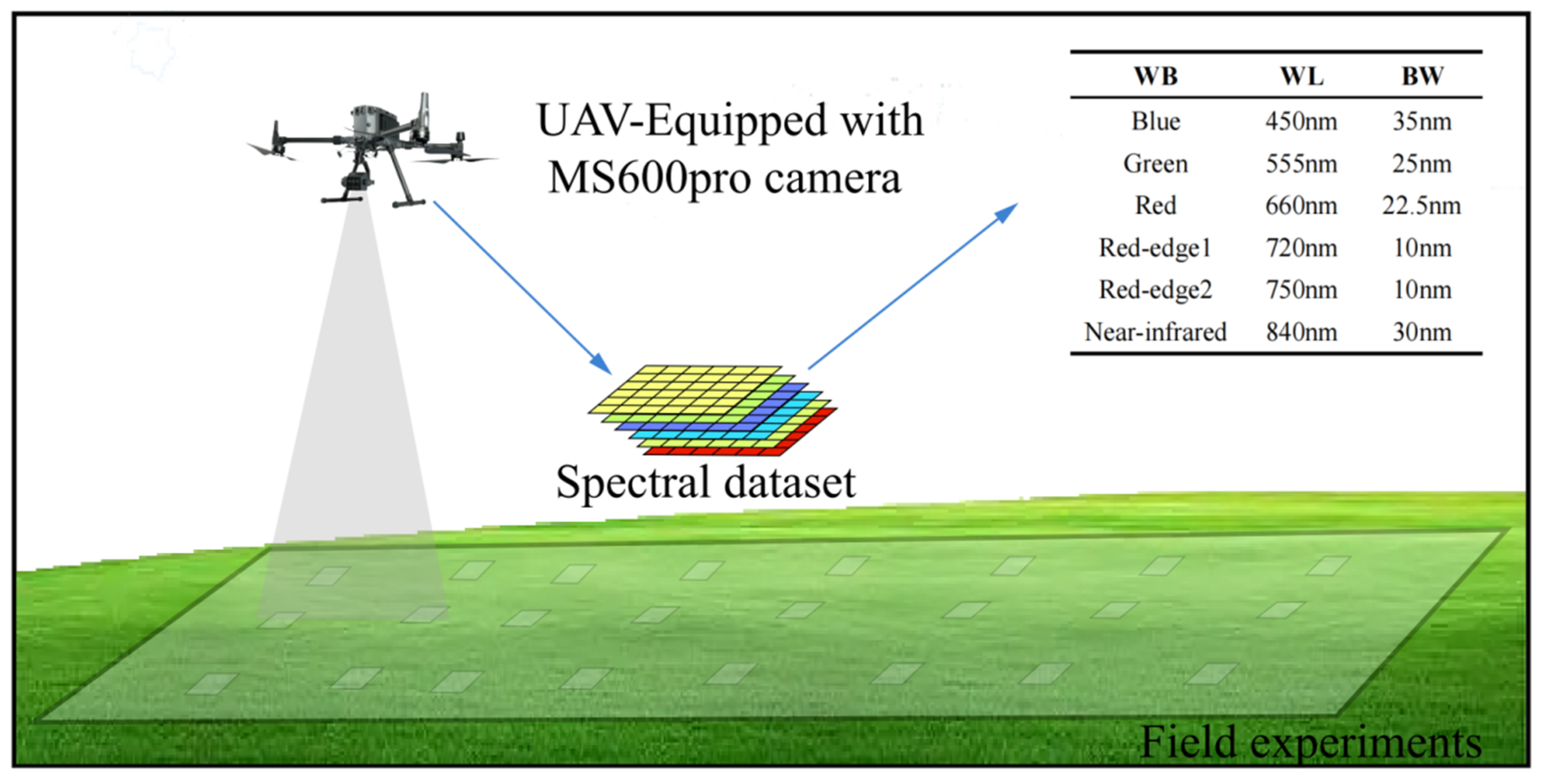
2.2. Unmanned Aerial Vehicle (UAV) Sensor Platform

The UAV system in the study comprised a Matrice 300 RTK drone (Da-Jiang innovation Science and Technology Company, Shenzhen, Guangdong, China) and MS600 Pro camera (Yusense Information Technology and Equipment Incorporated Company, Qingdao, Shandong, China) for spectral data collection (Figure 2). The Matrice 300 RTK drone is a quadrocopter equipped with a GPS and Inertial Measurement Unit (IMU), with a flight time of more than 35 min when equipped with the MS600 Pro camera. The MS600 Pro camera is a multi-spectral sensor and contains 6 spectral bands, including red, green, blue, red-edge1, near-infrared, and red-edge2 wavebands. In this study, the camera was used to collect spectral data within the cage at difference growth stages with various density levels of O. decorus.

2.3. Field Experiment

The field experiments were conducted from 18 June 2022 to 12 July 2022. O. decorus nymphs from second to fifth instar larvae were applied because first instar nymphs are too small to be captured. The processing of field experiments can be divided into three steps. Step 1: after selecting the study area, 24 cages were assembled and weeds except Leymus chinensis were removed from each plot. Step 2: more than one thousand O. decorus nymphs were captured and various numbers of nymphs were placed in each cage according to the density level (0, 8, 15, 22, 30, 45, 60, and 90 nymphs/m2), respectively. Then, the number was counted (twice a day) and nymphs were added to corresponding cages if any nymphs suffered death or escaped. Step 3: the growth stages of nymphs (Figure 3) were verified, and if more than eighty percent of the nymphs completed molting, the growth stages of the nymphs were considered to be changed. Then, all cages were removed and spectral data of all plot canopies were collected by the UAV system. A flight altitude of 30 m above the ground level was set. The camera provided an image size of 1280 × 960 pixels. More than one hundred and fifty multi-spectral images of the study area were collected by the UAV system at set intervals. After spectral images were collected, the cages were moved back, and step 2 and step 3 were repeated. Finally, spectral data of five periods were collected by the UAV system.
(1)
On 19 June 2022, multi-spectral images were collected by the UAV system as initial data. Then, all cages were installed and different numbers of O. decorus nymphs (0, 8, 15, 22, 30, 45, 60, and 90 nymphs/m2) were placed in corresponding cages (Figure 1C).
(2)
On 28 June 2022, eighty percent of second instar nymphs had transformed to third instar nymphs in most cages. All cages were removed and spectral images were collected using the UAV system. Subsequently, all cages were moved back to continue the experiments.
(3)
On 3 July 2022, more than eighty percent of third instar nymphs had transformed to fourth instar nymphs in most cages. All cages were removed. Spectral images of all plot canopies were taken by the UAV system.
(4)
On 8 July 2022, fourth instar nymphs in the cages had basically molted. Spectral images were collected after removing all cages.
(5)
On 11 July 2022, more than eighty percent of fifth instar nymphs had transformed to adults. However, spectral data could not be collected due to poor weather conditions until the field experiment was completed on the following day.

2.4. Multi-Spectral Image Processing

All multi-spectral images of UAV were processed in Yusense Map software (Version 2.2.3, http://mapupdate.yusense.com.cn:9092 (accessed on 13 March 2022)), including band registration, image mosaic, radiometric calibration, and vegetation indices calculation. Nine vegetation indices were derived from radiometric calibration-corrected reflectance to estimate vegetation loss caused by O. decorus at different growth stages and densities. Four commonly used vegetation indices in plant monitoring, the normalized difference vegetation index (NDVI), enhanced vegetation index (EVI), ratio vegetation index (RVI), and difference vegetation index (DVI), were derived from processing data in the red, near-infrared, and blue wavebands. Furthermore, the soil-adjusted vegetation index (SAVI) and modified soil-adjusted vegetation index (MSAVI) were derived from the red and near-infrared bands to reduce soil noise [29]. In order to investigate the change in leaf chlorophyll content after invasion by O. decorus, the green chlorophyll vegetation index (GCVI) and Red Edge Ratio Index (RRI) were estimated, which are sensitive to leaf chlorophyll content [30,31]. Ultimately, nine vegetation indices were calculated for each plot during five periods. All vegetation indices (VIs) and their formulas are displayed in Table 1.

2.5. Variation of Vegetation Indices
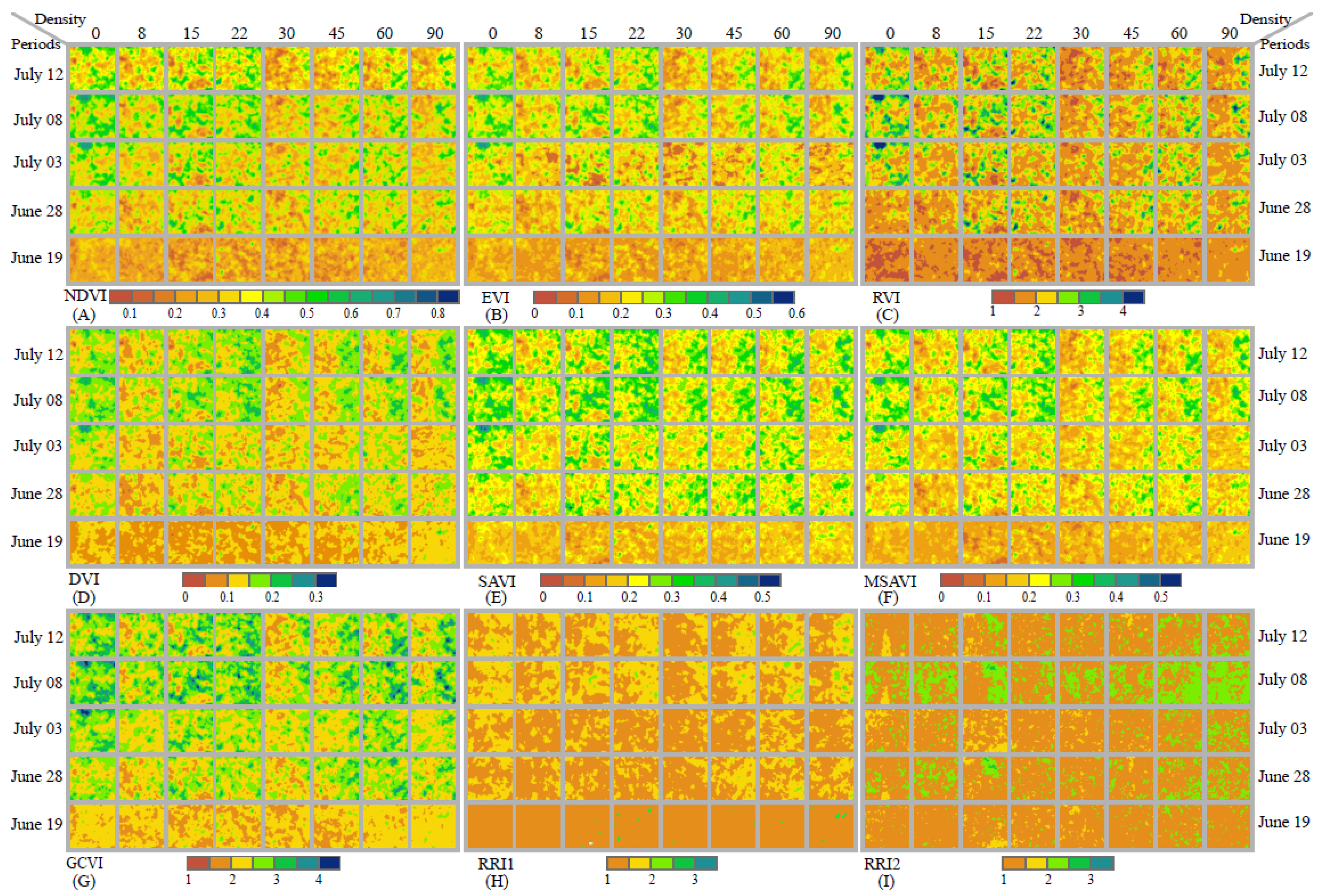
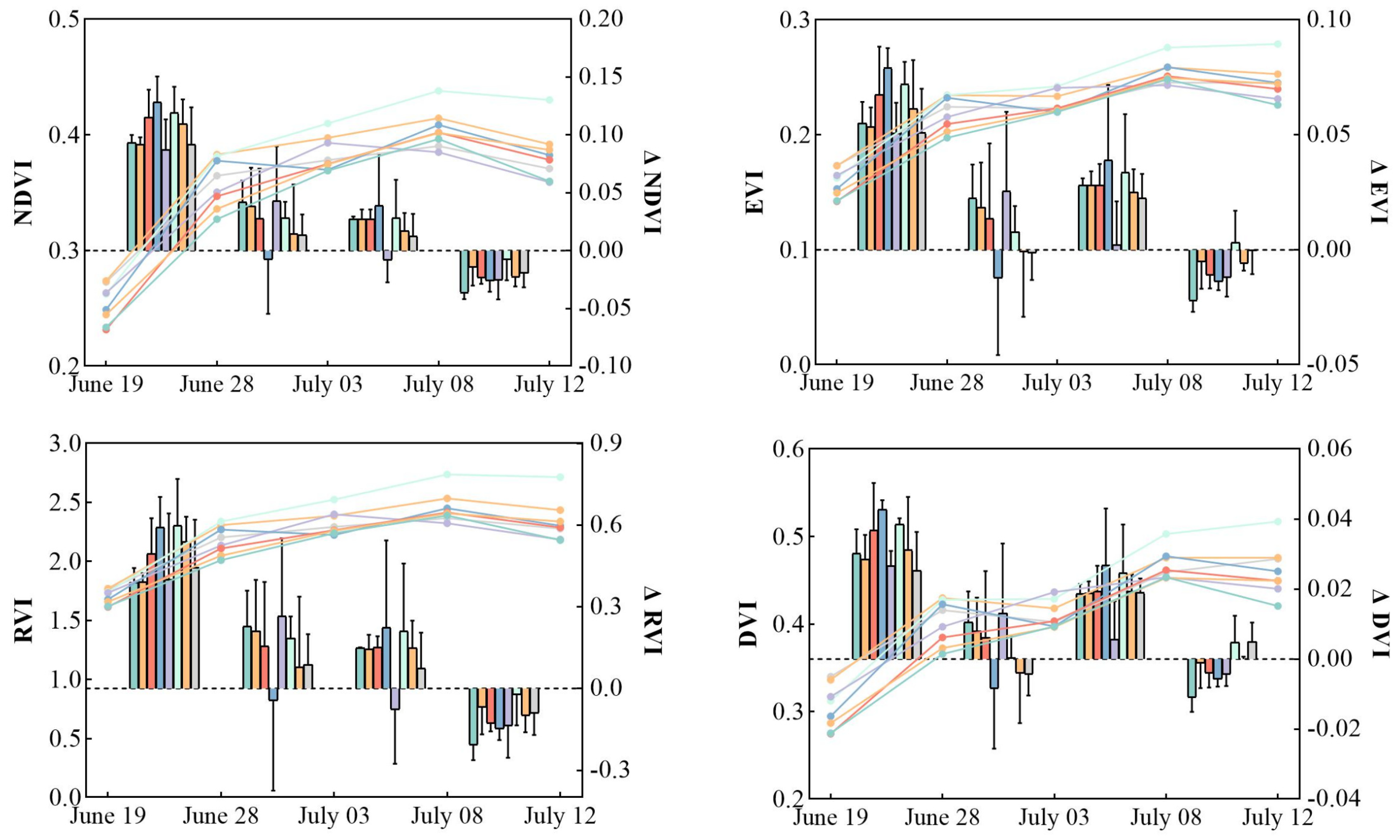
To improve the understanding of plant loss caused by O. decorus at different growth stages and different density levels, the variation of VIs and losses of VIs were calculated using Formulas (10) to (11):
Δ VIs ( i , d ) = VIs ( i , d ) VIs ( i 1 , d )
where ΔVIs(i,d) means the variation of VIs between VIs(i,d) and VIs(i−1,d). VIs(i,d) represents the vegetation indices at time i (i represents four periods, on 28 June, 4 July, 8 July, and 12 July) of density level d (d = 0, 8, 15, 22, 30, 45, 60, and 90 nymphs/m2). VIs(i−1,d) indicates the vegetation indices on 19 June, 28 June, 4 July, and 8 July.
LVIs ( i , d ) = Δ VIs ( i , d ) Δ VIs ( i , 0 )
where LVIs(i,d) means the loss component of VIs at time I; ΔVIs(i,d) means the variation of VIs at time i with density level d. ΔVIs(i,0) indicates the vegetation index at time i with a density of 0 nymphs/m2. ΔVIs(i,d) and ΔVIs(i,0) were calculated using Formula (10).

3. Results

3.1. Response of Plant Vegetation Indices to O. decorus Invasion

The spectral characteristics of plants in the visible and near-infrared bands are well known to vary after pest invasion. Many vegetation indices have been widely used to monitor and predict damage caused by insects. This study calculated nine vegetation indices to explore the most efficient indicator reflecting vegetation diversity in the five periods under different density levels of O. decorus. The results are presented in Figure 4.
The vegetation indices were found to reveal the characteristics of biomass change in each cage during the study periods. On June 19, multi-spectral images were collected using the UAV system as the initial data, and nine vegetation indices (Figure 4) were derived for cages that had little difference in plant status at that moment. However, some differences in the nine plant vegetation indices appeared under different density levels in the other four periods. For instance, the NDVI (Figure 4A) showed little difference in variation between the experiment group (the number of nymphs greater than 0) and the control group (the number of nymphs was 0) on 28 June. On 3 July, however, large variations began to emerge between the experiment and control groups. The NDVI of cages with O. decorus densities of <22 nymphs/m2 and ≥30 nymphs/m2 displayed significant differences. The NDVI increased during the study periods when the density level of O. decorus was less than 22 nymphs per cage (nymphs/m2). If the density was equal to or greater than 30 nymphs/m2, NDVI exhibited a slow increase or negative growth. On 8 July and 12 July, the distinction became even more pronounced. Overall, EVI, RVI, DVI, SAVI, and MSAVI (Figure 4B–F) presented similar change characteristics to NDVI. An interesting phenomenon was found in that all vegetation indices exhibited large differences between cages with density levels of <22 nymphs/m2 and ≥30 nymphs/m2. In addition, the VI of cages with density ≥ 15 nymphs/m2 was higher than that of cages with a density of 0 or 8 nymphs/m2.
The other three vegetation indices were computed to investigate the change in leaf chlorophyll content. The GCVI (Figure 4G) appeared to be more sensitive to leaf chlorophyll content compared with RRI 1 (Figure 4H) and RRI 2 (Figure 4I). On 28 June, the GCVI values of cages with density levels of 45, 60, and 90 nymphs/m2 were higher than those in other experimental groups (8, 15, 22, 30 nymphs/m2). RRI 1 exhibited a similar pattern. In contrast, RRI 2 was higher not only in cages with density levels of 45–90 nymphs/m2, but also in cages with density levels of 8 and 15 nymphs/m2. On 3 July, 8 July, and 12 July, GCVI or RRI 1 did not show clear differences between the experimental groups. Although little differences in RRI 2 were observed among the experimental cages on 3 July, large variations emerged in cages with density levels of 60 and 90 nymphs/m2 and in other cages on 8 July and 12 July.

3.2. Variation Characteristics of Vegetation Indices Attributable to O. decorus

To better explore and understand the variation characteristics of the nine vegetation indices attributable to the different density levels of O. decorus at different growth stages, and to select appropriate indices to represent the above-ground biomass of Leymus chinensis, the average vegetation index of each cage was calculated. The change trend of each vegetation index and the change value between two adjacent times were obtained. The variations were then plotted, as shown in Figure 5.
During the study period, the variation trend of NDVI showed a general increase. From 19 June to 28 June, the second instar nymphs of O. decorus transformed to third instar nymphs. The NDVI value of each cage increased significantly under different density levels, especially in cages with density levels of 15, 22, 45, and 60 nymphs/m2. From 28 June to 3 July, O. decorus transformed from third instar to fourth instar nymphs. The growth rate of the NDVI became slower than that in the last stage. In cages with a density level of 22 nymphs/m2, even negative growth was observed. The NDVI of cages with high density (60, 90 nymphs/m2) increased more slowly than that of cages with low density. A similar trend was observed in next period, during 3 July to 8 July (the transformation of O. decorus into fifth instar nymphs). From 8 July to 12 July, fifth instar nymphs transformed to adults. The NDVI values of all cages significantly decreased. The trend characteristics of other vegetation indices and the NDVI were generally consistent during the study periods. However, a large difference was observed in the EVI, DVI, SAVI, and MSAVI on 3 July to 8 July compared to the NDVI. The EVI, DVI, SAVI, and MSAVI increased further with reference to the last periods.
The other three vegetation indices were used to reveal and represent the chlorophyll content of plant leaves. Significant differences were observed in the trends of these vegetation indices (GCVI, RRI 1, and RRI 2). The GCVI gradually increased during the study period, although the rate of change gradually decreased. The period from 19 June to 28 June corresponds to the second instar nymphs of O. decorus. In cages with a density level of 45 nymphs/m2, the GCVI increased more rapidly than in other cages, followed by cages with densities of 60, 22, 15, 90, 0, 8, and 30 nymphs/m2. From 28 June to 3 July (third instar nymphs), most of the cages showed an increasing trend in GCVI, which was lower than before. Only cages with a density level of 30 nymphs/m2 showed negative growth. From 3 July to 8 July (fourth instar nymphs), the GCVI increased at a lower rate in cages with densities of 0, 8, and 30 nymphs/m2, while other cages showed higher increasing rates than in the third instar nymphal stage. From 8 July to 12 July (fifth instar nymphs transforming to adults), the GCVI showed a decreasing trend in most experimental cages.
Although RRI 1 and RRI 2 were derived from the red edge bands and red bands of UAV multi-spectral images, they both exhibited significant differences. The change trend of RRI 1 was more similar to that of the EVI. In the second instar nymphal stage (19 June to 28 June) of O. decorus, RRI 1 showed higher increases in all cages than in any other period. During the third instar nymphal stage (28 June to 8 July), RRI 1 in those cages showed a lower increase or a negative increase in cages with densities of 0, 8, 30 nymphs/m2, and 22, 45, 60, 90 nymphs/m2, respectively. The vegetative index of RRI 1 in each cage increased rapidly during the fourth instar nymphal stage. When grasshoppers transformed from fifth instar nymphs to adults (8 July to 12 July), RRI 2 decreased in the sample plots, except for cages with densities of 8, 15, and 45 nymphs/m2, which showed a slight increase. On the contrary, from 19 June to 28 June, the growth rate of RRI 2 was far below that of the other eight vegetation indices in cages with different densities. The growth rate of RRI 2 decreased with increasing grasshopper densities. In the third instar nymphal stage (28 June–8 July), the growth of RRI 2 was higher in all cages than in any periods. In the other two periods, RRI 2 showed a negative increase.

3.3. Relationship between the Loss Component of Leymus Chinensis and the Density Level of O. decorus

Formula (11) was used to estimate the loss components of Leymus chinensis attributable to O. decorus in four periods (second, third, fourth, and fifth instar nymphal stages). SPSS 20.0 was applied to deduce the relationship between grasshopper density and the nine VIs in the four growth stages. All equations are shown in Table 2. Regrettably, most VIs showed poor correlation with grasshopper density. During the second instar nymphal stage of O. decorus, the RVI presented the strongest relationship between vegetation loss and nymph density (R2 = 0.788). The RVI increased when the grasshopper density was less than 30 nymphs/m2, and decreased when the grasshopper density was greater than 30 nymphs/m2. However, the R2 of the other eight VIs with grasshopper density was mostly less than 0.4, or even less than 0.2. A similar phenomenon was observed in the third instar nymphal stage. Compared with other VIs, the RVI presented excellent performance in reflecting plant loss (R2 = 0.6113). When the grasshopper density was less than 45 nymphs/m2, plant loss gradually decreased. If grasshopper density in a cage was greater than 45 nymphs/m2, plant loss gradually increased. In contrast, the other VIs continued to show few good results for estimating the loss of vegetation at this time. With the increase of the density level of O. decorus, plant loss exhibited an increasing trend, according to the relationship between RVI variation and grasshopper density during the fourth instar nymphal stage. Other VIs could not reflect plant loss well in this period. In the next period, fifth instar nymphs transforming into adult grasshoppers, the DVI appeared to be the best indicator (R2 = 0.3165) of damages damage caused by the grasshopper.

4. Discussion

The Earth has seen several grasshopper plagues in recent years [6]. It is, thus, becoming increasingly essential to find means of reducing losses caused by such plagues. Specifically, the accurate monitoring and prediction of such incidents plays a vital role [32]. Therefore, understanding the underlying mechanisms of grasshoppers with different densities affecting plants is a fundamental task for grassland protection. Many studies have been conducted and their results have indicated that vegetation indices fully support the estimation of plant loss caused by grasshoppers at different densities [3,13,14]. However, previous studies focused on the simulation of plant loss under various densities of adult grasshoppers and different damage duration treatments. Only a few studies have explored damages caused by grasshoppers at different growth stages.
In this study, spectral data were acquired for multiple cages accounting for each growth stage using a UAV equipped with a multi-spectral camera. Nine VIs were derived from the acquired data to identify to the most suitable index for estimating plant loss caused by O. decorus during different growth stages. The results showed that there was no significant difference in VIs between the experimental and control groups in the second instar nymphal stage (from 19 June to 28 June) of O. decorus, until the third instar nymphal stage (from 28 June to 30 July), when VIs began to show some variation between cages with densities of <22 nymphs/m2 and ≥30 nymphs/m2. These results suggest that O. decorus caused little harm to plants in the second instar nymphal stage [18]. The decrease in VIs mainly started from the third instar nymphal stage, especially when the nymph density of O. decorus was ≥30 nymphs/m2.
To improve research on the underlying mechanisms between the variations of the nine VIs and the density of O. decorus during the four growth stages, the average VIs per cage were calculated. VIs were found to increase in many cages during the study period. With the change in the growth stage and density per unit of O. decorus, however, significant differences in the variation of VIs (ΔVIs) appeared (Figure 5). In the second instar nymphal stage, as the population density increased, ΔVIs increased and then declined in many cages. Moreover, ΔVIs increased more in this stage than in the other three growth stages. From the third to fifth instar nymphal stages, ΔVIs showed a downward trend, and even a negative trend in the fifth instar nymphs. These results reveal that second instar nymphs could promote plant growth [33]. However, as the nymphs increase in density and age, this phenomenon would slowly disappear.
In addition, the relationship between the loss components of plants and the density levels of nymphs at different instar nymphal stages was investigated. Compared with other VIs, the RVI appeared as the most excellent vegetation index for reflecting the relationship between plant loss and the unit density of O. decorus in the second, third, and fourth instar nymphal stages. According to the equation of nymph density and the RVI in the second instar nymphal stage, low nymph density (less than 60 nymphs/m2) would promote the growth of Leymus chinensis. With the increase in the number of nymphs, the biomass of each cage increased (nymph density < 30 nymphs/m2) and then decreased (nymph density ≥30 nymphs/m2). After the nymph density exceeded 60 nymphs/m2, the biomass showed negative growth. These results further confirmed that second instar nymphs with lower unit density could promote plant growth. However, in the third instar nymphs, it was surprising that plant loss components were significantly lower in cages with densities of 45 and 60 nymphs/m2 than those in other cages (nymph density < 45 nymphs/m2 or 90 nymphs/m2). This unexpected result requires further study. During the fourth and fifth instar nymphal stages of O. decorus, the loss components showed positive correlations with nymph density. Furthermore, the most serious damage by O. decorus was observed in the fourth instar nymphal stage. As the above-ground biomass of each cage was not collected in this study, the relationships between above-ground biomass and VIs or the density of O. decorus were not explored. Nevertheless, this study investigated and explored the underlying mechanisms between nine VIs and O. decorus density in each cage, and some results will guide the development of monitoring and control measures for reducing damages caused by O. decorus.

5. Conclusions

In this study, a UAV equipped with a multi-spectral camera was used to investigate the underlying mechanisms between plant loss and O. decorus density in individual cages at different growth stages. The results confirmed that multi-spectral data can reveal plant loss caused by grasshoppers. The ratio vegetation index (RVI) was found to be the most excellent index for reflecting Leymus chinensis loss caused by O. decorus at different growth stages. At low density, second instar nymphs of O. decorus can promote vegetation growth. However, as the growth stage progresses, this phenomenon slowly disappears. The biomass damage caused by nymphs mainly started from the third instar nymphal stage. Plant loss was greater in the fourth instar nymphal stage than in other stages. These results can guide the development of monitoring and prediction measures to decrease damage.

Author Contributions

B.D. and X.D. are co-first authors of the article. Conceptualization, B.D. and X.D.; methodology, B.D.; software, B.D.; validation, K.L., W.H. and N.W.; formal analysis, B.D.; investigation, X.D.; resources, N.W.; data curation, B.D., X.D. and C.J.; writing—original draft preparation, B.D.; writing—review and editing, N.W., Y.D. and W.H.; visualization, J.G. and L.L.; supervision, K.L.; project administration, N.W.; funding acquisition, N.W. All authors have read and agreed to the published version of the manuscript.

Funding

This research was funded by the Inner Mongolia Autonomous Region Science and Technology Planning Project, grant number 2021GG0069, the Central Public-interest Scientific Institution Basal Research Fund, grant number Y2021XK24, the Central Public-interest Scientific Institution Basal Research Fund, grant number 1610332023010, the National Key R & D Program of China (2022YFD1401102), SINO- EU, Dragon 5 proposal: Application Of Sino-Eu Optical Data Into Agronomic Models To Predict Crop Performance And To Monitor And Forecast Crop Pests And Diseases (ID 57457); additional funding by the Fengyun Application Pioneering Project (FY-APP).

Data Availability Statement

Not applicable.

Conflicts of Interest

The authors declare no conflict of interest.

References

  1. Kang, L.; Wei, L. Progress of acridology in China over the last 60 years. Acta Phytophylacica. Sin. 2022, 49, 4–16. [Google Scholar]
  2. Mariottini, Y.; Marinelli, C.; Cepeda, R.; DeWysiecki, M.L.; Lange, C.E. Relationship between pest grasshopper densities and climate variables in the southern Pampas of Argentina. Bull. Entomol. Res. 2022, 112, 613–625. [Google Scholar] [CrossRef]
  3. Song, P.L.; Zheng, X.M.; Li, Y.Y.; Zhang, K.Y.; Huang, J.F.; Li, H.M.; Zhang, H.J.; Liu, L.; Wei, C.W.; Mansararay, L.R.; et al. Estimating reed loss caused by Locusta migratoria manilensis using UAV-based hyperspectral data. Sci. Total Environ. 2020, 719, 137519. [Google Scholar] [CrossRef] [PubMed]
  4. Peng, W.X.; Ma, N.L.; Zhang, D.Q.; Zhou, Q.; Yue, X.C.; Khoo, S.C.; Yang, H.; Guan, R.R.; Chen, H.L.; Zhang, X.F.; et al. A review of historical and recent locust outbreaks: Links to global warming, food security and mitigation strategies. Environ. Res. 2020, 191, 110046. [Google Scholar] [CrossRef] [PubMed]
  5. Latchininsky, A.V. Locusts and remote sensing: A review. J. Appl. Remote Sens. 2013, 7, 075099. [Google Scholar] [CrossRef]
  6. Zhang, L.; Lecoq, M.; Latchininsky, A.; Hunter, D.; Douglas, A.E. Locust and Grasshopper Management. Annu. Rev. Entomol. 2019, 64, 15–34. [Google Scholar] [CrossRef]
  7. Chen, C.L.; Qian, J.; Chen, X.; Hu, Z.Y.; Sun, J.Y.; Wei, S.J.; Xu, K.B. Geographic Distribution of Desert Locusts in Africa, Asia and Europe Using Multiple Sources of Remote-Sensing Data. Remote Sens. 2020, 12, 3593. [Google Scholar] [CrossRef]
  8. Ni, S.; Wu, T. Monitoring the intensity of locust damage to vegetation using hyper-spectra data obtained at ground surface. In Proceedings of the Remote Sensing and Modeling of Ecosystems for Sustainability IV. SPIE, San Diego, CA, USA, 26–30 August 2007; Volume 6679, pp. 89–97. [Google Scholar]
  9. Moshou, D.; Bravo, C.; West, J.; Wahlen, S.; McCartney, A.; Ramon, H. Automatic detection of ‘yellow rust’ in wheat using reflectance measurements and neural networks. Comput. Electron. Agric. 2004, 44, 173–188. [Google Scholar] [CrossRef]
  10. Wu, T.; Ni, S.; Li, Y.; Zhou, X.; Chen, J. Monitoring of the damage intensity extent by oriental migratory locust using of hyper-spectra data measured at ground surface. J. Remote Sens.-Beijing 2007, 11, 103–188. [Google Scholar]
  11. Devesoni, E.D. Satellite normalized difference vegetation index data used in managing Australian plague locusts. J. Appl. Remote Sens. 2013, 7, 075096. [Google Scholar] [CrossRef]
  12. Shi, Y.; Huang, W.; Luo, J.; Huang, L.; Zhou, X. Detection and discrimination of pests and diseases in winter wheat based on spectral indices and kernel discriminant analysis. Comput. Electron. Agric. 2017, 141, 171–180. [Google Scholar] [CrossRef]
  13. Zhao, F.; Wang, Z.; Wang, H.; Wu, H.; Liu, H.; Wang, G.; Zhang, Z. The effects of hyper spectral change on grassland biomass after damage by Calliptamus abbreviates populations of different densities. Acta Prataculturae Sin. 2015, 24, 195–203. [Google Scholar]
  14. Zheng, X.; Song, P.; Li, Y.; Zhang, K.; Zhang, H.; Liu, L.; Huang, J. Monitoring Locusta migratoria manilensis damage using ground level hyperspectral data. In Proceedings of the 2019 8th International Conference on Agro-Geoinformatics, Istanbul, Turke, 16–19 July 2019; pp. 1–5. [Google Scholar]
  15. Lausch, A.; Heurich, M.; Gordalla, D.; Dobner, H.J.; Gwillym-Margianto, S.; Salbach, C. Forecasting potential bark beetle outbreaks based on spruce forest vitality using hyperspectral remote-sensing techniques at different scales. For. Ecol. Manag. 2013, 308, 76–89. [Google Scholar] [CrossRef]
  16. Du, B.B.; Wei, J.; Lin, K.; Lu, L.H.; Ding, X.L.; Ye, H.C.; Huang, W.J.; Wang, N. Spatial and Temporal Variability of Grassland Grasshopper Habitat Suitability and Its Main Influencing Factors. Remote Sens. 2022, 14, 3910. [Google Scholar] [CrossRef]
  17. Guo, J.; Lu, L.H.; Dong, Y.Y.; Huang, W.J.; Zhang, B.; Du, B.B.; Ding, C.; Ye, H.C.; Wang, K.; Huang, Y.R.; et al. Spatiotemporal Distribution and Main Influencing Factors of Grasshopper Potential Habitats in Two Steppe Types of Inner Mongolia, China. Remote Sens. 2023, 15, 886. [Google Scholar] [CrossRef]
  18. Zha, Y.; Gao, J.; Ni, S.; Shen, N. Temporal filtering of successive MODIS data in monitoring a locust outbreak. Int. J. Remote Sens. 2005, 26, 5665–5674. [Google Scholar] [CrossRef]
  19. Rong, J.; Xia, Z.; Baoyu, X.; Zhe, L.; Tuanji, L.; Chuang, L.; Dianmo, L. Use of MODIS data of detect the Oriental migratory locust plague: A case study in Nandagang, Hebei Province. Acta Entomol. Sin. 2003, 46, 713–719. [Google Scholar]
  20. Lehmann, J.R.K.; Nieberding, F.; Prinz, T.; Knoth, C. Analysis of Unmanned Aerial System-Based CIR Images in Forestry-A New Perspective to Monitor Pest Infestation Levels. Forests 2015, 6, 594–612. [Google Scholar] [CrossRef]
  21. Rango, A.; Laliberte, A.; Steele, C.; Herrick, J.E.; Bestelmeyer, B.; Schmugge, T.; Roanhorse, A.; Jenkins, V. Using Unmanned Aerial Vehicles for Rangelands: Current Applications and Future Potentials. Environ. Pract. 2006, 8, 159–168. [Google Scholar] [CrossRef]
  22. Xi, G.L.; Huang, X.J.; Bao, Y.H.; Bao, G.; Tong, S.Q.; Dashzebegd, G.; Nanzadd, T.; Dorjsurene, A.; Davaadorj, E.; Ariuaad, M. Hyperspectral Discrimination of Different Canopy Colors in Erannis Jacobsoni Djak-Infested Larch. Spectrosc. Spectr. Anal. 2020, 40, 2925–2931. [Google Scholar]
  23. Nasi, R.; Honkavaara, E.; Lyytikainen-Saarenmaa, P.; Blomqvist, M.; Litkey, P.; Hakala, T.; Viljanen, N.; Kantola, T.; Tanhuanpaa, T.; Holopainen, M. Using UAV-Based Photogrammetry and Hyperspectral Imaging for Mapping Bark Beetle Damage at Tree-Level. Remote Sens. 2015, 7, 15467–15493. [Google Scholar] [CrossRef]
  24. Tong, S.; Dong, Z.; Zhang, J.Q.; Bao, Y.B.; Guna, A.; Bao, Y.H. Spatiotemporal Variations of Land Use/Cover Changes in Inner Mongolia (China) during 1980–2015. Sustainability 2018, 10, 4730. [Google Scholar] [CrossRef]
  25. Wu, T.; Hao, S.; Kang, L. Effects of Soil Temperature and Moisture on the Development and Survival of Grasshopper Eggs in Inner Mongolian Grasslands. Front. Ecol. Evol. 2021, 9, 727911. [Google Scholar] [CrossRef]
  26. Du, G.L.; Zhao, H.L.; Tu, X.B.; Zhang, Z.H. Division of the inhabitable areas for Oedaleus decorus asiaticus in Inner Mongolia. Plant Prot. 2018, 44, 24–31. [Google Scholar]
  27. Lu, L.H.; Kong, W.Q.; Eerdengqimuge; Ye, H.C.; Sun, Z.X.; Wang, N.; Du, B.B.; Zhou, Y.T.; Wei, J. Detecting Key Factors of Grasshopper Occurrence in Typical Steppe and Meadow Steppe by Integrating Machine Learning Model and Remote Sensing Data. Insects 2022, 13, 894. [Google Scholar] [CrossRef]
  28. Zhou, X.R.; Chen, Y.; Guo, Y.H.; Pang, B.P. Population dynamics of Oedaleus asiaticus on desert grasslands in Inner Mongolia. Chin. J. Appl. Entomol. 2012, 49, 1598–1603. [Google Scholar]
  29. Liu, H.Q.; Huete, A. A feedback based modification of the NDVI to minimize canopy background and atmospheric noise. IEEE Trans. Geosci. Remote Sens. 1995, 33, 457–465. [Google Scholar] [CrossRef]
  30. Gitelson, A.A.; Kaufman, Y.J.; Merzlyak, M.N. Use of a green channel in remote sensing of global vegetation from EOS-MODIS. Remote Sens. Environ. 1996, 58, 289–298. [Google Scholar] [CrossRef]
  31. Gitelson, A.A.; Vina, A.; Ciganda, V.; Rundquist, D.C.; Arkebauer, T.J. Remote estimation of canopy chlorophyll content in crops. Geophys. Res. Lett. 2005, 32, 825. [Google Scholar] [CrossRef]
  32. Gomez, D.; Salvador, P.; Sanz, J.; Casanova, C.; Taratiel, D.; Casanova, J.L. Machine learning approach to locate desert locust breeding areas based on ESA CCI soil moisture. J. Appl. Remote Sens. 2018, 12, 036011. [Google Scholar] [CrossRef]
  33. Lu, H.; Yu, M.; Zhang, L.S.; Zhang, Z.H.; Long, R.J. Effects of foraging by different instars and densities of Oodles asiaticus Oedaleus asiaticus on forage yield. Plant Prot. 2005, 31, 55–58. [Google Scholar]
Figure 1. Location of the experimental site in the central and western part of Inner Mongolia, China (A). Picture of the plots for ground cage experiments taken by a UAV (B). The distribution of O. decorus density levels (C).
Remotesensing 15 04352 g001
Figure 2. Matrice 300 RTK drone equipped with MS600pro camera and major parameters of the camera; WB, WL, and BW represent wavebands, central wavelength, and bandwidth of multi-spectral images, respectively.
Remotesensing 15 04352 g002
Figure 3. Growth stages of O. decorus.
Remotesensing 15 04352 g003
Figure 4. Transformation of nine vegetation indices (NDVI, EVI, RVI, DVI, SAVI, MSAVI, GCVI, RRI 1, RRI 2) in each cage plot during five periods under different density levels of O. decorus. x−axis and y−axis indicate the density levels of O. decorus (grasshopper nymphs/m2), and five periods of instar larvae, respectively.
Remotesensing 15 04352 g004
Figure 5. Variation characteristics of each vegetation index during 5 periods and the difference between adjacent times. x−axis represents the time of collection of UAV images. Left y−axis and right y−axis indicate the average vegetation index of each sampling plot and difference in vegetation index between adjacent periods, respectively. The broken line chart presents average vegetation index, and histogram presents difference in vegetation index between adjacent periods.
Remotesensing 15 04352 g005aRemotesensing 15 04352 g005b
Table 1. Vegetation indices and calculation formulas.
Vegetation IndicesFormulaOrder
Normalized Difference Vegetation Index (NDVI) NDVI = ρ N I R     ρ R E D ρ N I R   +   ρ R E D (1)
Enhanced Vegetation Index (EVI) EVI = 2.5 × ρ N I R     ρ R E D ρ N I R   +   6.0 ρ R E D     7.5 ρ B L U E   +   1 (2)
Ratio Vegetation Index (RVI) RVI = ρ N I R ρ R E D (3)
Difference Vegetation Index (DVI) DVI = ρ N I R ρ R E D (4)
Soil-Adjusted Vegetation Index (SAVI) SAVI = ρ N I R     ρ R E D ρ N I R   +   ρ R E D + L × ( 1 + L ) (5)
Modified Soil-Adjusted Vegetation Index (MSAVI) MSAVI = 2 ρ N I R   +   1     ( 2 ρ N I R   +   1 ) 2     8 ( ρ N I R     ρ R E D ) 2 (6)
Green Chlorophyll Vegetation Index (GCVI) GCVI = ρ N I R ρ G R E E N 1 (7)
Red Edge Ratio Index (RRI 1) RRI 1 = ρ N I R / ρ E D G E 1 (8)
Red Edge Ratio Index (RRI 2) RRI 2 = ρ N I R / ρ E D G E 2 (9)
Note: ρNIR, ρRED, ρBLUE, ρGREEN, ρEDGE1, and ρEDGE2 represent the near-infrared, red, blue, green, red-edge1, and red−edge2 wavebands of MS600 pro sensor, respectively. L represents a soil–vegetation interaction term, with a value of 0.5.
Table 2. Relationship between the losses in VIs and density in the four growth stages of O. decorus.
Growth StagesSecond Instar LarvaeThird Instar LarvaeFourth Instar LarvaeFifth Instar Larvae
VIsEquationEquationEquationEquation
NDVIy = −7 × 10−6x2 + 0.0005x + 0.0077R2 = 0.2422y = −6 × 10−6x2 + 0.0005x − 0.0268R2 = 0.1085y = −0.0002x − 0.0011R2 = 0.3205y = −2 × 10−7 × 2 + 8E−05x + 0.0137R2 = 0.1143
EVIy = −7 × 10−6x2 + 0.0005x + 0.0012R2 = 0.3809y = 8 × 10−7x2 − 0.0003x − 0.0068R2 = 0.1302y = −6 × 10⁻⁵x − 0.0004R2 = 0.1048y = 0.0001x + 0.0109R2 = 0.1978
RVIy = −5 × 10−5x2 + 0.0033x + 0.0455R2 = 0.788y = −6 × 10−5x2 + 0.0074x − 0.2479R2 = 0.6113y = −0.0022x + 0.0659R2 = 0.6222y = −0.0002x + 0.0826R2 = 0.2205
DVIy = −4 × 10−6x2 + 0.0003x + 0.0005R2 = 0.2948y = 6 × 10−7x2 − 0.0002x − 0.0028R2 = 0.2522y = 5 × 10⁻⁶x + 0.0002R2 = 0.0001y = 0.0001x + 0.006R2 = 0.3165
SAVIy = −6 × 10−6x2 + 0.0005x + 0.0011R2 = 0.1832y = −0.0002x − 0.007R2 = 0.2342y = 1 × 10−6x2 − 0.0001x + 0.0015R2 = 0.1048y = 0.0001x + 0.0101R2 = 0.2855
MSAVIy = −−6 × 10−6x2 + 0.0005x + 0.0006R2 = 0.2834y = −0.0002x − 0.0065R2 = 0.1369y = −2 × 10⁻⁵x + 5E − 05R2 = 0.2011y = 0.0001x + 0.0099R2 = 0.3136
GCVIy = −6 × 10−5x2 + 0.0064x − 0.0381R2 = 0.4125y = 7 × 10−6x2 − 0.0019x − 0.0165R2 = 0.1313y = −3 × 10−5x2 + 0.0034x − 0.0358R2 = 0.2251y = 9 × 10−6x2 − 0.0012x + 0.0946R2 = 0.0174
RRI 1y = −3 × 10−5x2 + 0.0031x − 0.0311R2 = 0.352y = −0.0006x − 0.0146R2 = 0.2636y = −3 × 10−5x2 + 0.003x − 0.0276R2 = 0.3377y = 1 × 10−5x2 − 0.0012x + 0.0511R2 = 0.2464
RRI 2y = −7 × 10−5x2 + 0.0073x − 0.0182R2 = 0.1781y = −5 × 10−6x2 − 0.0003x − 0.0705R2 = 0.2087y = −7 × 10−6x2 + 0.0002x − 0.0139R2 = 0.1054y = −4 × 10−6x2 + 0.0008x + 0.0888R2 = 0.1115
Note: R2 represents the square of correlation between vegetation loss indices and O. decorus density during the four growth stages.
Disclaimer/Publisher’s Note: The statements, opinions and data contained in all publications are solely those of the individual author(s) and contributor(s) and not of MDPI and/or the editor(s). MDPI and/or the editor(s) disclaim responsibility for any injury to people or property resulting from any ideas, methods, instructions or products referred to in the content.

