Article

TCNet: A Transformer–CNN Hybrid Network for Marine Aquaculture Mapping from VHSR Images

1
College of Resources and Environment, Shanxi University of Finance and Economics, Taiyuan 030006, China
2
College of Environment and Resource Science, Shanxi University, Taiyuan 030006, China
*
Author to whom correspondence should be addressed.
Remote Sens. 2023, 15(18), 4406; https://doi.org/10.3390/rs15184406
Submission received: 26 July 2023 / Revised: 3 September 2023 / Accepted: 5 September 2023 / Published: 7 September 2023
(This article belongs to the Special Issue Advances in Deep Learning Approaches in Remote Sensing)

Abstract

:
Precise delineation of marine aquaculture areas is vital for the monitoring and protection of marine resources. However, due to the coexistence of diverse marine aquaculture areas and complex marine environments, it is still difficult to accurately delineate mariculture areas from very high spatial resolution (VHSR) images. To solve such a problem, we built a novel Transformer–CNN hybrid Network, named TCNet, which combined the advantages of CNN for modeling local features and Transformer for capturing long-range dependencies. Specifically, the proposed TCNet first employed a CNN-based encoder to extract high-dimensional feature maps from input images. Then, a hierarchical lightweight Transformer module was proposed to extract the global semantic information. Finally, it employed a coarser-to-finer strategy to progressively recover and refine the classification results. The results demonstrate the effectiveness of TCNet in accurately delineating different types of mariculture areas, with an IoU value of 90.9%. Compared with other state-of-the-art CNN or Transformer-based methods, TCNet showed significant improvement both visually and quantitatively. Our methods make a significant contribution to the development of precision agricultural in coastal regions.

1. Introduction

Marine aquaculture, which breeds, rears, and harvests aquatic plants or animals in the marine environment, is going through a period of rapid growth in recent years. The global production of mariculture has grown to 33.1 million tons in 2020, which is almost double than the production of 17.9 million tons in 2000 [1]. Obviously, it provides significant potential for the global seafood supply and economic development [2]. However, such rapid development can cause serious environmental concerns over marine water [3], sediment [4], and biodiversity [5]. Hence, it is important to ensure the accurate mapping of these mariculture areas for effective management and conservation of marine resources.
Remote-sensing technology is able to observe marine aquaculture areas in various spatial and temporal scales, which has the potential to overcome limitations of traditional field surveying methods [6]. To perform automatic extraction from remote-sensing images, previous researchers have developed various methods, which can be grouped into three categories: pixel-based methods [7,8], object-based image analysis (OBIA) [9,10,11,12], and CNN-based methods [13,14,15,16,17,18]. The pixel-based methods, which are generally developed based on medium spatial resolution images, rely on the spectrum or texture features analyses. OBIA is developed with the application of very high spatial resolution (VHSR) images [19], which generally performs better than the pixel-based methods. It first tries to segment the images into meaningful objects, and then classifies these image objects to identify the mariculture areas. Therefore, such methods can utilize more fruitful object-based features. Recently, the CNN-based methods, especially fully convolutional networks (FCNs) [20], have achieved great success in environmental remote-sensing fields [21,22]. In contrast to traditional handcrafted features, CNN models can effectively learn discriminative features and patterns by utilizing multi-layer learning [23,24]. Recent studies have further explored the classification ability of CNN models for multisource remote-sensing data [25,26,27,28].
However, there are several significant challenges for current CNN-based models to accurately extract mariculture areas from VHSR images. The first problem is identification of confusing marine objects in complex marine environments, which show high inter-class similarity and intra-class variance in VHSR images. For example, the marine aquaculture areas show totally different shapes, sizes, and colors when submerged in turbid water or strong waves, as indicated in Figure 1a,b. Meanwhile, parts of the marine aquaculture areas can also show different features with other parts (Figure 1c) but share similar structural patterns with impervious surfaces in the land area (Figure 1d). In such cases, semantic information at a global scale is important for improving the classification performance. However, within CNN models, the convolution operations are designed to extract local patterns instead of the required global representations. To address this issue, researchers have introduced a series of approaches to capture multi-scale information by enlarging the receptive fields. One direct way is to change the convolution operation. Such methods include using larger kernel size [29], atrous convolution [30], and pyramids based on images or features [31]. However, as more convolution operations may be applied to the padded areas, convolution with a larger kernel size or atrous rate makes the acquired features less effective. Another way is to integrate the attention mechanism into the module. The attention module is designed to capture global information from all pixels [32], which alleviates the above problems [33]. However, such methods normally consume significant memory and more computing costs for acquiring global context, making such methods less effective.
Meanwhile, the sequential down-sampling operations in CNNs, which lead to much smaller final feature maps compared to the original image, can also decrease the classification performance. As a result, such features generally produce coarser predictions and lower classification accuracies, especially when dealing with marine objects that exhibit detailed structures in HSR images. To address this issue, researchers have tried to recover the intricate spatial details by incorporating fine-resolution features in shallow layers. These approaches include multi-scale feature fusion [34,35,36], deconvolution [37], or up-pooling with pooling indices [38]. However, most existing methods simply stack these multi-level feature maps without considering potential noise in the shallow layers.
In conclusion, although the CNN-based methods have achieved great success in various classification tasks, it is still difficult to accurately delineate marine aquaculture areas from VHSR images. First, the CNN-based methods are less effective in acquiring global semantic information, which is difficult to identify various marine aquaculture areas in complex marine environments. Second, due to the down-sampling operations in CNNs, most of the current strategies are difficult to fully utilize the feature maps from the shallow layers to recover the lost information, which makes it difficult to accurately declinate the detailed structures of marine aquaculture areas in VHSR images.
To solve previously mentioned issues, it is beneficial to combine the advantages of CNN for modeling local details and fine-grained features and attention mechanism for capturing global context and long-range dependencies. Following this idea, we proposed a novel semantic segmentation model named Transformer–CNN hybrid Network (TCNet) for a more comprehensive understanding of the remote sensing data, enabling the accurate identification and mapping of mariculture areas in a complex marine environment. The main contributions of our study are summarized as follows.
(1)
This study presented a Transformer–CNN hybrid Network (TCNet) for the mapping of marine aquaculture from VHSR images;
(2)
A hierarchical lightweight Transformer module was proposed to capture long-range dependencies, which helped to identify various marine aquaculture areas in complex marine environments;
(3)
An attention-mechanism-based structure was employed to refine the feature space in long-span connections, which helped to decline detailed structures of the marine aquaculture areas.

2. Study Area

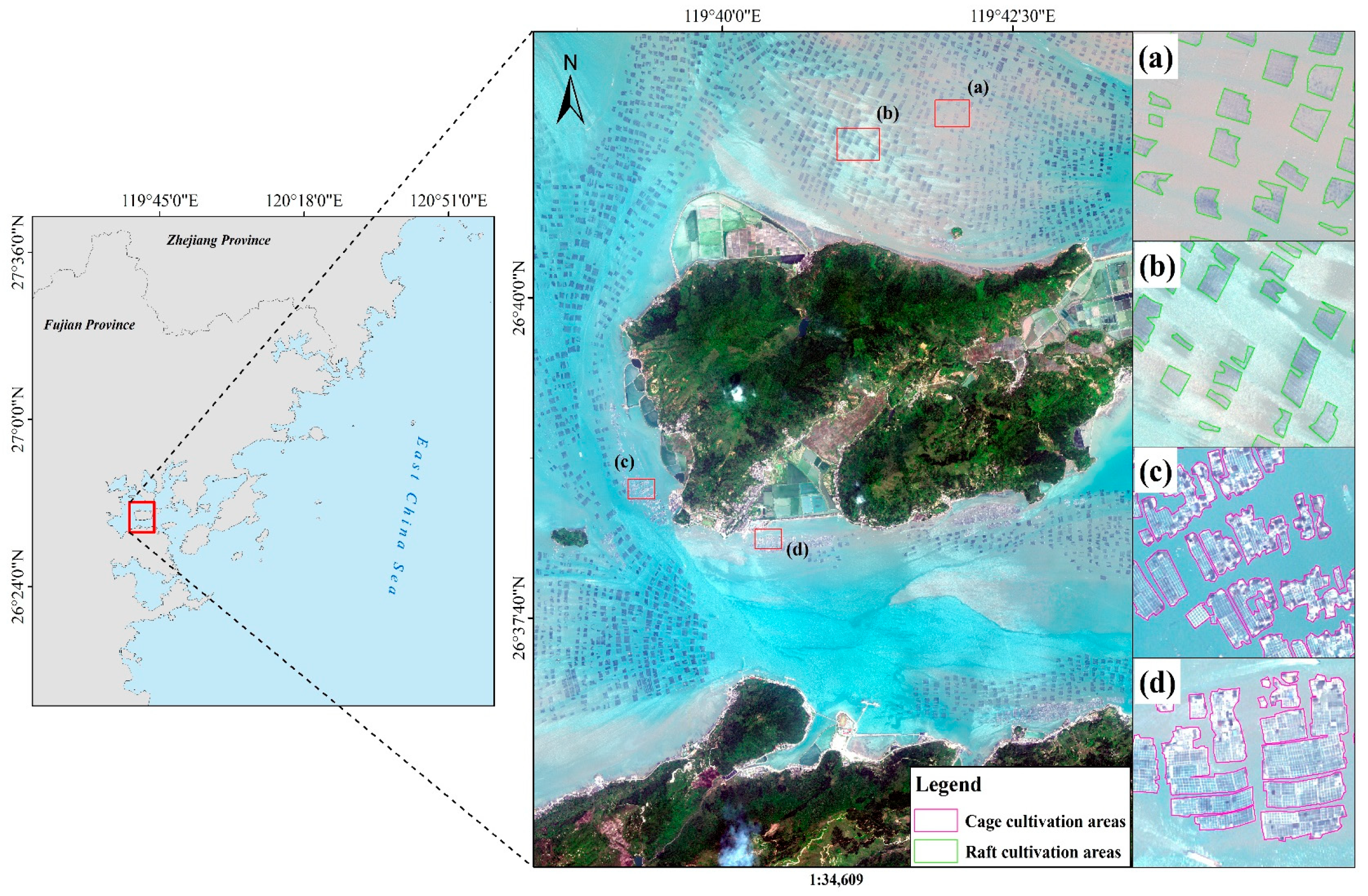
As shown in Figure 2, we selected a typical marine ranching area in Ningde City as our study area. As a coastal city located in the northeast of Fujian Province, China, Ningde City has a long coastline of 1046 km and abundant marine resources, which has become an important sector of the local economy. The marine aquaculture industry in Ningde has developed rapidly and formed extensive marine aquaculture areas, which mainly include raft culture area (RCA) and cage culture area (CCA).
The RCA is a type of aquaculture area that grows various aquatic plants, such as seaweed and agar, on floating rafts that are anchored in marine waters. In raft culture, aquatic organisms are grown on floating structures made of various materials, such as bamboo, wood, or plastic, so that they can float near the sea surface. The rafts are anchored to the seafloor or buoys and can be moved from one location to another as needed. As can be seen from Figure 2a,b, the RCA can vary in size or spectrum, depending on the number of rafts and the marine environment, such as the influence of turbid water or waves.
The CCA is another type of aquaculture area that grows various aquatic animals, such as fish and shellfish, in cages that are submerged in marine waters. In cage culture, the aquatic organisms are grown in cages made of various materials, such as netting or wire mesh, that allow water to flow freely through them. The cages are typically anchored to the seafloor. As can be seen from Figure 2c,d, the CCA can vary in size or texture, depending on the structure of rafts and the marine environment, such as the influence of light and the type of aquatic organisms being grown.

3. Materials and Methods

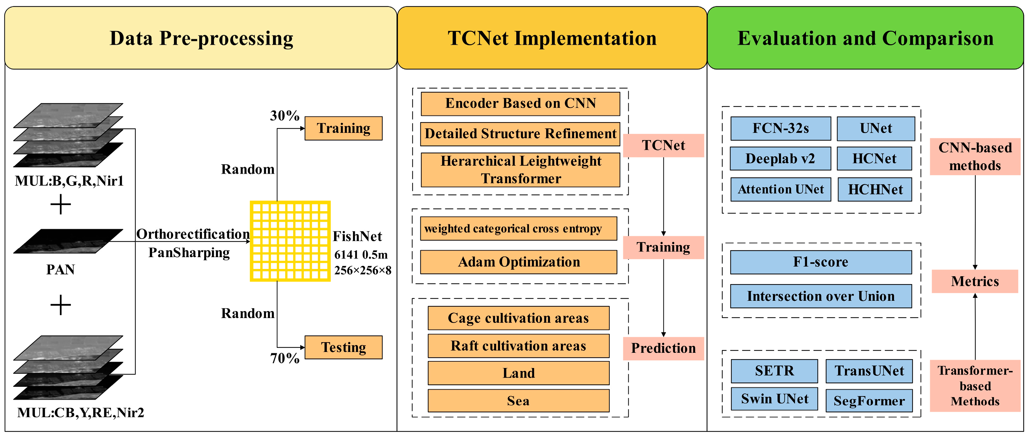
As shown in Figure 3, our methodological workflow can be divided into three parts, including data pre-process, TCNet implementation, and evaluation and comparison. The data pre-process was used to produce the training and testing datasets from VHSR images. And then, the TCNet was constructed with three important structures to extract different types of marine aquaculture areas from these datasets. Finally, we evaluated and compared the proposed methods with several state-of-the-art models.

3.1. Data and Preprocessing

In this study, the WorldView-2 (WV2) imagery was selected as our data source. Among VHSR (Very High Spatial Resolution) satellites like IKNOS, QuickBirds, GF-2, and SuperView-1, the WV2 (WorldView-2) sensor was selected for its superior characteristics. WV2 offers a higher spatial resolution of 2 m for multi-spectral bands, allowing for finer details to be captured. In addition to the standard blue, green, red, near-infrared, and panchromatic bands, WV2 provides several additional bands that contribute to its comprehensive spectral coverage. These additional bands include the coastal blue (400–450 nm), yellow (585–625 nm), red-edge (705–745 nm), and second near-infrared (860–1040 nm) bands.
The selected WV2 imagery was acquired on 20 May 2011 over the study area from DigitalGlobe (http://evwhs.digitalglobe.com, accessed on 1 September 2023). The satellite data were delivered at the product level of L2A, meaning that the values are presented as radiometrically corrected image pixels [39]. As the acquired images of the mariculture area exhibited excellent conditions without the presence of clouds, it was not necessary to perform atmospheric correction [40]. To process the acquired multi-spectral and panchromatic bands, we employed a three-step approach. Firstly, we orthorectified all the bands into the Universal Transverse Mercator (UTM) projection system. Orthorectification corrects the geometric distortions caused by terrain relief and sensor characteristics, ensuring accurate spatial alignment of the bands. After orthorectification, we performed a fusion of the multi-spectral and panchromatic bands using the Gram–Schmidt pan-sharpening module embedded in ENVI software (v5.3.1). This fusion process enhances the spatial details of the multi-spectral bands, resulting in a higher resolution and visually pleasing composite image. To improve the convergence rate of the network and reduce overfitting, the image pixels’ intensity values were normalized to the range of [0,1] using the liner stretch method.
Then, we first cropped the pre-processed image (see Figure 3) to more than 6000 non-overlapping patches with a size of 256 × 256 × 8. All these patches had a spatial resolution of 0.5 m. Among them, we randomly selected 70% of them to construct the training dataset. The other 30% areas of the images were used for testing dataset. Each of the patches was carefully labeled by visual interpretation (results can be found at https://github.com/yyong-fu/TCNet, accessed on 1 September 2023).

3.2. Transformer–CNN Hybrid Network

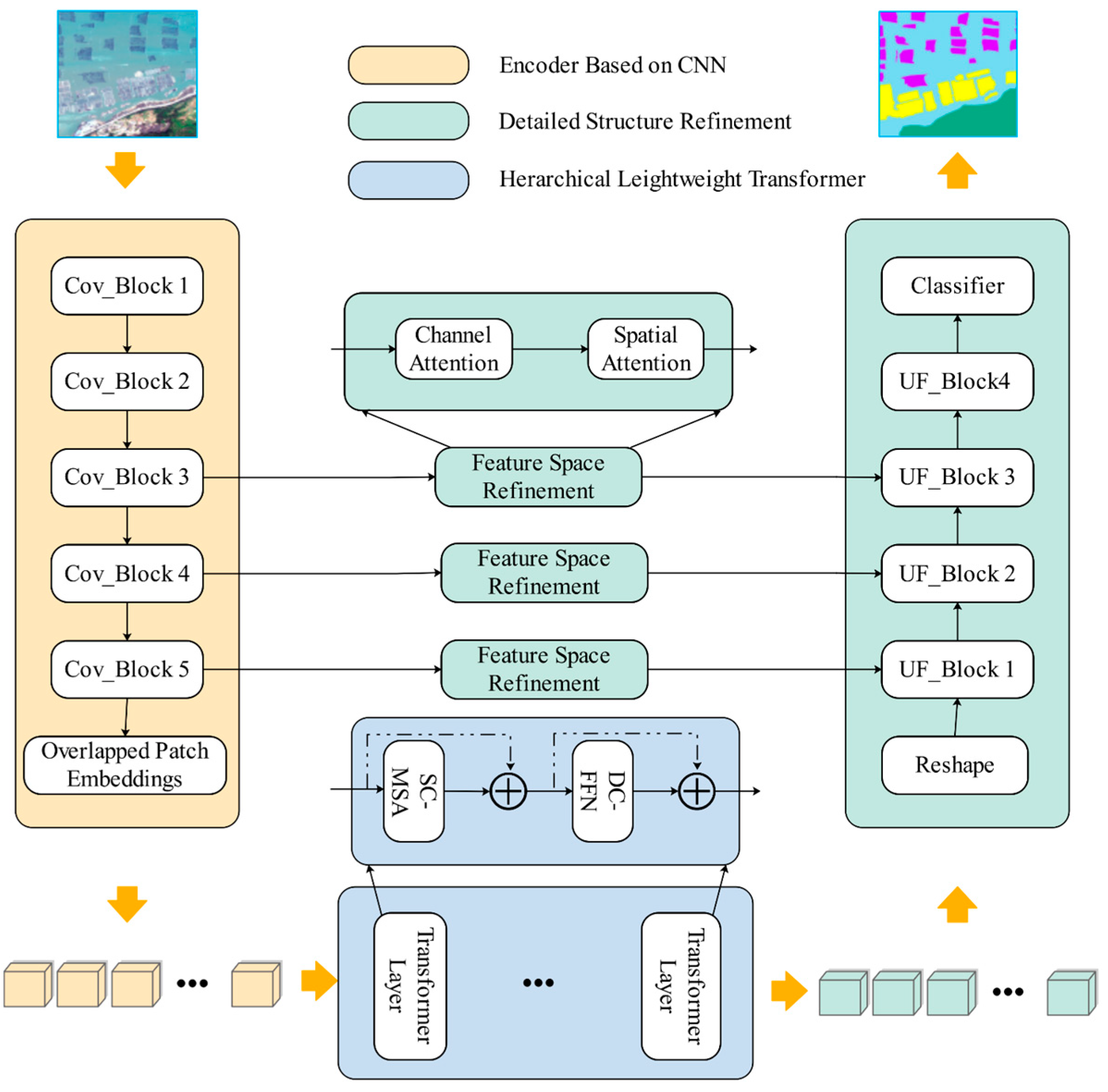
As shown in Figure 4, our proposed TCNet mainly included three parts. Specially, the TCNet first used a CNN-based encoder to extract high-dimensional feature maps from input images. After that, a hierarchical lightweight Transformer module was followed to capture the long-distance dependence among pixels of feature maps at global scale. We then used a coarse-to-fine strategy to gradually recover the detailed structure of marine aquaculture areas. In the following parts of this section, we will present the three major parts: (1) encoder based on CNN; (2) hierarchical lightweight Transformer; (3) detailed structure refinement.

3.2.1. Encoder Based on CNN

As shown in Figure 4, we first employed a CNN-based encoder to extract high-dimensional feature maps from images. To achieve the aim in an effective way, we employed the commonly used VGG-16 [41] as our encoder. VGG-16 is a lightweight CNN architecture with 16 layers. It consists of five blocks of convolutional layers, each followed by max-pooling layers. The first two convolutional blocks have two 3 × 3 convolutional layers with 64 filters and a max-pooling layer. The next two blocks have two 3 × 3 convolutional layers with 128 filters and a max-pooling layer. The fifth block has four 3 × 3 convolutional layers with 512 filters and a max-pooling layer. The network ends with three fully connected layers that perform the classification task. To obtain the original spatial information, we followed similar research [37,38] and removed all the fully connected layers. As the spatial resolution was vital for the following Transformer module, we removed the last two max pooling layers, and used the atrous convolutional layer with a dilation rate of 2 to enlarge the reception field. As a result, the spatial resolution of feature maps from the adopted VGG-16 based encoder was 1/8 of the input images, which was four times larger than the original feature maps.

3.2.2. Hierarchical Lightweight Transformer Module

Marine aquaculture areas showed more complicated human-made structures in VHSR images, making it difficult to achieve accurate segmentation without global semantic information. To capture such global information, traditional methods mainly focus on using an attention block at the end part of the architecture [32] or using the Transformer as encoder [42]. The former lost detailed information and the other one significantly increased the size of module and lost spatial information.
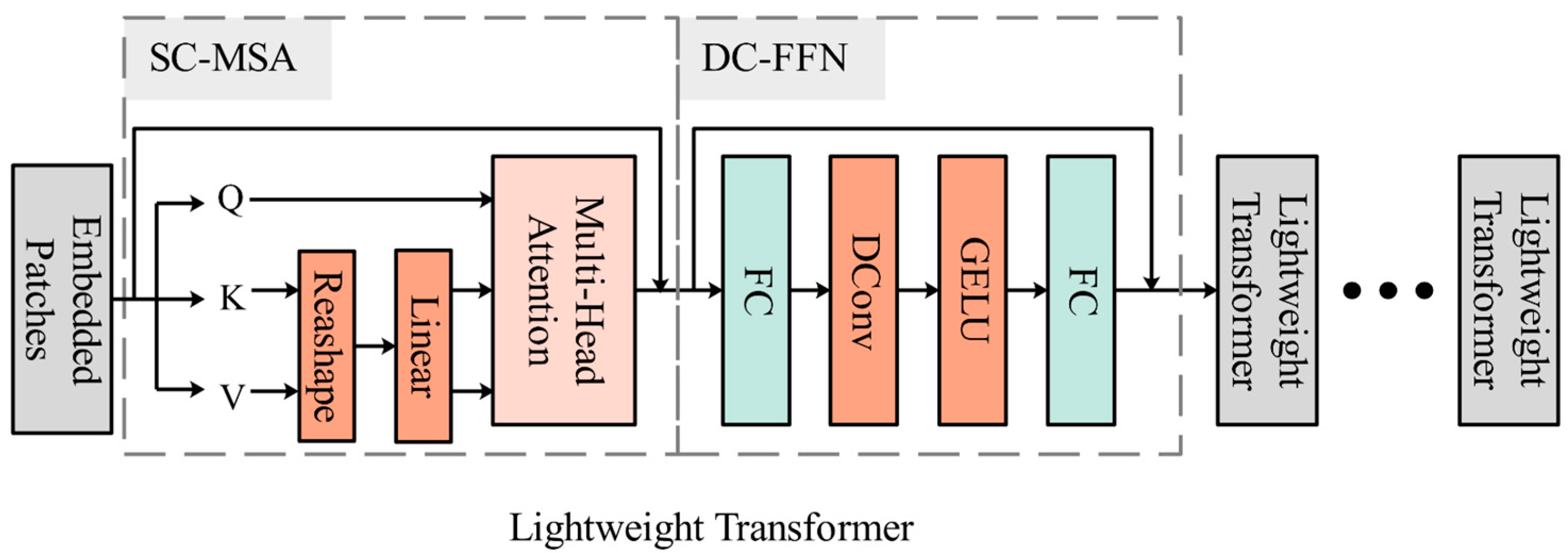
In contrast, we proposed to combine the spatial condensed Multi-Head Attention (SC-MSA) and the depth-wise convolution feed-forward network (DC-FFN) to build a lightweight Transformer module (see Figure 5). By arranging the proposed lightweight Transformer module in a hierarchical way, we were able to extract the global semantic information while maintaining high efficiency. Specifically, we first divided the feature maps to a serious of fixed-sized patches. Each patch’s pixel vectors were then flattened and fed into the lightweight Transformer layers. Finally, the transformer architecture was employed to learn global scale features by using the effective self-attention mechanisms, which allowed it to establish long-range dependencies between input patches. This means that the transformer can learn relationships between patches that are far apart in the input feature maps, allowing it to capture global information.
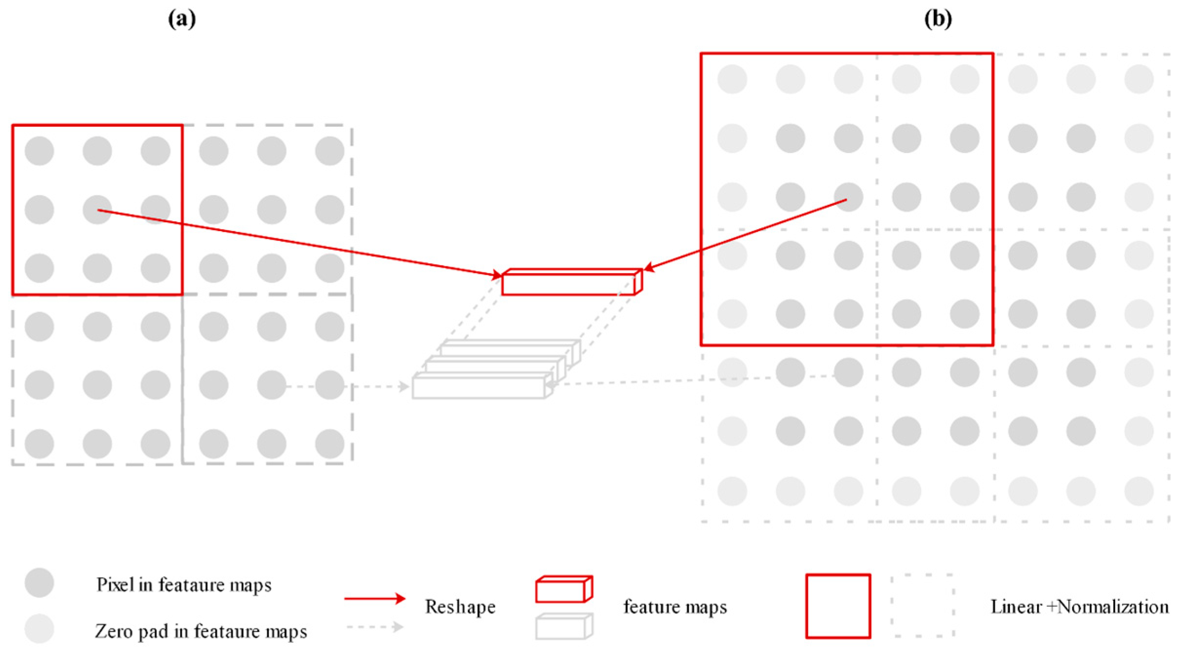
In the first stage, we employed the overlapping patch embedding to tokenize feature maps from the encoder, which can effectively capture and exchange local information [43]. As shown in Figure 6, we used the convolution operation with zero paddings to perform such operations. Specifically, giving the input feature maps with a size of H × W × C, we padded the feature maps with zeros to keep the resolution, and used a convolution with a kernel size of K × K, a stride size of S to perform the linear projection and obtain the embedded patches.
Second, the embedded patches were fed into the lightweight Transformer layers. As shown in Figure 5, each of these layers is composed of the SC-MSA and a DC-FFN. For the original Transformer layer [33], which is calculated as:
Attention   Q ,   K ,   V =   Softmax Q K T d K V ,
where Q, K, and V is the input sequence of query, key, and value in each one of the head, respectively. And dK is the dimension of sequence K.
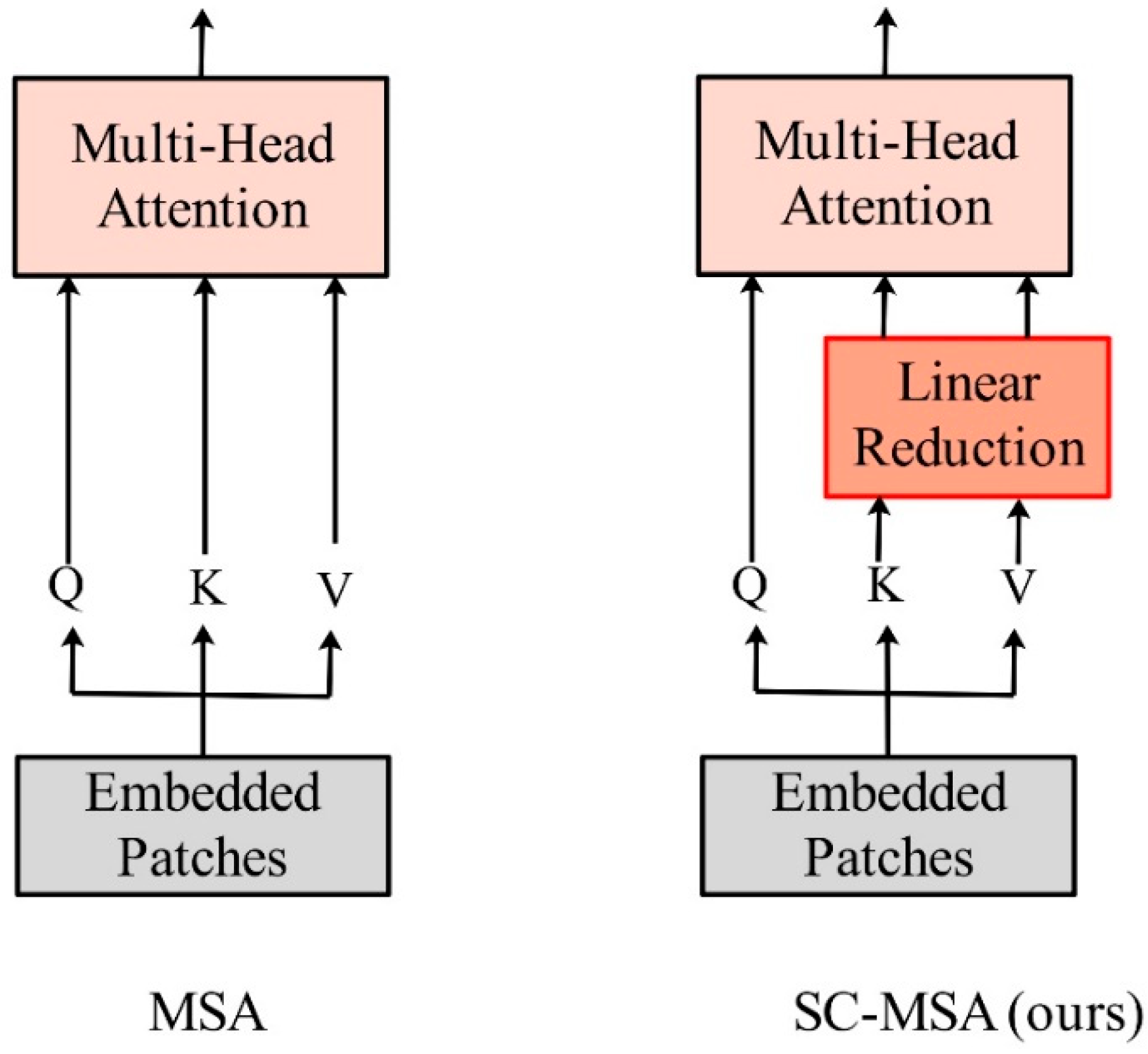
As existing of high-resolution features maps from the encoder, it significantly increases computation cost for the original MSA operation. To alleviate such problem, a reduction process was added to reduce length of the sequence as follows:
K n e w = Linear ( Reshape K o l d , N R , C · R , C ) ,
V n e w = Linear ( Reshape V o l d , N R , C · R , C ) ,
where Knew and Vnew is the compressed sequence, respectively. And Kold and Vold is the sequence to be compressed. The Reshape K o l d , N R , C · R , C means the operation that reshapes Kold to features with a shape of N R , C · R , where R is the reduction rate. The Linear (F, C) means the linear operation that projects feature F to feature maps with a shape of dimension C.
In the third stage, the original transformer generally uses fixed-size position encoding [44], which limits its generalization for longer input sequences once trained. Inspired by recent research [45,46], we removed the fixed-size position encoding. As shown in Figure 5, we employed the DC-FFN to achieve position encoding [43], which introduces the 3 × 3 depth-wise convolution with zero paddings in the middle part of FFN. The DC-FFN can be formulated as:
Fout = FC(GELU(DConv(FC(Fin)))) + Fin
where Fin represents the features from the SC-MSA. FC represents the fully connected layer. DConv represents the depth-wise convolution layer. GELU represents the GELU activation function [47].

3.2.3. Detailed Structure Refinement

Apart from identifying mariculture area in complex marine environments, mapping of the detailed structure presented in VHSR images is also a significant challenge. Actually, output feature maps from the encoder are much smaller than the original images, making it difficult for the recovery of lost information. To overcome this limitation, researchers have proposed various strategies to utilize the finer feature maps from shallow layers [34,48]. Following such idea, we proposed to refine the detailed structure of marine aquaculture areas with a coarser-to-finer strategy using long-span connections [13].
As shown in Figure 4, we performed such a strategy with several up and fuse blocks (UF block) in the decoder. Specially, we first concatenated the up-sampled features in the decoder and corresponding features from the encoder using long span connections. Then, we used a convolution layer with a kernel size of 3 × 3 to fuse the concatenated features. The whole process can be formulated as:
F d = Conv δ F i e © γ F i ,
where F d and F i are the output and input features of the UF block in decoder, respectively. F i e are the corresponding features of F i in the encoder. δ represents the feature space refinement process. γ represents the up-sampling process, which is a bilinear interpolation operation in our study. ‘ © ’ represents the concatenation process. Conv represents the convolutional process.
Meanwhile, as features from the encoder generally contain much noise information, direct concatenation of these features may not be the best way. Thus, we introduced an attention mechanism to refine the feature space, which is supposed to suppress noise and focus on the most useful channel and spatial part of the features [49]. The attention mechanism works by assigning weights or importance scores to different channels or spatial locations within the feature maps. To acquire such channel or spatial attention map, we first employed a global average pooling operation to generate a global context map on or along the channel axis. And then, the context map was fed into a multi-layer perceptron (MLP) to generate the attention map. The process can be formulated as:
F c s = F e F c a F s a ,
F c a = φ MLP C _ AvgPool F e , R ,
F s a = φ MLP S _ AvgPool F e , R ,
where F c s and F e represent the refined features and input features, respectively. F c a and F s a represents the channel and spatial attention map, respectively. C _ AvgPool ( ) and the S _ AvgPool ( ) represents global average pooling operation on or along the channel axis, respectively. MLP (F, R) represents the MLP containing a hidden layer with a reduction rate of R, which is set as 16 in our study. φ represents the sigmoid function.

3.3. Experimental Details

As shown in Figure 4, we first used a variant version of VGG-16 as the encoder to extract the high-dimensional and abstract features. Based on the extracted features, we employed a convolutional layer with 64 kernels with a size of 3 × 3 and a stride of 1 to obtain the embedded patches. After that, we used 8 Transformer layers to extract the semantic information, with the head number of 1, 1, 2, 2, 5, 5, 8, 8 and the reduction rate of 8, 8, 4, 4, 2, 2, 1, 1 in each layer. In the stage of detailed structure refinement, we used the output features from the last three convolutional blocks for refinement. Due to the application of atrous convolution layers, we skipped over the up-sampling processing in the last two UF blocks.
Following each one of the long span connections, we used a convolution layer with a kernel size of 1 × 1 to fuse concatenated features to a specific number, which is consistent with the corresponding kernel number in the encoder (i.e., 512, 512, 256). Finally, feature maps from the last up-sampling block were further up-sampled four times and produced the final results by using the softmax function, where a weighted categorical cross entropy with a weight of 1, 1, 2, 4 (corresponding to land, sea, RCA, CCA, respectively) was employed.
For the training of TCNet, we randomly selected 70% of regions from the pre-processed images, which were cropped to more than 6000 non-overlapping patches with a size of 256 × 256. Each of the patches was carefully labeled by visual interpretation. The other 30% areas of the images were used for accuracy assessment.
To conduct the experiments, we implemented the TCNet using Python version 3.6.0 programming language. We utilized the Keras library, specifically version 2.4.3, as the framework for developing the TCNet model. As the backbone of our implementation, we utilized Tensorflow version 2.6.0. During the training stage, we trained the TCNet for 30 epochs with a batch size of 32, and optimized by using Adam with a learning rate of 0.0001. The number of epochs are selected based on the training loss and curves (see Figure S1). And then, we performed the experiments based on a desktop workstation with one NVIDIA GTX 3090 GPU. Finally, the overall accuracy and training loss curves were recorded and are provided in Figure S1 in the Supplementary Material.

3.4. Comparison Methods

3.4.1. FCN-Based Methods

To evaluate the performance of our proposed TCNet, we first conducted a comparison with several state-of-the-art FCN-based methods. The main information of these models is summarized as follows.
FCN-32s: FCN-32s [20] is the first FCN-based model proposed for semantic segmentation of natural images, which replaces the fully connected layers of VGG-16 with convolutional layers to enable end-to-end learning. The model consists of three components: an encoder network, a decoder network, and a pixel-wise classifier. The encoder network is a VGG-16 model, and the decoder network converts the coarse feature maps from the encoder to fine maps. The pixel-wise classifier is a convolutional layer with the same size as the input image. It was selected as a baseline for all the FCN-based models in this study.
DeepLabv2: DeepLabv2 [30] is a semantic segmentation model that uses atrous convolution to expand the field of view of filters. It consists of a ResNet-101 model as the encoder, an atrous spatial pyramid pooling module, and a decoder network. As the typical method of acquiring multi-scale contextual information, which employs filters with different dilation rates in the atrous spatial pyramid pooling module, it is also suitable for comparison with the contextual information acquired by the Transformer-based module in TCNet.
U-Net: U-Net [34] is a typical encoder–decoder model for biomedical image segmentation. The encoder consists of a series of convolutional and max pooling layers, and the decoder consists of a series of up-sampling and convolutional layers. As the introduction of skip connections between the encoder and decoder, which concatenates feature maps from the encoder to the corresponding decoder layer to preserve fine-grained information, it was selected for comparison.
Attention U-Net: Attention U-Net [50] is an attention-based variant of the popular U-Net model. It introduces attention gates to selectively emphasize important features in the encoder and decoder networks. This improves the accuracy of segmentation, particularly in regions with complex boundaries or fine structures. Considering the similar encoder-decoder and attention gate in the Attention U-Net, it is also an ideal model for comparison.
HCNet: HCNet [13] is a hierarchical cascade neural network that is designed for mapping marine aquaculture areas using VHSR imagery. The main innovation of HCNet is the use of a cascade structure, which allows the model to learn features at different scales and resolutions. The model first extracts feature maps at a coarse scale, and then refines them at a finer scale in subsequent layers. This approach enables the model to accurately capture the complex spatial patterns and textures of marine aquaculture areas. HCNet outperforms several other state-of-the-art deep learning models in terms of mapping accuracy, demonstrating its effectiveness for fine-resolution mapping of marine aquaculture areas.
HCHNet: HCHNet [14] is a variant version of HCNet for mapping mariculture areas from medium spatial resolution, which includes two cascaded stages of convolutional neural networks. The first stage is a high-resolution network that extracts features based on the input image at the pixel level, generating high-resolution feature maps. The second stage is a hierarchical cascade network that takes the high-resolution predictions as input and generates predictions, which are then combined with the softmax classifier to obtain the final outputs. The HCHNet has shown superior performance in the accurate mapping of marine aquaculture areas in China’s coastal region.

3.4.2. Transformer-Based Methods

To further illustrate the advantages of our proposed methods, we also compared TCNet with several state-of-the-art Transformer-based models. The main information of these models is summarized as follows.
SETR: SETR [51] is the first Transformer-based segmentation model based on the Vision Transformer (ViT) architecture. It divides input image into a set of non-overlapping patches and then flattens each patch into a sequence of one-dimensional vectors. These vectors are then processed by a series of self-attention layers to learn the global contextual information of the image. In addition, it uses spatial positional encoding to preserve the spatial information of each patch. Finally, the output sequence is fed into a fully convolutional decoder to generate the final segmentation map. SETR has achieved state-of-the-art performance on various segmentation benchmarks with fewer parameters compared to previous methods.
Swin-UNet: Swin-UNet [52] is a semantic segmentation model that combines UNet architecture with the Swin Transformer, which is a novel transformer architecture that overcomes the limitations of traditional transformer models in handling image data. Similar to the UNet, Swin-UNet uses a downsampling path to extract features and an upsampling path to recover spatial resolution. However, in the Swin-UNet, the encoder and decoder are built using Swin Transformer blocks instead of convolutional layers. The Swin Transformer blocks capture local and global features at multiple scales and allow efficient computation with large batch sizes. Swin-UNet has achieved state-of-the-art performance on various image segmentation benchmarks.
TransUNet: TransUNet [42] is a transformer-based architecture for semantic segmentation that combines the strengths of both transformers and convolutional neural networks. The architecture consists of a hierarchical multi-scale encoder–decoder with a self-attention mechanism. The encoder is built with a pre-trained transformer to capture global context, while the decoder uses a combination of up-sampling and skip connections for fine-grained feature refinement. TransUNet also introduces a learnable spatial embedding module to effectively integrate spatial information into the transformer architecture. The model was designed to be data-efficient, achieving state-of-the-art results on several benchmark datasets with significantly fewer training samples compared to other models.
SegFormer: SegFormer [53] is a recently proposed transformer-based model for semantic segmentation that uses a patch-based processing approach. It consists of a stack of encoder and decoder blocks, where the encoder blocks extract features from the input image and the decoder blocks up-sample the extracted features to generate the final segmentation output. The key innovation in SegFormer is the replacement of the traditional CNNs with transformer blocks, which allow for better capturing of global context and long-range dependencies between pixels. It has achieved state-of-the-art performance on various semantic segmentation benchmarks.

3.5. Accuracy Assessment

In this study, we conducted an accuracy assessment to evaluate the performance of our proposed TCNet. We used two commonly used metrics, Intersection over Union (IoU) and F1-score (F1), to quantitatively measure the matching degree between the predicted and ground truth labels. IoU calculates the ratio of the intersection to the union between predicted and ground truth regions, with a value of 1 indicating a perfect match. F1 is the harmonic mean of precision and recall, where precision measures the fraction of correctly predicted positive labels and recall measures the fraction of positive labels that are correctly predicted. The IoU and F1 are calculated as:
IoU = T P T P + F N + F P ,
F 1 = 2 × P r e c i s i o n × R e c a l l P r e c i s i o n + R e c a l l ,
where TP, FN, and FP represents the number of true positive, false negative, and false positive, respectively. The Precision and Recall are calculated as:
Presion = T P T P + F P ,
Recall = T P T P + F N ,
where Precision measures the fraction of correctly predicted positive labels out of all positive predictions. Recall measures the fraction of positive labels that are correctly predicted out of all true positive labels.
Finally, we calculated the average IoU and F1 for the RCA and CCA to provide an overall assessment of our classification results.

4. Results and Comparison

4.1. FCN vs. Our Approach

To conduct a comprehensive and quantitative evaluation, we first compared our methods with the state-of-the-art FCN-based methods.
The evaluation results of different methods are shown in Table 1. Confusion matrix for the testing dataset using our proposed TCNet can be found in Table S1. As shown in Table 1, our proposed TCNet obtained the best performance, with the highest IoU value of 90.9%. Attention Unet and HCNet obtained relatively high accuracy values, with IoU values of more than 89%. UNet, Deeplab v2, and the HCHNet achieved similar accuracy values. The FCN-32s showed the lowest accuracy values, with an IoU value of only 81.2%.
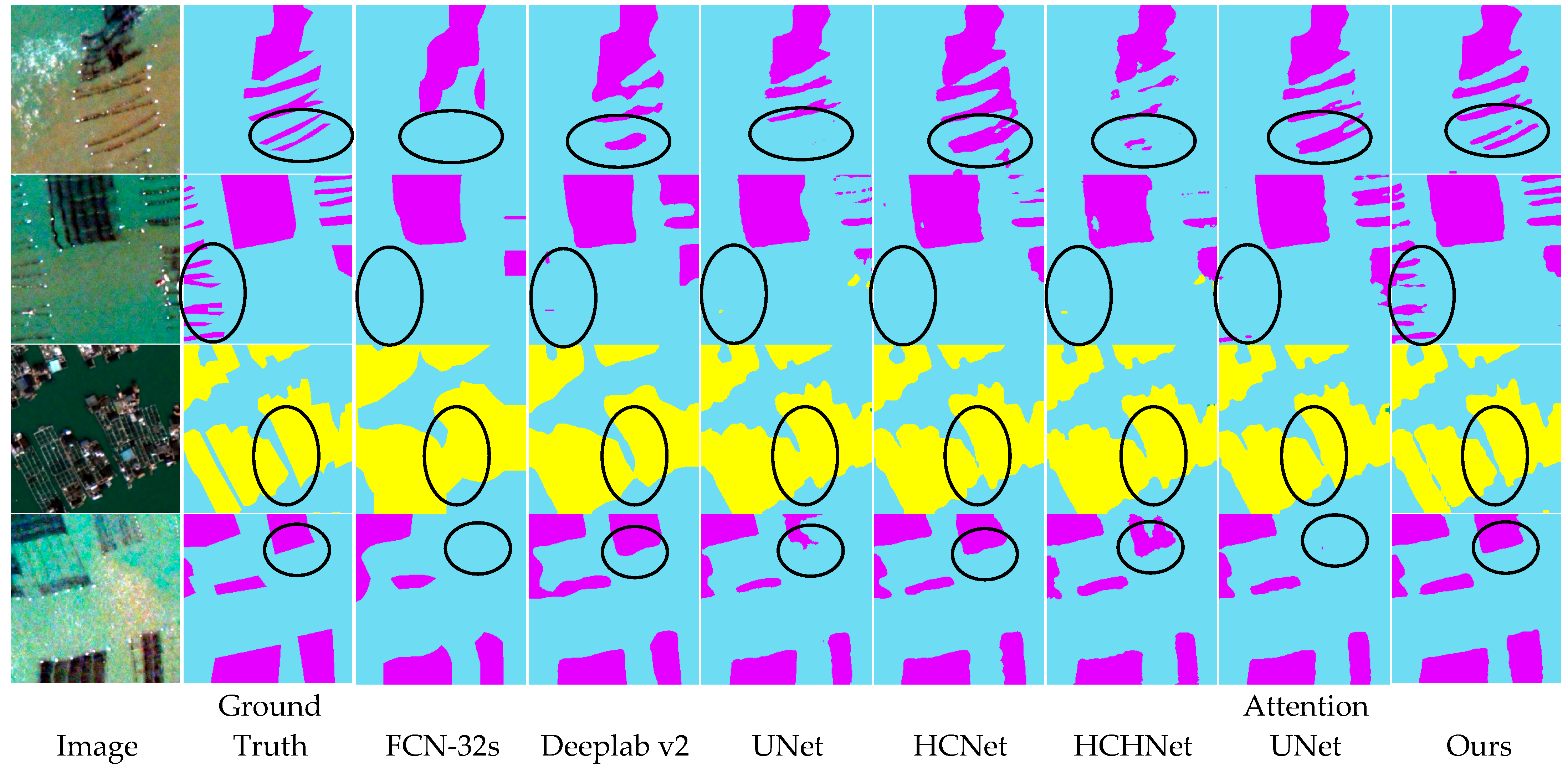
To further illustrate the differences of the evaluation metrics, we also visually compared the classification results from various methods. As shown in Figure 7, benefiting from the combination of local features and global semantic information, our proposed TCNet accurately delineated the boundary of RCA and CCA. In contrast, due to the lack of effective global information and refinement of detailed information, FCN-32s can only identify the main parts of large RCA or CCA, resulting in the lowest accuracy values. As the relatively weak in acquiring global information, UNet, Attention UNet, and HCHNet cannot accurately identify the RCA and CCA in complex marine environments. Meanwhile, without the benefits of any long span connection, Deeplab V2 can hardly delineate the details of RCA or CCA.

4.2. Transformer vs. Our Approach

Apart from the CNN-based methods, we also compared our proposed methods with the Transformer-based methods (Table 2). Compared with the pure Transformer-based models, such as SETR, Swin-UNet, and Segformer, our proposed TCNet can largely improve the accuracy values, with an improvement of 2.7–12.6% in terms of IoU. The Swin-UNet, Segformer, and TransUNet obtained similar accuracy values, with an IoU value of nearly 86.0%. The SETR achieved the lowest accuracy values, with an IoU value of lower than 80.0%.
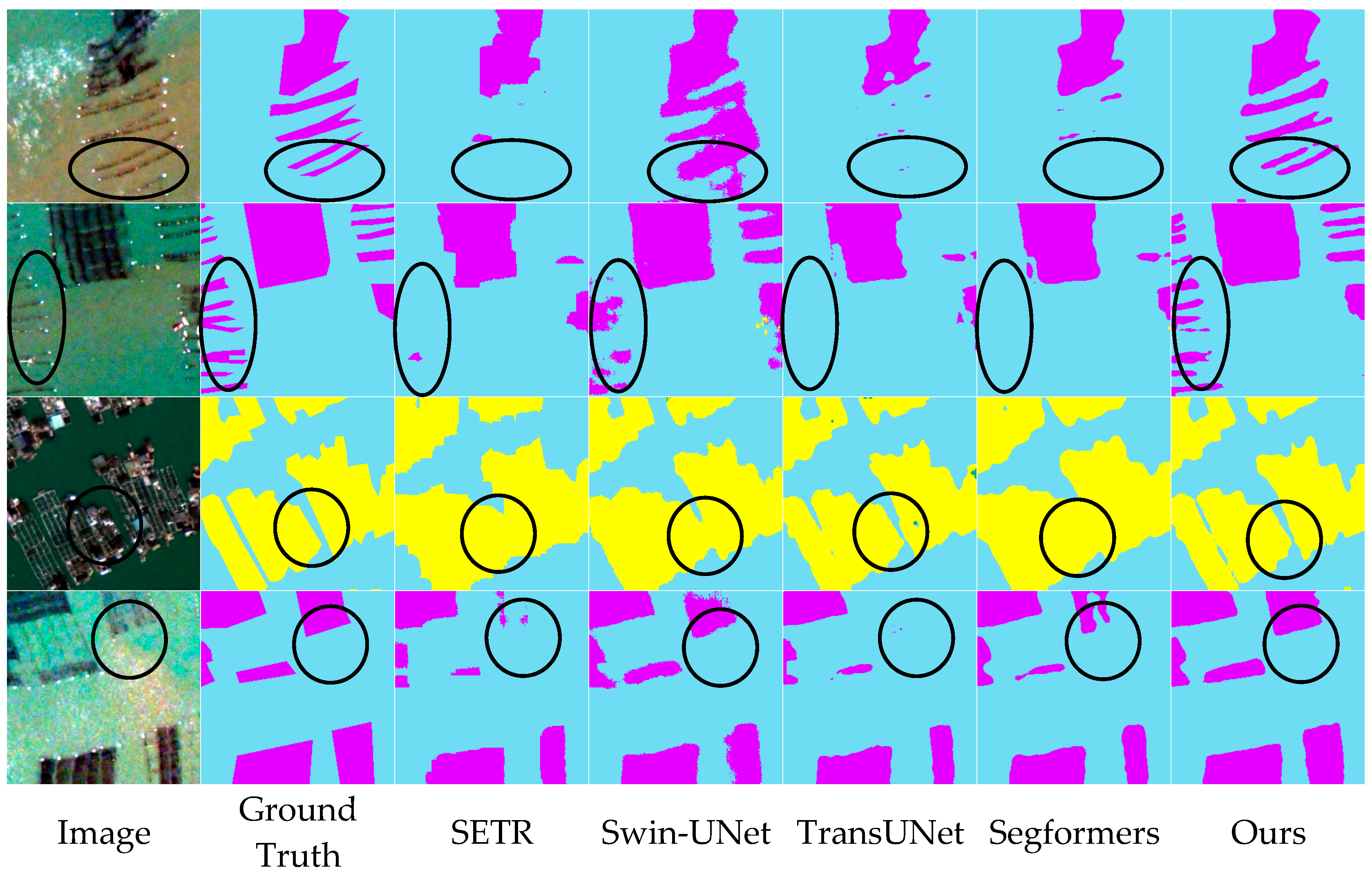
Meanwhile, as shown in Figure 8, we also compared the classification results from different Transformer-based models. Benefiting from the acquired effective global semantic information from Transformer layer, the SETR, Swin-UNet, Segformers, and TCNet can even effectively identify some of the submerged RCA. By combining the CNN-based structure in encoder, TransUNet and TCNet can extract more detailed boundaries of RCA and CCA. Compared with other models, TCNet can obtain the best performance in complex marine environments by combining local features from CNN and global semantic information from the proposed hierarchical lightweight Transformer module.

5. Discussion

5.1. Integrating Transformer and CNN for Semantic Segmentation

In recent years, there have been several attempts to utilize the Transformer architecture for global information extraction [33]. Due to its powerful sequence-to-sequence modeling capabilities, the Transformer has achieved state-of-the-art results on fundamental vision tasks [44,51,54]. However, when dealing with the confusing marine objects in complex marine environments, it is still a challenge to combine the advantages of Transformer for capturing global context and CNN for modeling local details in a complementary way. The first problem is that the computational complexity of Transformer-based encoders is much higher than that of CNN-based encoders due to their square-complexity self-attention mechanism [33]. This significantly limits their potential and feasibility for monitoring of marine aquaculture areas from VHSR images. The second problem is the semantic gap between local features from CNN and global scale features from Transformer. Direct concatenation of these features may cause misalignment of features from CNN and Transformer [55].
To solve these problems, our proposed TCNet mainly contributes in two aspects. First, different with the traditional state-of-the-art Transformer modules, such as ViT [44] SETR [51], and Swin Transformer [56], the lightweight Transformer module in our methods can largely reduce computational costs by using a progressive reduction process. As shown in Figure 9, SC-MSA reduce the spatial resolution of original “K” and “V” before the self-attention process, which largely reduce the computation costs compared with other traditional Transformer modules. Benefiting from such effective process, the module has more advantages, such as: Firstly, it can generate feature maps with different scales at different stages in our hierarchical structures, which can effectively capture the dependencies of marine aquaculture areas with its surrounding waters; secondly, it can be used to deal with high-resolution feature maps with limited computational costs, which is more suitable for the semantic segmentation of VHSR images. Additionally, we used a lightweight backbone, i.e., VGG-16, as its encoder and developed a hierarchical lightweight Transformer module in our study.
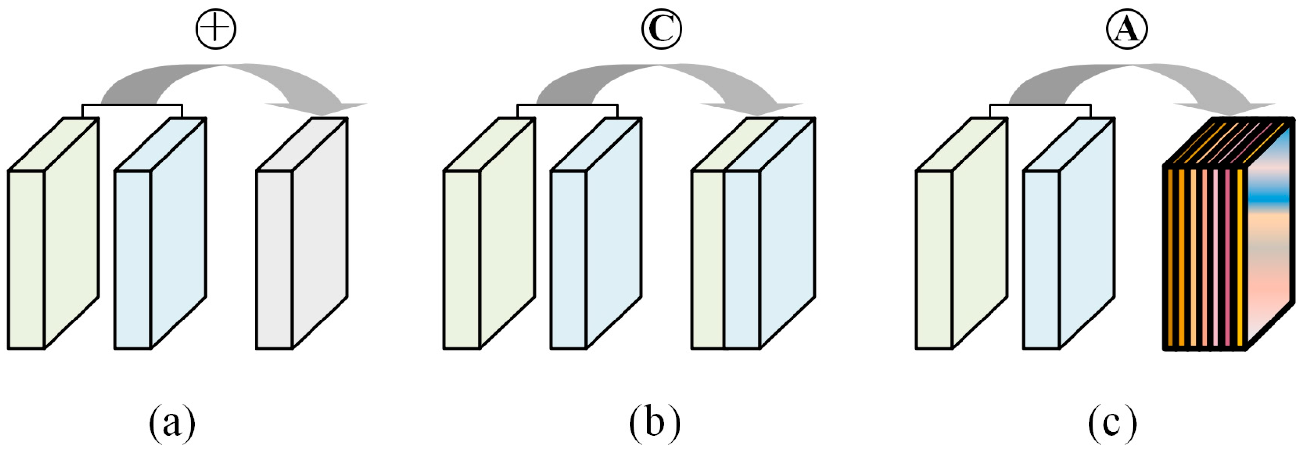
Furthermore, in contrast to the existing fusion of direct adding [55,57,58] or concatenation fashion [59], we proposed to use an attention-based module to aggregate the multi-scale features gradually (see Figure 10). The attention-based module, which can automatically assign importance score to each pixel of the features, allows the decoder to suppress noise in the encoder and focus on the most useful parts of the local features. In other words, such a structure was expected to suppress features of waves or turbid waters in the complex marine environment, and to focus on the details of marine aquaculture areas.

5.2. Additional Spectral Bands Analysis

Satellite imagery typically comprises multiple spectral bands. For example, VHSR satellites imagery (IKNOS, QuickBirds, GF-2, etc.) generally contains four multispectral bands (Blue, Green, Red, and Near-infrared). In contrast, WV2 imageries contain eight bands. All the additional bands are designed for the mapping of detailed coastal and vegetation types, such as mapping of plants stress, coastal water quality, bathymetry, etc. [60]. To investigate the capacity of the additional multispectral bands for the mapping of marine aquaculture areas, we tested the impact of additional band compositions on the performance of our TCNet on the testing dataset.
As shown in Table 3, the absence of additional bands caused a drop in distinguishing different types of the marine aquaculture areas (2.8%). Moreover, when the additional bands were removed, there was a 4.1% drop in the IoU value for CCA. One of the main reasons for this is that these additional bands, especially the band 6 and 8, showed larger differences between CCA and other land covers (see Figure 11). In contrast, the IoU value of RCA showed a slight drop (1.5%). This is because most of the additional bands (such as band 1, 6, and 8) showed a similar spectrum differentiation with the adjacent existing bands for the RCA and its surrounding sea water.
In general, full spectral bands are ideal configurations for the mapping of marine aquaculture areas. Meanwhile, with a slight drop in IoU values (2.8%), our proposed can also effectively capture the spatial information of mariculture areas from the four bands imagery at global scale, such as shape and texture, for the classification.

5.3. Ablation Analysis

To further evaluate the contributions of different structures in TCNet, we conducted the ablation experiments in this study (Table 4). In the experiments, we first constructed the baseline model by removing the hierarchical lightweight Transformer module and feature space refinement structures in TCNet. Then, we gradually added the hierarchical lightweight Transformer module and the feature space refinement structures for comparison.
As shown in Table 4, the classification accuracy value gradually improved by adding different structures. As a pure FCN-based model, which combines advantages of long-span connections in the decoder and atrous convolution in the encoder, the baseline model achieved a relatively high IoU value of 88.9%. Benefiting from the effective global information, the proposed hierarchical lightweight Transformer module can significantly improve the classification performance, with an improvement of nearly 1.5% in terms of IoU value. Meanwhile, the proposed FSR structure can also improve the classification values further.

5.4. Advantages and Limitations

In this study, our proposed TCNet mainly included three carefully designed structures: encoder based on CNN, hierarchical lightweight Transformer, and detailed structure refinement. The encoder was employed in our TCNet due to its fast convergence and reduced memory consumption. Benefiting from the hierarchical lightweight Transformer, TCNet was able to generate feature maps with different scales at different stages, which effectively captured the dependencies of marine aquaculture areas with its surrounding waters. Additionally, such a structure can effectively be used to deal with high-resolution features, which is more suitable for the extraction of marine targets from VHSR images. After that, by combining the detailed structure refinement structures, TCNet can effectively recover the local details of marine aquaculture areas while maintaining the global context. As a result, the proposed TCNet allowed the network to retain both fine spatial details and global representations to the maximum extent, resulting in an improved performance for the mapping of marine aquaculture areas.
Meanwhile, there were several limitations for our proposed TCNet. Firstly, due to the limitation of optical images, our methods can only decline the marine aquaculture that floats near the sea surface from VHSR images. Therefore, a future study that focuses on the extraction of bottom sowing culture of algae or scallop, which performs farming directly in the sea floor [61], is still needed. In addition, as such methods still rely on a large number of manually annotate samples, it is still valuable to explore some semi-supervised methods for the training process [62].

6. Conclusions

In this study, we proposed a Transformer–CNN hybrid Network for marine aquaculture mapping in complex marine environments from VHSR images. To deal with the associated complexities and challenges, our proposed TCNet focused on three important aspects: (1) a variant version of VGG-16 based encoder, which was designed to effectively extract high-dimensional and abstract features from input images; (2) the hierarchical lightweight Transformer module, which can be employed to extract the global semantic information from input features; (3) the detailed structure refinement structure, which can gradually recover the details of marine aquaculture areas by utilizing refined features from shallow layers.
The experimental results further validated the effectiveness and advantages of TCNet, with an IoU value of 90.9. Compared with other state-of-the-art FCN or Transformer-based methods, our methods can significantly improve the classification performance both visually and quantitatively.
Future studies may focus on testing our proposed methods on other types of land covers or computer vision tasks in complex environments, such as the classification or detection of roads, buildings, and trees in urban areas. Meanwhile, as such methods still rely on a large number of labels, it is also valuable to explore some semi-supervised methods for the training process. In addition, our methods can only decline the marine aquaculture that floats near the sea surface from VHSR images. Mapping methods of the mariculture that grows on the seafloor are still needed in the future.

Supplementary Materials

The following supporting information can be downloaded at: https://www.mdpi.com/article/10.3390/rs15184406/s1, Table S1: Confusion matrix for the testing dataset using our proposed TCNet; Figure S1: Loss and accuracy curves of TCNet for the traning process.

Author Contributions

Funding acquisition, Y.F., X.B. and P.W.; Investigation, F.G.; Methodology, Y.F.; Software, W.Z.; Visualization, X.B.; Writing—original draft, Y.F.; Writing—review and editing, P.W. All authors have read and agreed to the published version of the manuscript.

Funding

This research was funded by the National Natural Science Foundation of China, grant numbers 42101404 and 42107498; and the National Social Science Fund of China, grant number 20BTJ045.

Data Availability Statement

The labels used to train the model can be found on GitHub at the following link: https://github.com/yyong-fu/TCNet (accessed on 1 September 2023).

Acknowledgments

We would like to thank the support of Open Fund of State Laboratory of Agricultural Remote Sensing and Information Technology of Zhejiang Province.

Conflicts of Interest

The authors declare no conflict of interest.

References

  1. FAO. The State of World Fisheries and Aquaculture 2022: Towards Blue Transformation; FAO: Rome, Italy, 2022; pp. 3–4. [Google Scholar]
  2. Gentry, R.R.; Froehlich, H.E.; Grimm, D.; Kareiva, P.; Parke, M.; Rust, M.; Gaines, S.D.; Halpern, B.S. Mapping the global potential for marine aquaculture. Nat. Ecol. Evol. 2017, 1, 1317–1324. [Google Scholar] [CrossRef]
  3. Tovar, A.; Moreno, C.; Mánuel-Vez, M.P.; García-Vargas, M. Environmental impacts of intensive aquaculture in marine waters. Water Res. 2000, 34, 334–342. [Google Scholar] [CrossRef]
  4. Rubio-Portillo, E.; Villamor, A.; Fernandez-Gonzalez, V.; Antón, J.; Sanchez-Jerez, P. Exploring changes in bacterial communities to assess the influence of fish farming on marine sediments. Aquaculture 2019, 506, 459–464. [Google Scholar] [CrossRef]
  5. Rigos, G.; Katharios, P. Pathological obstacles of newly-introduced fish species in Mediterranean mariculture: A review. Rev. Fish Biol. Fish. 2010, 20, 47–70. [Google Scholar] [CrossRef]
  6. Lillesand, T.; Kiefer, R.W.; Chipman, J. Remote Sensing and Image Interpretation, 5th ed.; John Wiley & Sons: Hobokan, NJ, USA, 2004; pp. 42–44. [Google Scholar]
  7. Cheng, J.; Jia, N.; Chen, R.S.; Guo, X.A.; Ge, J.Z.; Zhou, F.C. High-Resolution Mapping of Seaweed Aquaculture along the Jiangsu Coast of China Using Google Earth Engine (2016–2022). Remote Sens. 2022, 14, 6202. [Google Scholar] [CrossRef]
  8. Geng, J.; Fan, J.; Wang, H. Weighted Fusion-Based Representation Classifiers for Marine Floating Raft Detection of SAR Images. IEEE Geosci. Remote Sens. 2017, 14, 444–448. [Google Scholar] [CrossRef]
  9. Zheng, Y.; Wu, J.; Wang, A.; Chen, J. Object-and pixel-based classifications of macroalgae farming area with high spatial resolution imagery. Geocarto Int. 2017, 33, 1048–1063. [Google Scholar] [CrossRef]
  10. Zheng, Y.H.; Duarte, C.M.; Chen, J.; Li, D.; Lou, Z.H.; Wu, J.P. Remote sensing mapping of macroalgal farms by modifying thresholds in the classification tree. Geocarto Int. 2019, 34, 1098–1108. [Google Scholar] [CrossRef]
  11. Wang, M.; Cui, Q.; Wang, J.; Ming, D.; Lv, G. Raft cultivation area extraction from high resolution remote sensing imagery by fusing multi-scale region-line primitive association features. Isprs J. Photogramm. 2017, 123, 104–113. [Google Scholar] [CrossRef]
  12. Fu, Y.; Deng, J.; Ye, Z.; Gan, M.; Wang, K.; Wu, J.; Yang, W.; Xiao, G. Coastal aquaculture mapping from very high spatial resolution imagery by combining object-based neighbor features. Sustainability 2019, 11, 637. [Google Scholar] [CrossRef]
  13. Fu, Y.; Ye, Z.; Deng, J.; Zheng, X.; Huang, Y.; Yang, W.; Wang, Y.; Wang, K. Finer Resolution Mapping of Marine Aquaculture Areas Using WorldView-2 Imagery and a Hierarchical Cascade Convolutional Neural Network. Remote Sens. 2019, 11, 1678. [Google Scholar] [CrossRef]
  14. Fu, Y.Y.; Deng, J.S.; Wang, H.Q.; Comber, A.; Yang, W.; Wu, W.Q.; You, S.X.; Lin, Y.; Wang, K. A new satellite-derived dataset for marine aquaculture areas in China’s coastal region. Earth Syst. Sci. Data 2021, 13, 1829–1842. [Google Scholar] [CrossRef]
  15. Shi, T.; Xu, Q.; Zou, Z.; Shi, Z. Automatic Raft Labeling for Remote Sensing Images via Dual-Scale Homogeneous Convolutional Neural Network. Remote Sens. 2018, 10, 1130. [Google Scholar] [CrossRef]
  16. Cui, B.E.; Fei, D.; Shao, G.H.; Lu, Y.; Chu, J.L. Extracting Raft Aquaculture Areas from Remote Sensing Images via an Improved U-Net with a PSE Structure. Remote Sens. 2019, 11, 2053. [Google Scholar] [CrossRef]
  17. Lu, Y.M.; Shao, W.; Sun, J. Extraction of Offshore Aquaculture Areas from Medium-Resolution Remote Sensing Images Based on Deep Learning. Remote Sens. 2021, 13, 3854. [Google Scholar] [CrossRef]
  18. Fu, Y.Y.; You, S.C.; Zhang, S.J.; Cao, K.; Zhang, J.H.; Wang, P.; Bi, X.; Gao, F.; Li, F.Z. Marine aquaculture mapping using GF-1 WFV satellite images and full resolution cascade convolutional neural network. Int. J. Digit Earth 2022, 15, 2048–2061. [Google Scholar] [CrossRef]
  19. Blaschke, T.; Hay, G.J.; Kelly, M.; Lang, S.; Hofmann, P.; Addink, E.; Feitosa, R.Q.; van der Meer, F.; van der Werff, H.; van Coillie, F.; et al. Geographic Object-Based Image Analysis—Towards a new paradigm. Isprs. J. Photogramm. 2014, 87, 180–191. [Google Scholar] [CrossRef]
  20. Shelhamer, E.; Long, J.; Darrell, T. Fully Convolutional Networks for Semantic Segmentation. IEEE Trans. Pattern Anal. Mach. Intell. 2017, 39, 640–651. [Google Scholar] [CrossRef]
  21. Yuan, Q.Q.; Shen, H.F.; Li, T.W.; Li, Z.W.; Li, S.W.; Jiang, Y.; Xu, H.Z.; Tan, W.W.; Yang, Q.Q.; Wang, J.W.; et al. Deep learning in environmental remote sensing: Achievements and challenges. Remote Sens. Env. 2020, 241, 111716. [Google Scholar] [CrossRef]
  22. Zhu, X.X.; Tuia, D.; Mou, L.; Xia, G.S.; Zhang, L.; Xu, F.; Fraundorfer, F. Deep Learning in Remote Sensing: A Comprehensive Review and List of Resources. IEEE Geosci. Remote Sens. Mag. 2017, 5, 8–36. [Google Scholar] [CrossRef]
  23. Lecun, Y.; Bengio, Y.; Hinton, G. Deep learning. Nature 2015, 521, 436–444. [Google Scholar] [CrossRef]
  24. Bengio, Y.; Courville, A.; Vincent, P. Representation Learning: A Review and New Perspectives. IEEE Trans. Pattern Anal. Mach. Intell. 2013, 35, 1798–1828. [Google Scholar] [CrossRef] [PubMed]
  25. Gao, Y.H.; Zhang, M.M.; Wang, J.J.; Li, W. Cross-Scale Mixing Attention for Multisource Remote Sensing Data Fusion and Classification. IEEE Trans. Geosci. Remote 2023, 61, 5507815. [Google Scholar] [CrossRef]
  26. Gao, Y.H.; Li, W.; Zhang, M.M.; Wang, J.B.; Sun, W.W.; Tao, R.; Du, Q. Hyperspectral and Multispectral Classification for Coastal Wetland Using Depthwise Feature Interaction Network. IEEE Trans. Geosci. Remote 2022, 60, 5512615. [Google Scholar] [CrossRef]
  27. Gao, Y.H.; Zhang, M.M.; Li, W.; Song, X.K.; Jiang, X.Y.; Ma, Y.Q. Adversarial Complementary Learning for Multisource Remote Sensing Classification. IEEE Trans. Geosci. Remote 2023, 61, 5505613. [Google Scholar] [CrossRef]
  28. Li, W.; Gao, Y.H.; Zhang, M.M.; Tao, R.; Du, Q. Asymmetric Feature Fusion Network for Hyperspectral and SAR Image Classification. IEEE Trans. Neur. Net. Lear. 2022, 1–14. [Google Scholar] [CrossRef]
  29. Peng, C.; Zhang, X.Y.; Yu, G.; Luo, G.M.; Sun, J. Large Kernel Matters—Improve Semantic Segmentation by Global Convolutional Network. In Proceedings of the 2017 IEEE Conference on Computer Vision and Pattern Recognition (CVPR), Honolulu, HI, USA, 21–26 July 2017; pp. 1743–1751. [Google Scholar]
  30. Chen, L.-C.; Papandreou, G.; Kokkinos, I.; Murphy, K.; Yuille, A.L. DeepLab: Semantic Image Segmentation with Deep Convolutional Nets, Atrous Convolution, and Fully Connected CRFs. IEEE Trans. Pattern Anal. Mach. Intell. 2018, 40, 834–848. [Google Scholar] [CrossRef]
  31. Zhao, H.; Shi, J.; Qi, X.; Wang, X.; Jia, J. Pyramid scene parsing network. In Proceedings of the 2017 IEEE Conference on Computer Vision and Pattern Recognition (CVPR), Honolulu, HI, USA, 21–26 July 2017; pp. 6230–6239. [Google Scholar]
  32. Wang, X.L.; Girshick, R.; Gupta, A.; He, K.M. Non-local Neural Networks. In Proceedings of the 2018 IEEE/CVF Conference on Computer Vision and Pattern Recognition, Salt Lake City, UT, USA, 18–23 June 2018; pp. 7794–7803. [Google Scholar]
  33. Vaswani, A.; Shazeer, N.; Parmar, N.; Uszkoreit, J.; Jones, L.; Gomez, A.N.; Kaiser, L.; Polosukhin, I. Attention Is All You Need. In Proceedings of the Adv Neur In, Long Beach, CA, USA, 4–9 December 2017; pp. 600–610. [Google Scholar]
  34. Ronneberger, O.; Fischer, P.; Brox, T. U-Net: Convolutional Networks for Biomedical Image Segmentation. In Proceedings of the Medical Image Computing and Computer-Assisted Intervention (MICCAI 2015), Munich, Germany, 5–9 October 2015; pp. 234–241. [Google Scholar]
  35. Hariharan, B.; Arbeláez, P.; Girshick, R.; Malik, J. Hypercolumns for object segmentation and fine-grained localization. In Proceedings of the 2015 IEEE Conference on Computer Vision and Pattern Recognition (CVPR), Boston, MA, USA, 7–12 June 2015; pp. 447–456. [Google Scholar]
  36. Pinheiro, P.O.; Lin, T.Y.; Collobert, R.; Dollár, P. Learning to refine object segments. In Proceedings of the European Conference on Computer Vision 2016, Amsterdam, The Netherlands, 8–16 October 2016; pp. 75–91. [Google Scholar]
  37. Noh, H.; Hong, S.; Han, B. Learning deconvolution network for semantic segmentation. In Proceedings of the 2015 IEEE International Conference on Computer Vision (ICCV), Santiago, Chile, 7–13 December 2015; pp. 1520–1528. [Google Scholar]
  38. Badrinarayanan, V.; Kendall, A.; Cipolla, R. SegNet: A Deep Convolutional Encoder-Decoder Architecture for Image Segmentation. IEEE Trans. Pattern Anal. Mach. Intell. 2017, 39, 2481–2495. [Google Scholar] [CrossRef]
  39. Updike, T.; Comp, C. Radiometric Use of WorldView-2 Imagery; DigitalGlobe: Westminster, CO, USA, 2010; pp. 1–17. [Google Scholar]
  40. Lin, C.; Wu, C.C.; Tsogt, K.; Ouyang, Y.C.; Chang, C.I. Effects of atmospheric correction and pansharpening on LULC classification accuracy using WorldView-2 imagery. Inf. Process. Agric. 2015, 2, 25–36. [Google Scholar] [CrossRef]
  41. Simonyan, K.; Zisserman, A. Very Deep Convolutional Networks for Large-Scale Image Recognition. arXiv 2015, arXiv:1409.1556. [Google Scholar] [CrossRef]
  42. Chen, J.; Lu, Y.; Yu, Q.; Luo, X.; Adeli, E.; Wang, Y.; Lu, L.; Yuille, A.L.; Zhou, Y. TransUNet: Transformers Make Strong Encoders for Medical Image Segmentation. arXiv 2021, arXiv:2102.04306. [Google Scholar] [CrossRef]
  43. Wang, W.H.; Xie, E.Z.; Li, X.; Fan, D.P.; Song, K.T.; Liang, D.; Lu, T.; Luo, P.; Shao, L. PVT v2: Improved baselines with Pyramid Vision Transformer. Comput. Vis. Media 2022, 8, 415–424. [Google Scholar] [CrossRef]
  44. Dosovitskiy, A.; Beyer, L.; Kolesnikov, A.; Weissenborn, D.; Zhai, X.; Unterthiner, T.; Dehghani, M.; Minderer, M.; Heigold, G.; Gelly, S.; et al. An Image is Worth 16x16 Words: Transformers for Image Recognition at Scale. arXiv 2020, arXiv:2010.11929. [Google Scholar] [CrossRef]
  45. Islam, M.A.; Jia, S.; Bruce, N.D.B. How Much Position Information Do Convolutional Neural Networks Encode? arXiv 2020, arXiv:2001.08248. [Google Scholar] [CrossRef]
  46. Chu, X.; Tian, Z.; Zhang, B.; Wang, X.; Shen, C. Conditional Positional Encodings for Vision Transformers. arXiv 2021, arXiv:2102.10882. [Google Scholar] [CrossRef]
  47. Hendrycks, D.; Gimpel, K. Gaussian Error Linear Units (GELUs). arXiv 2016, arXiv:1606.08415. [Google Scholar] [CrossRef]
  48. Zhang, Y.; Qiu, Z.; Yao, T.; Liu, D.; Mei, T. Fully Convolutional Adaptation Networks for Semantic Segmentation. In Proceedings of the 2018 IEEE/CVF Conference on Computer Vision and Pattern Recognition, Salt Lake City, UT, USA, 18–23 June 2018; pp. 3431–3440. [Google Scholar]
  49. Fu, J.; Liu, J.; Tian, H.J.; Li, Y.; Bao, Y.J.; Fang, Z.W.; Lu, H.Q. Dual Attention Network for Scene Segmentation. In Proceedings of the 2019 IEEE/CVF Conference on Computer Vision and Pattern Recognition (CVPR), Long Beach, CA, USA, 15–20 June 2019; pp. 3141–3149. [Google Scholar]
  50. Schlemper, J.; Oktay, O.; Schaap, M.; Heinrich, M.; Kainz, B.; Glocker, B.; Rueckert, D. Attention gated networks: Learning to leverage salient regions in medical images. Med. Image Anal. 2019, 53, 197–207. [Google Scholar] [CrossRef]
  51. Zheng, S.X.; Lu, J.C.; Zhao, H.S.; Zhu, X.T.; Luo, Z.K.; Wang, Y.B.; Fu, Y.W.; Feng, J.F.; Xiang, T.; Torr, P.H.S.; et al. Rethinking Semantic Segmentation from a Sequence-to-Sequence Perspective with Transformers. In Proceedings of the 2021 IEEE/CVF Conference on Computer Vision and Pattern Recognition (CVPR), Nashville, TN, USA, 20–25 June 2021; pp. 6877–6886. [Google Scholar]
  52. Cao, H.; Wang, Y.; Chen, J.; Jiang, D.; Zhang, X.; Tian, Q.; Wang, M. Swin-Unet: Unet-Like Pure Transformer for Medical Image Segmentation. In Proceedings of the ECCV 2022, Tel Aviv, Israel, 23–27 October 2022; pp. 205–218. [Google Scholar]
  53. Xie, E.Z.; Wang, W.H.; Yu, Z.D.; Anandkumar, A.; Alvarez, J.M.; Luo, P. SegFormer: Simple and Efficient Design for Semantic Segmentation with Transformers. arXiv 2021, arXiv:2105.15203. [Google Scholar] [CrossRef]
  54. Zhu, X.; Su, W.; Lu, L.; Li, B.; Wang, X.; Dai, J. Deformable DETR: Deformable Transformers for End-to-End Object Detection. arXiv 2021, arXiv:2010.04159. [Google Scholar] [CrossRef]
  55. Peng, Z.; Huang, W.; Gu, S.; Xie, L.; Wang, Y.; Jiao, J.; Ye, Q. Conformer: Local Features Coupling Global Representations for Visual Recognition. arXiv 2021, arXiv:2105.03889. [Google Scholar] [CrossRef]
  56. Liu, Z.; Lin, Y.T.; Cao, Y.; Hu, H.; Wei, Y.X.; Zhang, Z.; Lin, S.; Guo, B.N. Swin Transformer: Hierarchical Vision Transformer using Shifted Windows. In Proceedings of the 2021 IEEE/CVF International Conference on Computer Vision (ICCV), Montreal, QC, Canada, 10–17 October 2021; pp. 9992–10002. [Google Scholar]
  57. Carion, N.; Massa, F.; Synnaeve, G.; Usunier, N.; Kirillov, A.; Zagoruyko, S. End-to-End Object Detection with Transformers. arXiv 2020, arXiv:2005.12872. [Google Scholar] [CrossRef]
  58. Jamali, A.; Roy, S.K.; Ghamisi, P. WetMapFormer: A unified deep CNN and vision transformer for complex wetland mapping. Int. J. Appl. Earth Obs. 2023, 120, 103333. [Google Scholar] [CrossRef]
  59. Yuan, F.N.; Zhang, Z.X.; Fang, Z.J. An effective CNN and Transformer complementary network for medical image segmentation. Pattern Recogn. 2023, 136, 109228. [Google Scholar] [CrossRef]
  60. Marchisio, G.; Pacifici, F.; Padwick, C. On the Relative Predictive Value of the New Spectral Bands in the Worldview-2 Sensor. In Proceedings of the 2010 IEEE International Geoscience and Remote Sensing Symposium, Honolulu, HI, USA, 25–30 July 2010; pp. 2723–2726. [Google Scholar]
  61. Maeda-Martinez, A.N.; Ormart, P.; Mendez, L.; Acosta, B.; Sicard, M.T. Scallop growout using a new bottom-culture system. Aquaculture 2000, 189, 73–84. [Google Scholar] [CrossRef]
  62. Yang, X.L.; Song, Z.X.; King, I.; Xu, Z.L. A Survey on Deep Semi-Supervised Learning. IEEE Trans. Knowl. Data En. 2023, 35, 8934–8954. [Google Scholar] [CrossRef]
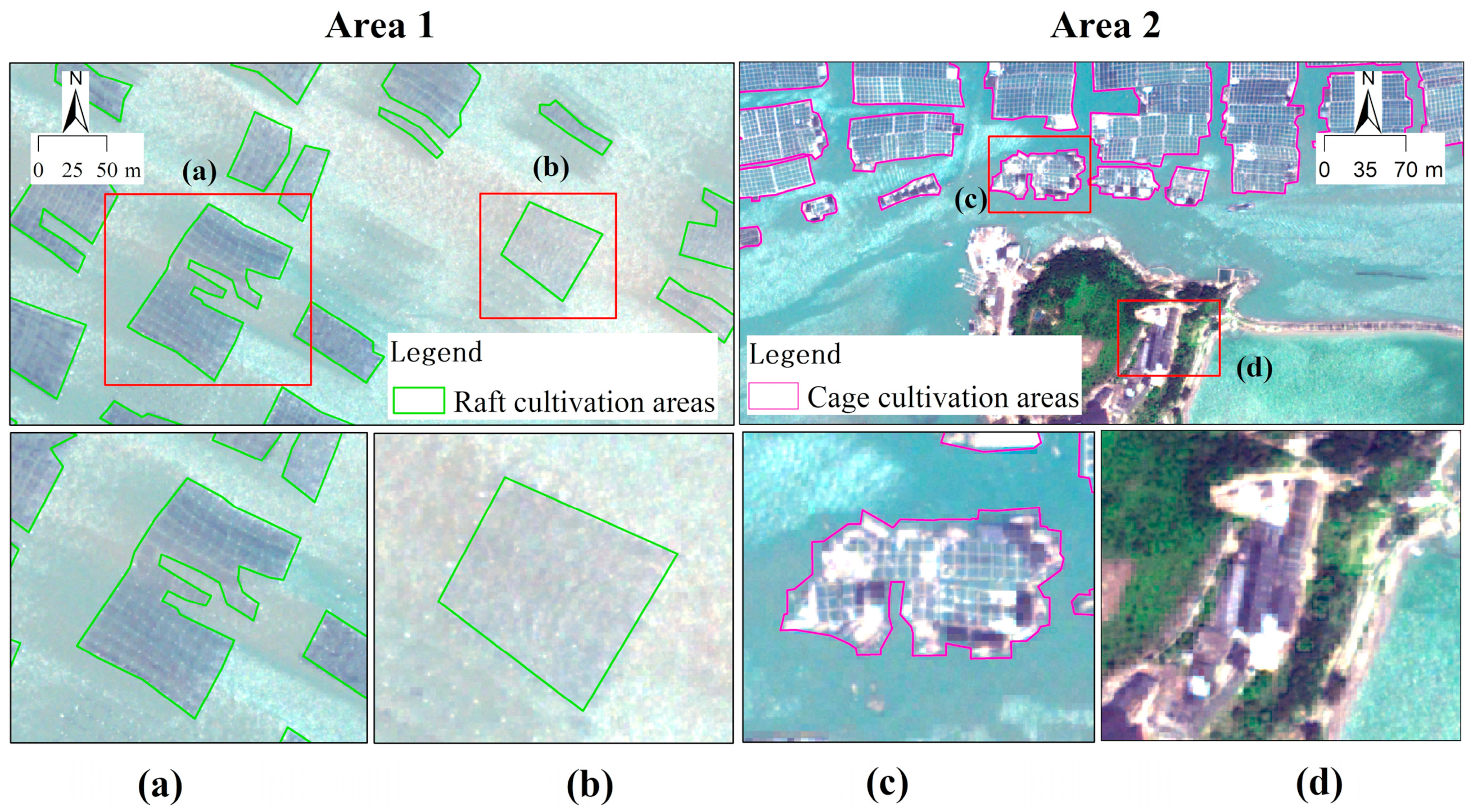
Figure 1. Marine aquaculture areas extraction with inter-class similarity and intra-class variance. (a,b) are of the same class but presented in totally different shapes, sizes, and colors. (b) shows similar texture and color with the surrounding waves. Pixels in the cage cultivation areas of (c) are of the same class but presented in totally different color. Part of the (c,d) are of different classes but share similar structural patterns.
Remotesensing 15 04406 g001
Figure 2. Location and imagery used in our study. Typical images of the raft cultivation area (RCA, (a,b)) and cage cultivation area (CCA, (c,d)) are shown in the right part.
Remotesensing 15 04406 g002
Figure 3. Flowchart of our study. B, G, R, Nir1, CB, Y, RE, and Nir2 represents the band of blue, green, red, NIR1, coastal blue, yellow, and NIR2 of the WorldView-2 imagery, respectively.
Remotesensing 15 04406 g003
Figure 4. The overall framework of our proposed Transformer–CNN hybrid Network (TCNet). The color of red, yellow, green, and blue represents RCA, CCA, land, and sea areas, respectively.
Remotesensing 15 04406 g004
Figure 5. Structure of the Transformer layer in our study. ‘SC-MSA’ represents the spatial condensed Multi-Head Attention. ‘DC-FFN’ represents the depth-wise convolution feed-forward network. ‘FC’ represents a fully connected layer.
Remotesensing 15 04406 g005
Figure 6. The process of traditional patch embedding (a) and the overlapping patch embedding (b) in our study.
Remotesensing 15 04406 g006
Figure 7. Segmentation results of different FCN-based models in complex marine environments. The color of red, yellow, green, and blue represents RCA, CCA, land, and sea areas, respectively. The black circles indicate that the our proposed TCNet obtains better performance.
Remotesensing 15 04406 g007
Figure 8. Segmentation results of different Transformer-based models in complex marine environments. The color of red, yellow, green, and blue represents RCA, CCA, land, and sea areas, respectively.
Remotesensing 15 04406 g008
Figure 9. Comparison of the traditional MSA and SC-MSA in our study. ‘MSA’ represents the spatial condensed Multi-Head Attention. ‘SC-MSA’ represents the spatial condensed Multi-Head Attention.
Remotesensing 15 04406 g009
Figure 10. Comparison of different fusion style. (a) and ‘⊕’ represent the addition fusion strategy. (b) and ‘©’ represent the concatenation fusion strategy. (c) and ‘ ’ represent our proposed attention fusion strategy.
Remotesensing 15 04406 g010
Figure 11. Digital number values of different land covers in this study. Band numbers correspond to multi-spectrum bands of WorldView-2 imagery.
Remotesensing 15 04406 g011
Table 1. Quantitative comparison of different FCN-based models on the testing dataset. The best accuracy values are in bold. And the second best are underlined.
MethodsRCACCAMean
F1-ScoreIoUF1-ScoreIoUF1-ScoreIoU
FCN-32s0.890.800.900.830.900.81
Deeplab v20.930.860.940.890.930.88
UNet0.920.860.950.910.940.89
HCNet0.930.870.950.910.940.89
HCHNet0.910.840.930.860.920.85
Attention UNet0.930.870.960.920.950.90
Ours-TCNet0.930.880.970.940.950.91
Table 2. Quantitative comparison of different Transformer-based models on the testing dataset.
MethodsRCACCAMean
F1-ScoreIoUF1-ScoreIoUF1-ScoreIoU
SETR0.890.810.860.760.880.78
Swin-UNet0.910.830.940.880.920.86
TransUNet0.920.850.960.920.940.88
Segformers0.920.850.930.880.930.87
Ours-TCNet0.930.880.970.940.950.91
Table 3. Performance of the TCNet trained on training dataset without (TCNet-4)/with (TCNet-8) additional band composition.
MethodsRCACCAMean
F1-Score
(%)
IoU
(%)
F1-Score
(%)
IoU
(%)
F1-Score
(%)
IoU
(%)
TCNet-492.686.394.789.993.788.1
TCNet-893.587.896.994.095.290.9
Table 4. Ablation experiment of our proposed TCNet. ‘+HLT’ represents aggregating the proposed hierarchical lightweight Transformer module. ‘+HLT + FSR’ represents aggregating the hierarchical lightweight Transformer module and the feature space refinement structure.
MethodsRCACCAMean
F1-Score
(%)
IoU
(%)
F1-Score
(%)
IoU
(%)
F1-Score
(%)
IoU
(%)
Baseline92.986.895.391.094.188.9
+HLT93.487.796.493.195.090.4
+HLT + FSR93.587.896.994.095.290.9
Disclaimer/Publisher’s Note: The statements, opinions and data contained in all publications are solely those of the individual author(s) and contributor(s) and not of MDPI and/or the editor(s). MDPI and/or the editor(s) disclaim responsibility for any injury to people or property resulting from any ideas, methods, instructions or products referred to in the content.