Understanding Road Traffic Evolution in an Urbanizing Context through Statistical and Geospatial Analysis

Abstract

Urbanization, an accelerated process, is inherently coupled with complex issues, including the evolution of road traffic systems. This diversity in urbanization and transport infrastructure largely hinges on economic status and geographic positioning across cities. Leveraging the capabilities of remote sensing and Geographic Information Systems (GIS) in processing geospatial big data, this paper evaluates the urbanization level (UL) and road traffic level (RTL) in 212 prefecture-level cities using statistical and geospatial grid data. We aim to dissect the impact of UL on RTL, thus highlighting the specific challenges and opportunities across regions and pinpointing optimal urban development models. Our findings demonstrate (1) rapid development in UL across all cities, juxtaposed with a surge and then stagnation in RTL; (2) a positive correlation between UL and RTL that grows over time but weakens in later stages; (3) differentiated development models in different city tiers and regions; and (4) region-specific development models and optimization policies aimed at enhancing the symbiosis of urbanization and road traffic. This study underscores the pivotal role of the integration of statistical and geospatial data in understanding the dynamic intersection of urbanization and road traffic systems.

1. Introduction

Urbanization’s evolution leads to significant shifts in tangible aspects such as urban spatial structures, including land elements, infrastructure, transportation networks, and statistical indicators that reflect economic and social progress [1]. In the modern industrialization context, urbanization has exhibited various patterns over a development process that follows an “S” curve divided into three stages: primary, intermediate, and advanced, and each urbanization stage mirrors distinct social scenarios [2]. In some countries, national resources are concentrated in a few rapidly developing cities with strategic locations; these cities drive the movement of elements like population, land, and capital. As a result, cities progress through various urbanization stages, leading to significant regional differences. Urbanization reflects other different social characteristics, including urban sprawl [3], economic growth, technological advancements, and infrastructure improvements in transportation, tourism, health, and education [4].

As statistical data, spatiotemporal big data, and remote sensing technology advance, more comprehensive methods are emerging to measure urbanization. Current evaluations of urbanization are mainly conducted across dimensions like population structure, economic structure, and land use, primarily using panel data, while some scholars employ night light data or other geospatial sources [5]. Moreover, improving remote sensing accuracy and machine learning has enabled higher spatiotemporal resolution in land use classification data. The Annual China Land Cover Dataset (CLCD) includes China’s annual land cover information from 1985 to 2021, greatly aiding land urbanization measurements [6]. WorldPop data have made it easier to determine urban populations in non-administrative units and conduct urbanization studies on a spatial scale [7,8].

The United Nations Statistical Commission’s endorsement of the Degree of Urbanization for delimiting urban and rural areas allows for the measurement of global urbanization on a 1 km grid scale [9]. Many urbanization-related studies based on spatiotemporal big data have emerged, such as in situ urbanization in inland non-metropolitan rural settlements [10]. The intertwined relationships between urbanization and environmental factors like energy consumption, energy efficiency, carbon emissions, sustainable land use, and ecosystem services have been explored to illuminate a greener, more sustainable urbanization pathway [11,12,13,14,15].

Additionally, the spillover of public infrastructure has also led to a series of effects that promote the urbanization process [16,17], and they are interrelated and synergistically affect sustainable development [18,19]. Improving infrastructure is an essential part of realizing urbanization, social equity, and eco-friendly cities [20,21], as well as promoting regional development, the circulation of elements, and convenience for residents [22,23]. In addition, various studies have found a bidirectional relationship between investment in infrastructure and the economic development of a region [23].

Transport infrastructure has been observed to exhibit a significant positive correlation with urbanization. It is closely associated with non-agricultural economic development, the agglomeration of people, and an increase in built-up areas, which is one of the most critical infrastructures, accounting for considerable investment [24]. With the improvements in urbanization, the mobility and agglomeration of elements and products continue to increase. The transportation infrastructure as a circulation carrier directly affects the regular operation of the entire urban social system and the realization of urban functions [25], as well as connecting elements, increasing the efficiency of urban operations and promoting a series of urban activities [26]. Mohmand et al. [27] confirmed the short-term causal relationship between Pakistan’s economic growth, transportation infrastructure, fuel consumption, and transportation carbon emissions. From the perspective of the local area, surrounding areas, and the entire country, transportation infrastructure construction effectively promotes the economic development of the local and surrounding areas [28]. From the two dimensions of country and region, using panel data to analyze the impact of transportation construction on agriculture, industry, and service industries, Cantos et al. [28] proved that road transportation construction significantly increases GDP growth in various sectors. Some studies elaborate from a more microscopic perspective, highlighting that transportation infrastructure can reduce transportation costs and shorten labor travel time and communication costs between different regions, thereby increasing labor productivity [29]. Many scholars mentioned that transportation helps promote economic growth, or economic growth promotes transportation from the national, interstate, and interprovincial dimensions [28].

With the progression of urbanization, the infrastructure and road traffic systems within cities are undergoing significant transformations. Few studies have revealed the changes and spatial heterogeneity of road traffic during urbanization at the national scale, in different city types, and with time series dimensions. Therefore, this paper further studies the relationship between road traffic and urbanization in the urban size to reveal the impact of urbanization on road traffic levels in different cities (development levels, regional differences) and summarize their characteristics and change patterns.

China, with a vast territory, has undergone tremendous development and changes in the past few decades, and the transport infrastructure is a crucial factor that causes many economic and social differences [30]. Cities in different regions are at various stages of urbanization. In addition, cities also represent different transportation positions, such as transportation hubs, coastal cities, capitals, and economic centers. The impact of urbanization on road traffic construction varies over time and region. This paper takes the urbanization and road traffic infrastructure of 212 prefecture-level cities in China as the research object, evaluates the level of urbanization and road traffic through the combination of statistical data and spatiotemporal geographic data, and explores their change patterns and interaction mechanisms through GIS platforms and econometric statistical models, which aims at (1) exhibiting the spatiotemporal dynamics of urbanization and road traffic of 212 cities; (2) exploring the temporal and spatial heterogeneity in the impact of urbanization on road traffic; (3) helping decision-makers locate the spatiotemporal development patterns of road traffic infrastructure during urbanization; and (4) promoting positive interaction between road transport and urbanization to provide planners with an empirical base on regional collaborative development.

2. Materials and Methods

2.1. Research Framework

As the process of urbanization is staged, in different stages, the road transport infrastructure’ response to urbanization differs. A particular city corresponds to its location (a certain period of urbanization). Therefore, this research mainly focuses on diverse city road transport infrastructure in different urbanization processes (different geographical conditions and positioning). As the direct carrier of vehicles, road transport infrastructure is the most basic means for cities to connect production factors and passenger and freight transportation. Consequently, empirical research on the relationship between transport infrastructure and urbanization under a spatiotemporal sequence has theoretical and practical significance.

To reflect the interrelation between China’s road transport infrastructure and urbanization, the research framework in this article is studied from a temporal scale and a spatial scale. The temporal scale is yearly from 2009 to 2020. On the spatial scale, according to “The 13th Five-Year Plan for the Development of Modern Comprehensive Transportation System”, “The Central Committee of the Communist Party of China and the State Council issued opinions on establishing a more effective new mechanism for coordinated regional development”, and “Chinese Geographical Division”, the sample cities are divided into five categories: Central Traffic Hub, Municipality, Northeast Capital City, Northwestern Inland city, Pearl River Delta, and Yangtze River Delta. Moreover, the city-level judgment comes from the “new first-tier city summit”, which evaluates 337 Chinese cities from five perspectives: the concentration of commercial resources, the urban hub, the activity of urban residents, the diversity of lifestyles, and the future plasticity of cities. The algorithm framework is as follows: the weights of the primary index are scored by the expert committee of the New First-Tier Cities Institute, while the data below the secondary index are analyzed by principal component analysis [31]. Based on the availability and completeness of the data, a total of 212 cities were selected for research, including 17 first-tier cities, 28 second-tier cities, 53 third-tier cities, 63 fourth-tier cities, and 51 fifth-tier 51 cities; the main cities of each tier are presented in

Table 1. Main cities of each tier.

City Tier	City Name
First-tier	Beijing, Shanghai, Guangzhou, Shenzhen, Chengdu, Chongqing, Wuhan, Xi’an, Tianjin, Nanjing, etc.
Second-tier	Wuxi, Foshan, Hefei, Dalian, Fuzhou, Xiamen, Harbin, Jinan, Wenzhou, etc.
Third-tier	Shantou, Huzhou, Yancheng, Baoding, Zhenjiang, Luoyang, Taizhou, Urumqi, etc.
Fourth-tier	Shaoguan, Changde, Lu’an, Shanwei, Xining, Maoming, Zhumadian, Xingtai, Nanchong, etc.
Fifth-tier	Guang’an, Tianshui, Yan’an, Baicheng, Ya’an, Hanzhong, Panzhihua, Ankang, Liaoyuan, etc.

. Judging from the distribution of city levels (Figure 1), most first-tier cities are in the east, or some inland capital cities, while the cities of the latter few tiers are primarily in the central and western regions.

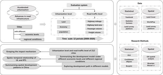
This paper determines the urbanization level (UL) by built-up land, economy, and population. The road traffic level (RTL) is determined by highway mileage, land area, passenger volume, and freight volume. Our study is focused on the impact mechanisms of urbanization on road transport infrastructure in different cities and periods as the three main parts of the study. In detail, the framework of the study (Figure 2) is (1) establishing the evaluation systems of urbanization and road traffic; (2) calculating the level of urbanization and level of road transport infrastructure of China’s 212 cities to understand their temporal and spatial distribution characteristics; (3) locating the development model of road infrastructure under different levels of urbanization; this paper distinguishes and analyzes the relationship between urbanization and transportation under different regional characteristics and economic levels; (4) summarizing the different development models in China and finding the optimal city examples under each model.

2.2. Data

This study is primarily based on statistical data and spatial data. Statistical data are mainly collected from various statistical yearbooks. The raster data in this study include land cover data and spatial population data. The data details are shown in

Table 2. Indicators for assessing the farmland fragmentation.

Type	Indicators	Format	Source
Statistical	GDP	Text	2010–2021 China Statistical Yearbook, China City Statistical Yearbook
	Production value of secondary and tertiary industries	Text	2010–2021 China Statistical Yearbook, China City Statistical Yearbook
	Permanent population, permanent urban population	Text	2010–2021 China Statistical Yearbook, China City Statistical Yearbook
	Highway mileage, highway passenger and freight volume	Text	2010–2021 China Statistical Yearbook, China City Statistical Yearbook
	Highway land area	Text	Land survey results sharing application service platform (China)
	Population	Text	Statistics bureaus of prefectural-level cities
Spatial	Land cover dataset (Annual China Land Cover Dataset, CLCD)	Raster	https://doi.org/10.5281/zenodo.5816591 (accessed on 1 July 2023)
	WorldPop Global Project Population Data	Raster	http://www.worldpop.org.uk (accessed on 1 July 2023)
	Relief Degree of Land Surface	Raster	https://doi.org/10.3974/geodb.2018.03.16.V1 (accessed on 1 July 2023)

. The WorldPop population Distribution Map is a continuous annual dataset with a spatial resolution of 100 m published by the WorldPop project. It is mainly based on administrative unit-based census data and multi-source data such as land cover, night lighting, topography, and distance to roads and rivers from 2000 to 2020, spatialized with the help of a random forest machine learning algorithm [8]. In this paper, Worldpop data for each year at the scale of the study area are obtained from the Google Earth Engine platform. The CLCD is a continuous annual dataset with a spatial resolution of 30 m, which is generated based on all available Landsat SR data on Google Earth Engine, with an average accuracy of 79.30%.

In this study, to make data of different dimensions comparable, the data are standardized by dividing by the maximum value of all time periods. The standardized values should be between 0 and 1. Additionally, raster data are extracted to administrative unit scale using the zonal statistics tool of ArcGIS. When the image element sizes or alignments of the region boundaries and the value raster are different, the image elements between the region boundaries and the value raster will not be able to overlay each other perfectly. The tool will internally adjust the raster to achieve a perfect pixel overlay. This triggers an internal resampling before the region operation is performed.

2.3. Urbanization Level Evaluation System

Urbanization is a complex system transformation process [32], and scholars of various disciplines have offered explanations from their professional perspectives. Demography emphasizes the migration and concentration of the rural population to cities, increasing the proportion of the urban population. Economics emphasizes the process of transition and transformation from the rural economy to the urban economy. Geography emphasizes cities’ continuous concentration of people and industries, transforming the regional landscape from rural to urban. A single discipline cannot define urbanization. Therefore, this article establishes an evaluation system of UL from the three aspects of economic urbanization rate (EU), population urbanization rate (PU), and land urbanization rate (LU).

2.3.1. Economic Urbanization Rate

The development of non-agricultural industries is one of the essential characteristics of economic urbanization. The urbanization process benefits from industrial development, and the deepening of the urbanization process is attributed to the rise and prosperity of the tertiary industry. The secondary and tertiary sectors show the degree of development of urban non-agricultural industries from different aspects, so the added value of secondary and tertiary sectors as a percentage of GDP can reasonably and accurately represent the proper level of economic urbanization. In summary, the economic urbanization rate formula is as follows:

$$\mathrm{E}\mathrm{U}=\frac{\mathrm{S}\mathrm{T}\mathrm{P}}{\mathrm{G}\mathrm{D}\mathrm{P}}\times 100\%$$

(1)

where the EU represents the economic urbanization rate, STP represents the second and third output value, and GDP represents the gross domestic product.

2.3.2. Population Urbanization Rate

The proportion of the urban population in the total population can evaluate the UL of the population. The permanent population refers to the number of people who have resided in the prefecture level city for more than half a year at the end of that year. This article uses the permanent population instead of the urban population. The population urbanization rate formula is as follows:

$$\mathrm{P}\mathrm{U}=\frac{\mathrm{P}\mathrm{U}\mathrm{P}}{\mathrm{U}\mathrm{P}\mathrm{R}}\times 100\%$$

(2)

where $\mathrm{P}\mathrm{U}$ represents the population urbanization rate, PUP represents the permanent urban population, and PR represents the total permanent population.

2.3.3. Land Urbanization Rate

The urban functional area usually refers to the area covered by urban work, housing, entertainment, and medical functions, with the built-up area as the core and one working day as the cycle. It also includes that the built-up land area has close social and economic ties and a trend of integration in the city’s outer regions [33]. Therefore, the built-up land area can be the most suitable basic unit for judging land urbanization. More prominent is the concept of land use, which directly reflects the change of land from agriculture to non-agriculture, which also includes the urbanization of areas such as the “village in the city” process. Its scale and changes represent urban land’s absolute level and progress, so this indicator is most suitable for evaluating the land urbanization rate. This article extracts the built-up land area from the CLCD dataset. In summary, the calculation formula for the land urbanization rate is as follows:

$$\mathrm{L}\mathrm{U}=\frac{\mathrm{U}\mathrm{C}\mathrm{L}}{\mathrm{U}\mathrm{A}}\times 100\%$$

(3)

where $\mathrm{L}\mathrm{U}$ is the land urbanization rate, UCL is the urban built-up land area, and UA is the urban area (administrative area).

2.3.4. UL Index Weight Calculation

This study ultimately chose the equal weight method to calculate the weights of UL and RTL, compared with the principal component analysis method and the entropy weight method. The principal component analysis method starts with downscaling and simplifying the data by transforming the original multiple indicators with correlation into a few representative composite indicators [34]. The entropy weighting method determines the weights by the numerical characteristics of the data. For a certain indicator, the entropy value can be used to determine the degree of dispersion of the indicator. The smaller the information entropy value, the greater the degree of dispersion of the indicator, and the greater the impact of the indicator on comprehensive evaluation [35]. In this paper, we consider that each indicator of UL and RTL contributes equally to the calculations. To mitigate the impact of subjective weight assignments and to uniformly represent urbanization attributes across economy, population, and land sectors, a holistic urbanization score is computed by allocating equal weights to each dimension. The calculation formula for the urbanization level is as follows:

$$\mathrm{U}\mathrm{L}=\frac{1}{3}\times (\mathrm{E}\mathrm{U}+\mathrm{P}\mathrm{U}+\mathrm{L}\mathrm{U})$$

(4)

2.4. RTL Evaluation System

2.4.1. Selection of Road Traffic Construction Indicators

Highways in China are multi-lane roads designed for high-speed automobile travel in separate directions and lanes, with all the access controlled. The design speed is 80 to 120 km per hour. Highways usually run through the entire administrative boundary and are connected to surrounding cities, reflecting the level of regional road construction and the degree of connection with surrounding cities.

Mileage is the most fundamental indicator for judging the development of transportation construction, and it can directly reflect the level of transportation construction. The continuous increase in highway mileage reflects road transportation construction’s constant development and improvement. In this study, highway mileage is considered, and the area of highway land should be listed as one of the research indicators, which will reflect the development of road transportation more objectively. Passenger and freight volumes reflect the transportation capacity of a mode of transportation and are the primary means of economic and social circulation of human and material resources. Although road passenger traffic has experienced a downward trend in recent years, it still accounted for 79% of the total passenger traffic in 2017. Although the proportion of road freight in the total freight volume has not significantly changed, its freight volume has remained at about 76% of the total freight volume. Therefore, this paper has established an indicator system to evaluate the RTL, as shown in

Table 3. Indicator system of RTL.

System	Index	Definition	Unit
Road traffic level	Highway density (HD)	Mileage opened to traffic per unit land area	km/km2
	Percentage of road land (PRL)	The proportion of highway land to a total area	%
	Passenger volume per area (PVPA)	Highway passenger traffic per unit area of land	Ten thousand people/km2
	Freight volume per area (FVPA)	Road freight volume per unit area of land	10,000 tons/km2

.

2.4.2. RTL Index Weight Calculation

For the same considerations as in determining UL weights, to equally reflect the characteristics of road traffic in terms of HD, PRL, PVPA, and FVPA, the RTL is calculated by summing equal weights. The calculation formula for the urbanization level is as follows:

$$\mathrm{R}\mathrm{T}\mathrm{L}=0.25\times (\mathrm{H}\mathrm{D}+\mathrm{P}\mathrm{R}\mathrm{L}+\mathrm{P}\mathrm{V}\mathrm{P}\mathrm{A}+\mathrm{F}\mathrm{V}\mathrm{P}\mathrm{A})$$

(5)

2.5. Analysis Methods for the Impact of Urbanization on RTL

This paper uses the ordinary least squares method (OLS) to explore the relationship between UL and RTL. In addition, considering the impact of GDP and terrain factors on road traffic construction, GDP per capita and Relief Degree of Land Surface (RDLS) are the control variables. This paper explores the impact of UL, PU, EU, and LU on RTL over eight years.

We employed a method that replaces the core independent variable with WorldPop data to assess the robustness of our regression model’s outcomes. We extracted the average population of all pixels in each city to characterize the level of urbanization. We employed the same OLS model to explore its impact on RTL.

In addition, this paper applies the bivariate Moran’s I to reflect the relationship between UL and RTL from the perspective of the spatial agglomeration effect. Moran’s index is a spatial measurement model that considers spatial agglomeration characteristics and helps measure the spatial correlation between urbanization and traffic levels. Moran’s I > 0 represents a positive correlation between the variables; Moran’s I < 0 represents a negative correlation, and Moran’s I = 0 means that the significance test is not passed and the variables are distributed randomly.

3. Results

3.1. Evaluation Result Analysis of Urbanization and Road Traffic

The upper limit, lower limit, median, and upper and lower quartiles of the evaluation results for each year are displayed in Figure 3. The values outside the boundary are outliers, mainly cities with high scores. Looking into the boxes, the RTL in these 12 years is approximately clustered around 0.15, distributed from 0 to 0.4, and continues to grow from 2009 to 2020. The UL is approximately clustered around 0.5, distributed from 0.1 to 0.8, and continues to grow from 2009 to 2020. From the appearance of the outliers, the most frequent outlier in UL is Shenzhen, while outliers in the transportation level include Shenzhen, Shanghai, Dongguan, Guangzhou, Wuxi, and Changzhou in the first five years. As the frontier of reform and opening up, Shenzhen has long realized comprehensive industrialization and urbanization. The entire population of Shenzhen was urbanized. Therefore, Shenzhen’s road infrastructure and urbanization levels are ahead of China’s. Based on the high outlier scores of certain cities, these cities are primarily located along the coasts of the Pearl and Yangtze Rivers.

From 2009 to 2020 (Figure 4), the UL of cities over the years showed a situation of first-tier> second-tier> third-tier> fourth-tier> fifth-tier. Among them, the UL of third-, fourth-, and fifth-tier cities are far lower than those of first-tier and second-tier cities. The trends in the UL of various tiers are showing continued growth. Gaps between each tier of cities remain constant over time. As for RTL, the first-tier cities are much higher than others, while the third- and fourth-tier cities score relatively close. From the perspective of changes, from 2009 to 2020, the RTL in most tiers of cities showed an increasing trend, while it decreased in the last 2 years. Among them, the first-tier and second-tier cities grew the most, while the others presented moderate growth. Overall, the RTLs of all cities show rapid growth from 2009 to 2012, slowing down from 2012 to 2019, with a decline in the last year.

From the perspective of spatial distribution (Figure 5), the UL and RTL of each city present a decreasing trend from southeast to inland. The southeast coast shows a concentrated distribution of high values of UL and RTL, while several scattered inland provincial capitals have higher UL and RTL. First-tier and second-tier cities generally have a relatively high level of urbanization, while a few cities in the southwest and northwest have high UL, but RTL significantly lags.

3.2. The Impact Mechanisms of Urbanization on RTL

3.2.1. The Impact of UL on RTL

The results of the OLS model (

Table 4. Regression results of the impact of UL on RTL.

Variables	Year
	2009	2010	2011	2012	2013	2014	2015	2016	2017	2018	2019	2020
UL	0.4264 ***	0.4616 ***	0.5031 ***	0.5770 ***	0.6275 ***	0.6540 ***	0.6449 ***	0.5984 ***	0.5665 ***	0.6279 ***	0.5894 ***	0.5460 ***
	(0.0666)	(0.0643)	(0.0661)	(0.0650)	(0.0599)	(0.0625)	(0.0678)	(0.0681)	(0.0593)	(0.0586)	(0.0567)	(0.0651)
GDP per capita	−2.06 × 10−7	−3.11 × 10−7	−2.98 × 10−7	−4.53 × 10−7 *	−6.07 × 10−7 ***	−6.63 × 10−7 ***	−4.84 × 10−7 *	−2.54 × 10−7 *	1.01 × 10−8 ***	−2.70 × 10−7 *	−2.22 × 10−7	−2.48 × 10−7 *
	(3.73 × 10−7)	(3.13 × 10−7)	(2.73 × 10−7)	(2.20 × 10−7)	(1.69 × 10−7)	(1.79 × 10−7)	(1.92 × 10−7)	(1.89 × 10−7)	(1.55 × 10−9)	(1.13 × 10−7)	(1.17 × 10−7)	(1.18 × 10−7)
RDLS	−0.0355 ***	−0.0366 ***	−0.0368 ***	−0.0383 ***	−0.0359 ***	−0.0339 ***	−0.0329 ***	−0.0344 ***	−0.0339 ***	−0.0364 ***	−0.0325 ***	−0.0336 ***
	(0.0045)	(0.0049)	(0.0049)	(0.0051)	(0.0050)	(0.0049)	(0.0050)	(0.0053)	(0.0057)	(0.0056)	(0.0056)	(0.0057)
Constant	0.0364	−0.0442	−0.0615 *	−0.0856 **	−0.1058 ***	−0.1187 ***	−0.1242 ***	−0.1094 ***	−0.1075 ***	−0.1167 ***	−0.0974 ***	−0.0767 *
	(0.0265)	(0.0268)	(0.0286)	(0.0296)	(0.0291)	(0.0305)	(0.0331)	(0.0334)	(0.0334)	(0.0313)	(0.0312)	(0.0354)

*** p < 0.001, ** p < 0.01, * p < 0.05.

) indicate that UL has a significant positive impact on RTL. This positive effect gradually increased from 2009 to 2015 and weakened from 2016 to 2017 and from 2019 to 2020. RDLS significantly negatively impacts RTL; regions with high RDLS have lower RTL values. The impact of GDP per capita on RTL was significant from 2012 to 2018 but not significant at other times. In general, cities with a higher UL will have a higher RTL, and the promoting effect of UL on RTL increases in the early stage. With the further advancement of urbanization in the later stage, this promoting effect is weakening. Meanwhile, areas with a flat terrain are more conducive to improving RTL.

3.2.2. The Impact Mechanism of Different City Tiers

The distribution of the scatter plots and 95% confidence ellipses for each tier of cities (Figure 6) further reflects the different impact mechanisms of each city tier. It is observed that the characteristic points of each city are distributed near the diagonal line, showing that the two levels have a significant correlation. Tier-one cities have a high UL, but the RTL ranges from low to high, and the slope of the scatter is decreasing. Second-tier cities have changed dramatically in 12 years, almost catching up with first-tier cities in 2020. Third-, fourth-, and fifth-tier cities are generally in the lower left corner of the coordinate system. From 2009 to 2020, the scattered points of second- to fifth-tier cities kept moving slowly towards the upper right corner, which means there is still a big gap with first-tier cities. Generally, the gap between other tiers and tier-one cities is decreasing, and the positive relationship between UL and RTL is gradually increasing, but it decreases in 2020.

3.2.3. The Impact of Different Urbanization on RTL

The results of the OLS model (

Table 5. Regression results of the impact of PU on RTL.

Variables	Year
	2009	2010	2011	2012	2013	2014	2015	2016	2017	2018	2019	2020
PU	0.0510	0.0859	0.1063 *	0.1311 *	0.1923 **	0.2223 **	0.2406 **	0.2021 *	0.2823 ***	0.2771 ***	0.2367 ***	0.1658 **
	(0.0478)	(0.0473)	(0.0519)	(0.0581)	(0.0669)	(0.0707)	(0.0756)	(0.0793)	(0.0554)	(0.0697)	(0.0608)	(0.0595)
GDP per capita	1.19 × 10−7 *	8.19 × 10−7	7.02 × 10−7	6.01 × 10−7	2.63 × 10−7	1.04 × 10−7	1.75 × 10−7	4.03 × 10−7	5.91 × 10−9 ***	6.39 × 10−8	1.70 × 10−7	2.99 × 10−7
	(4.81 × 10−7)	(4.19 × 10−7)	(3.92 × 10−7)	(4.23 × 10−7)	(4.04 × 10−7)	(3.83 × 10−7)	(3.93 × 10−7)	(3.86 × 10−7)	(1.27 × 10−9)	(2.02 × 10−7)	(1.79 × 10−7)	(1.84 × 10−7)
RDLS	−0.0449 ***	−0.0477 ***	−0.0493 ***	−0.0532 ***	−0.0536 ***	−0.0538 ***	−0.0517 ***	−0.0517 ***	−0.0546 ***	−0.0565 ***	−0.0522 ***	−0.0531 ***
	(0.0052)	(0.0055)	(0.0057)	(0.0060)	(0.0059)	(0.0059)	(0.0061)	(0.0063)	(0.0006)	(0.0063)	(0.0059)	(0.0058)
Constant	0.1134 ***	0.1115 ***	0.1067 ***	0.1045 ***	0.0866 ***	0.0769 **	0.0615 *	0.0712 *	0.0515	0.0524	0.0676 *	0.0954 **
	(0.0168)	(0.0176)	(0.0195)	(0.0215)	(0.0244)	(0.0265)	(0.0287)	(0.0304)	(0.0315)	(0.0324)	(0.0309)	(0.0313)

*** p < 0.001, ** p < 0.01, * p < 0.05.

) demonstrate the impact of PU on RTL in eight years. From 2009 to 2012, the effects of PU on RTL were either not significant or weakly significant. From 2013 to 2020, PU significantly and positively promoted RTL. This facilitation has increased in previous years, being most significant in 2017 and decreasing from 2018 to 2020. RDLS also has a significant negative impact on RTL. The effect of GDP per capita on RTL is not substantial.

The results of the OLS model (

Table 6. Regression results of the impact of the EU on RTL.

Variables	Year
	2009	2010	2011	2012	2013	2014	2015	2016	2017	2018	2019	2020
EU	0.1179	0.1655 *	0.2337 **	0.2717 *	0.3009 **	0.3373 **	0.3511 **	0.3313 *	0.6102 ***	0.5132 ***	0.4993 ***	0.4721 ***
	(0.0811)	(0.0831)	(0.0895)	(0.1077)	(0.1088)	(0.1187)	(0.1220)	(0.1162)	(0.0922)	(0.0983)	(0.0863)	(0.0805)
GDP per capita	1.10 ×10−6 *	8.32 × 10−7	6.58 × 10−7	5.85 × 10−7	4.85 × 10−7	3.84 × 10−7	4.85 × 10−7	5.96 × 10−7	9.88 × 10−9 ***	2.31 × 10−7	2.07 × 10−7	1.40 × 10−7
	(5.46 × 10−7)	(4.74 × 10−7)	(4.37 × 10−7)	(4.84 × 10−7)	(4.35 × 10−7)	(4.18 × 10−7)	(4.23 × 10−7)	(3.84 × 10−7)	(1.75 × 10−9)	(2.05 × 10−7)	(1.96 × 10−7)	(1.96 × 10−7)
RDLS	−0.0454 ***	−0.0483 ***	−0.0501 ***	−0.0537 ***	−0.0540 ***	−0.0536 ***	−0.0518 ***	−0.0510 ***	−0.0552 ***	−0.0556 ***	−0.0512 ***	−0.0502 ***
	(0.0053)	(0.0056)	(0.0058)	(0.0060)	(0.0061)	(0.0059)	(0.0059)	(0.0060)	(0.0058)	(0.0060)	(0.0056)	(0.0056)
Constant	0.0381	0.0089	−0.0425	−0.0659	−0.0857	−0.1150	−0.1335	−0.1206	−0.3328 ***	−0.2598 ***	−0.2431 ***	−0.2118 ***
	(0.0576)	(0.0602)	(0.0652)	(0.0777)	(0.0797)	(0.0889)	(0.0906)	(0.0867)	(0.0812)	(0.0802)	(0.0707)	(0.0657)

*** p < 0.001, ** p < 0.01, * p < 0.05.

) demonstrate the impact of the EU on RTL from 2009 to 2020. In 2009, the relationship between the EU and RTL was insignificant; from 2010 to 2015, there was a significant positive effect, and the effect continually increased. In the later period, 2017–2020, the positive promotion of RTL by PU weakened, but there was still a significant positive effect. This indicates that transitioning the economy from agriculture to non-agricultural sectors can enhance RTL. Likewise, regions with flatter terrain are better suited for promoting RTL. While GDP per capita positively impacted RTL in 2009 and 2017, its influence was negligible in other years.

The results of the OLS model (

Table 7. Regression results of the impact of LU on RTL.

Variables	Year
	2009	2010	2011	2012	2013	2014	2015	2016	2017	2018	2019	2020
LU	0.3830 ***	0.3878 ***	0.3774 ***	0.4035 ***	0.3986 ***	0.3872 ***	0.3682 ***	0.3523 ***	0.3976 ***	0.3621 ***	0.3472 ***	0.3303 ***
	(0.0302)	(0.0318)	(0.0332)	(0.0346)	(0.0330)	(0.0317)	(0.0347)	(0.0336)	(0.0338)	(0.0278)	(0.0255)	(0.0335)
GDP per capita	3.69 × 10−7	3.11 × 10−7	3.59 × 10−7	3.13 × 10−7	2.30 × 10−7	2.04 × 10−7	3.21 × 10−7	3.86 × 10−7 *	1.13 × 10−8 ***	3.02 × 10−7 **	2.43 × 10−7 *	2.75 × 10−7 **
	(2.09 × 10−7)	(1.89 × 10−7)	(1.84 × 10−7)	(1.86 × 10−7)	(1.67 × 10−7)	(1.63 × 10−7)	(1.80 × 10−7)	(1.75 × 10−7)	(2.12 × 10−9)	(1.03 × 10−7)	(1.06 × 10−7)	(1.05 × 10−7)
RDLS	−0.0185 ***	−0.0197 ***	−0.0207 ***	−0.0212 ***	−0.0209 ***	−0.0211 ***	−0.0205 ***	−0.0213 ***	−0.0219 ***	−0.0229 ***	−0.0201 ***	−0.0197 ***
	(0.0031)	(0.0034)	(0.0037)	(0.0038)	(0.0038)	(0.0038)	(0.0040)	(0.0042)	(0.0043)	(0.0041)	(0.0042)	(0.0046)
Constant	0.0967 ***	0.1029 ***	0.1053 ***	0.1089 ***	0.1136 ***	0.1158 ***	0.1119 ***	0.1131 ***	0.1302 ***	0.1165 ***	0.1251 ***	0.1223 ***
	(0.0066)	(0.0075)	(0.0085)	(0.0091)	(0.0094)	(0.0094)	(0.0106)	(0.0105)	(0.0075)	(0.0103)	(0.0118)	(0.0121)

*** p < 0.001, ** p < 0.01, * p < 0.05.

) demonstrate the impact of LU on RTL from 2009 to 2020. LU has consistently had a significant positive effect on RTL over the 12 years. Distinct from other types of urbanization, LU initially had the most substantial impact in 2009 to 2012, and it continued to weaken after that. This suggests that in the early stages of urbanization, land transfer and spatial expansion of built-up land have a better effect on raising RTL. In the later stages of urbanization, this effect diminishes.

3.3. Robust Test of the Impact of Urbanization on RTL

To ensure the robustness of the research results, this article adopts the method of replacing core independent variables using the same model for robustness testing. The results in

Table 8. Regression results of the robust test.

Variables	Year
	2009	2010	2011	2012	2013	2014	2015	2016	2017	2018	2019	2020
WorldPop	0.0104 ***	0.0107 ***	0.0108 ***	0.0112 ***	0.0110 ***	0.0110 ***	0.0108 ***	0.0102 ***	0.0109 ***	0.0096 ***	0.0089 ***	0.0085 ***
	(0.0012)	(0.0013)	(0.0013)	(0.0014)	(0.0014)	(0.0015)	(0.0014)	(0.0014)	(0.0014)	(0.0015)	(0.0014)	(0.0008)
GDP per capita	5.09 × 10−7 *	4.22 × 10−7 *	4.19 × 10−7 *	3.87 × 10−7	3.05 × 10−7	2.30 × 10−7	3.00 × 10−7	3.43 × 10−7 *	3.94 × 10−9 *	2.55 × 10−7 *	1.89 × 10−7	2.20 × 10−7 **
	(2.33 × 10−7)	(2.10 × 10−7)	(1.97 × 10−7)	(2.04 × 10−7)	(1.81 × 10−7)	(1.65 × 10−7)	(1.70 × 10−7)	(1.66 × 10−7)	(1.63 × 10−9)	(1.07 × 10−7)	(1.09 × 10−7)	(1.13 × 10−7)
RDLS	−0.0294 ***	−0.0313 ***	−0.0322 ***	−0.0351 ***	−0.0360 ***	−0.0361 ***	−0.0350 ***	−0.0361 ***	−0.0402 ***	−0.0413 ***	−0.0392 ***	−0.0382 ***
	(0.0034)	(0.0036)	(0.0037)	(0.0039)	(0.0040)	(0.0041)	(0.0040)	(0.0043)	(0.0045)	(0.0047)	(0.0045)	(0.0041)
Constant	0.1087 ***	0.1160 ***	0.1191 ***	0.1265 ***	0.1337 ***	0.1373 ***	0.1343 ***	0.1378 ***	0.1609 ***	0.1505 ***	0.1616 ***	0.1580 ***
	(0.0070)	(0.0075)	(0.0081)	(0.0092)	(0.0094)	(0.0095)	(0.0096)	(0.0099)	(0.0079)	(0.0110)	(0.0115)	(0.0108)

*** p < 0.001, ** p < 0.01, * p < 0.05.

demonstrate that urbanization, as characterized by WorldPop data, has a significant positive effect on RTL. This positive effect is weakening in later stages of urbanization, similar to the impact of LU. This indicates that transitioning the economy from agriculture to non-agricultural sectors can enhance RTL. Likewise, regions with flatter terrain are better suited for promoting RTL. While GDP per capita has a mildly significant contribution to RTL most of the time.

3.4. Spatial Relationship between Urbanization and Transportation

The spatial distribution of both levels shows a precise alignment, characterized by a stepped gradient transitioning from the southeast to the northwest. Additionally, as depicted in Figure 7, geographical distribution and spatial spillover disparities are evident across China. Primarily, eastern coastal cities exhibit high UL values, while concurrently boasting high RTL values, including major cities like Beijing, Tianjin, and cities in the Pearl and Yangtze River Deltas. The figure further demonstrates the completeness of road transportation infrastructure in key inland hubs like Xi’an, Chengdu, and Zhengzhou. While various regions boast cities with developed transportation, cities with high UL predominantly reside along the eastern coast. Analysis of the results indicates that urban transport infrastructure significantly affects spillover effects: cities with developed road traffic typically have a higher UL value, influencing nearby cities. For instance, cities in Shanghai, Shandong, and Jiangsu with high traffic volumes can affect neighboring cities in Anhui and Henan provinces.

As the Bivariate Local Moran’s I visualized in Figure 7, where H-H represents high UL and high RTL aggregation, L-L represents low UL and low RTL aggregation, and H-L represents high UL and low RTL aggregation, L-H represents low UL and high RTL aggregation. It is evident that H-H areas are mainly concentrated in coastal areas such as the Yangtze River Delta, the Pearl River Delta, and Shandong Province. Moreover, there are L-L accumulations and H-L accumulations in inland areas, including the southwest, northwest, and northeast. This indicates that the RTL and UL in these areas are poor, and the H-L aggregation shows that these areas with developed urbanization have backward road transportation infrastructure.

3.5. Matching the Relationship of UL and RTL in Different Types of Cities

This study examines the urban context of China, considering the varied regional conditions, development stages, and other influencing factors across its cities. This analysis enables us to correlate levels of road traffic with urbanization stages across different cities. From individual city perspectives, we identified several cities that serve as regional exemplars and proposed various development models that are evident across China, as illustrated in Figure 8. Cities in the Pearl River Delta, including Guangzhou, Shenzhen, and Dongguan, exhibit the highest levels of urbanization and RTL. As a primary economic hub, Shanghai also ranks high on both metrics. Compared to other inland cities, provincial capital cities often act as transportation hubs and possess a higher RTL. For instance, Zhengzhou is the predominant transportation hub in the Central Plains of China. Cities in the Yangtze River Delta, being coastal and proximal to economic hubs, consistently rank at an elevated level. Despite being an inland municipality directly overseen by the Central Government, Chongqing lags in development compared to other municipalities. Northwestern Inland and Northeastern Capital cities’ high UL stems primarily from a dense urban population and expansive built-up areas. However, they face suboptimal traffic conditions and possess modest economic output.

In the eastern cities, the transportation infrastructure appears well developed. These cities should use their entire infrastructure to have a good spillover effect and drive regionally coordinated development. As a link between regions, central cities should play a good role in their value as a transportation hub, fully connect with big cities, and drive their development. For areas with backward transportation infrastructure, unquestioningly increasing investment in transportation facilities may not promote the process of urbanization, which needs to adapt to the development stage of the region. This paper believes that the progress of the two levels needs the stimulus of economic development and the promotion of multiple factors, and the two are complementary to each other.

4. Discussion

4.1. Main Achievements and Innovations

Remote sensing and geospatial data can effectively supplement statistical data and provide higher spatiotemporal resolution assessments of visualized surface processes such as urbanization. In this study, we assessed the evolutionary patterns of UL and RTL from a long time series as well as the changes in the mechanism of UL’s impact on RTL. This paper concludes that the effect of different types of urbanization on RTL varies across different time periods. After grasping the impact mechanisms at the national level, we generalized the development patterns of the typical districts from a regional perspective and captured the specific characteristics of the interactions between UL and RTL in the different sub-districts. Critically, this study bridges the gap in exploring the spatial and temporal heterogeneity of urbanization and road traffic at the prefecture-level city scale in China from a long time series.

4.2. Implications for Policy-Making

Urbanization has a significant positive effect on RTL, and this effect is realized as an increase and then a decrease, indicating that the promotion of RTL is weakening in the later stages of urbanization and that there is a slight saturation effect of road infrastructure development. The rise of RTL by PU and EU gradually increased on the time scale, while a slight weakening appeared later. Whereas the promotion of RTL by LU has been significant, this promotion has weakened over time. This suggests that the contribution of built-up land expansion to RTL has been waning. Decision-makers need to be aware of the diminishing role of the promotion of RTL by UL to rationalize the provision and layout of road transport facilities. In addition, advances in other transportation facilities, such as China’s railroads and airlines, have resulted in a declining share of road transportation at later stages of urbanization.

The factors that determine the UL and RTL of a city mainly include economic location and geographic location. This paper summarizes explicitly the development models of cities under different location conditions to seize their advantages and limitations and aims to provide suggestions for the development prospects of other cities (Figure 9). The development of urban agglomerations and road traffic are mutually reinforcing, and China’s current pattern of urbanization is inextricably linked to the vertical axis of Beijing– Pearl River Delta and Beijing–Yangtze River Delta–Pearl River Delta, the horizontal axis of Chengdu–Wuhan–Yangtze River Delta, which supports the main skeleton of the country’s comprehensive transportation network as well as metropolitan area construction. Based on the vision of China’s road network construction and the findings of this study, we propose the following policy recommendations.

First of all, cities such as China’s east coast H-H belt with vital openness and superior location conditions already have complete transportation infrastructure and a high level of urbanization. Since transportation is connected between cities, its spatial spillover benefits enable such cities to form developed urban agglomerations, such as Yangtze River Delta Urban Agglomerations and Pearl River Delta Urban Agglomeration. Such cities have entered the stage of tapping the potential of stock, where RTL has a tendency to stagnate or decline in later years. Policy-makers should pay attention to the intensive use of land, and tap into road traffic’s role in driving urbanization. At the same time, it will promote the integrated development of urban agglomerations based on complete road traffic.

Secondly, inland transportation hub cities like Zhengzhou, Xi’an, Changsha, and Chengdu also have relatively high UL and RTL. Such cities still have much room for development. They should promote the urbanization process with transportation infrastructure and act as regional hubs. The above two types of cities already have complete infrastructure. The priority job is internal optimization to achieve coordinated development of road transportation and urbanization, driving the growth of neighboring L-H cities, and promoting sustainable development in Central China.

Due to the disadvantages of geographical location and natural factors, the development of the Northwest H-L and L-L Zones and the Southwest L-L Zone is restricted. The construction of road traffic in these areas has enormous potential, and planners should reasonably deploy the construction of road networks to promote connectivity between lagging cities and other cities and drive regional development in the northwest and northeast regions. They should consider their resource utilization efficiency and take sustainable development instead of unquestioningly expanding and inefficient resource utilization. Finally, cities in northeast China that have historically developed industries, as the economic center of gravity shifts to the south, lose economic vitality. However, their geographic location is ideal and has sufficient land resources. Therefore, Northeast China should develop road traffic and drive regional economic growth.

4.3. Limitations and Uncertainties

Due to the availability of city-dimensional statistical data, it is impossible to obtain complete data on the permanent population of all prefecture-level cities; therefore, we selected relevant data for 212 cities. In future research, the data of all prefecture-level cities should be collected and studied more comprehensively and replaced by other types of data. The three indicators of economic, population, and land urbanization were considered. However, the connotation of the indicators was not explored deeply enough, resulting in the indicator system being too simple. Due to the limited ability to obtain national-scale, long-time series data, LU only considers the proportion of built-up land and fails to measure it at a finer scale, which may have limitations. The road traffic index does not consider factors such as road surface and road conditions inside the city. In the follow-up research, we can dig deeper into the connotations of urbanization and refine road traffic indicators to make the indicator selection more scientific and reasonable.

5. Conclusions

This paper establishes evaluation indicator systems for the level of urbanization from three aspects: land, economy, and population, and the level of RTL from four elements: highway mileage, highway land area, passenger volume, and freight volume. This paper grasps the spatiotemporal evolution of UL and RTL in 212 prefecture-level cities from 2009 to 2020 and the impact of different types of urbanization on RTL across different periods. The regression results were tested using WorldPop data. Different development patterns based on city tiers and regional disparities are clarified. The results demonstrate that (1) the UL of all cities is rapidly developing, while the RTL has significant growth in the early stage and stagnation in the later stage; the gap among different city tiers is significant. (2) UL has a significant positive promotional effect on RTL, and this effect increases over time and appears to weaken in the later stages. The promoting effect of PU and EU on RTL is first increasing and then decreasing, while LU continues to decrease. (3) Cities in different city tiers and regions have their unique development models; specifically, first-tier cities and the coastal cities have very high UL, and RTL is showing a saturation as well as a downward trend. Inland underdeveloped cities have a significant growth rate, and the increase in UL can continue to promote the increase in RTL. (4) The development models and optimization policies for various regions have been proposed to achieve a better interaction between urbanization and road traffic.

References

1. Seto, K.C.; Fragkias, M.; Güneralp, B.; Reilly, M.K. A meta-analysis of global urban land expansion. PLoS ONE 2011, 6, e23777. [Google Scholar] [CrossRef]
2. Northam, R.M. Urban Geography; John Wiley and Sons: Hoboken, NJ, USA, 1979. [Google Scholar]
3. Davis, J.C.; Henderson, J.V. Evidence on the political economy of the urbanization process. J. Urban Econ. 2003, 53, 98–125. [Google Scholar] [CrossRef]
4. Liu, X.; Kong, H.; Zhang, S. Can urbanization, renewable energy, and economic growth make environment more eco-friendly in Northeast Asia? Renew. Energy 2021, 169, 23–33. [Google Scholar] [CrossRef]
5. Wang, Y.; Liu, Z.; He, C.; Xia, P.; Liu, Z.; Liu, H. Quantifying urbanization levels on the Tibetan Plateau with high-resolution nighttime light data. Geogr. Sustain. 2020, 1, 233–244. [Google Scholar] [CrossRef]
6. Yang, J.; Huang, X. The 30 m annual land cover dataset and its dynamics in China from 1990 to 2019. Earth Syst. Sci. Data 2021, 13, 3907–3925. [Google Scholar] [CrossRef]
7. Taubenböck, H.; Weigand, M.; Esch, T.; Staab, J.; Wurm, M.; Mast, J.; Dech, S. A new ranking of the world’s largest cities—Do administrative units obscure morphological realities? Remote Sens. Environ. 2019, 232, 111353. [Google Scholar] [CrossRef]
8. Hanberry, B.B. Imposing consistent global definitions of urban populations with gridded population density models: Irreconcilable differences at the national scale. Landsc. Urban Plan. 2022, 226, 104493. [Google Scholar] [CrossRef]
9. Dijkstra, L.; Florczyk, A.J.; Freire, S.; Kemper, T.; Melchiorri, M.; Pesaresi, M.; Schiavina, M. Applying the degree of urbanisation to the globe: A new harmonised definition reveals a different picture of global urbanisation. J. Urban Econ. 2021, 125, 103312. [Google Scholar] [CrossRef]
10. Li, L.; Li, X.; Hai, B.; Wang, X.; Xu, J. Evolution of rural settlement in an inland nonmetropolitan region of China at a time of rapid urbanisation: The case of Gongyi. J. Rural Stud. 2020, 79, 45–56. [Google Scholar] [CrossRef]
11. Liu, W.; Zhan, J.; Zhao, F.; Wei, X.; Zhang, F. Exploring the coupling relationship between urbanization and energy eco-efficiency: A case study of 281 prefecture-level cities in China. Sustain. Cities Soc. 2021, 64, 102563. [Google Scholar] [CrossRef]
12. Deng, S. Exploring the relationship between new-type urbanization and sustainable urban land use: Evidence from prefecture-level cities in China. Sustain. Comput. Inform. Syst. 2021, 30, 100446. [Google Scholar] [CrossRef]
13. Huo, T.; Ma, Y.; Cai, W.; Liu, B.; Mu, L. Will the urbanization process influence the peak of carbon emissions in the building sector? A dynamic scenario simulation. Energy Build. 2021, 232, 110590. [Google Scholar] [CrossRef]
14. Zhou, Y.; Chen, M.; Tang, Z.; Mei, Z. Urbanization, land use change, and carbon emissions: Quantitative assessments for city-level carbon emissions in Beijing-Tianjin-Hebei region. Sustain. Cities Soc. 2021, 66, 102701. [Google Scholar] [CrossRef]
15. Deng, C.; Liu, J.; Nie, X.; Li, Z.; Liu, Y.; Xiao, H.; Hu, X.; Wang, L.; Zhang, Y.; Zhang, G. How trade-offs between ecological construction and urbanization expansion affect ecosystem services. Ecol. Indic. 2021, 122, 107253. [Google Scholar] [CrossRef]
16. Boarnet, M.G. Spillovers and the locational effects of public infrastructure. J. Reg. Sci. 1998, 38, 381–400. [Google Scholar] [CrossRef]
17. Cohen, J.P.; Paul, C.J.M. Public infrastructure investment, interstate spatial spillovers, and manufacturing costs. Rev. Econ. Stat. 2004, 86, 551–560. [Google Scholar] [CrossRef]
18. Elmqvist, T. The Urban Planet: Knowledge towards Sustainable Cities; Cambridge University Press: Cambridge, UK, 2018. [Google Scholar]
19. Niu, L.; Zhang, Z.; Peng, Z.; Liang, Y.; Liu, M.; Jiang, Y.; Wei, J.; Tang, R. Identifying Surface Urban Heat Island Drivers and Their Spatial Heterogeneity in China’s 281 Cities: An Empirical Study Based on Multiscale Geographically Weighted Regression. Remote Sens. 2021, 13, 4428. [Google Scholar] [CrossRef]
20. Wang, L.; Xue, X.; Zhao, Z.; Wang, Z. The impacts of transportation infrastructure on sustainable development: Emerging trends and challenges. Int. J. Environ. Res. Public Health 2018, 15, 1172. [Google Scholar] [CrossRef] [PubMed]
21. Zeng, C.; Song, Y.; Cai, D.; Hu, P.; Cui, H.; Yang, J.; Zhang, H. Exploration on the spatial spillover effect of infrastructure network on urbanization: A case study in Wuhan urban agglomeration. Sustain. Cities Soc. 2019, 47, 101476. [Google Scholar] [CrossRef]
22. Fan, S.; Chan-Kang, C. Regional road development, rural and urban poverty: Evidence from China. Transp. Policy 2008, 15, 305–314. [Google Scholar] [CrossRef]
23. Lall, S.V. Infrastructure and regional growth, growth dynamics and policy relevance for India. Ann. Reg. Sci. 2007, 41, 581–599. [Google Scholar] [CrossRef]
24. Maparu, T.S.; Mazumder, T.N. Transport infrastructure, economic development and urbanization in India (1990–2011): Is there any causal relationship? Transp. Res. Part A Policy Pract. 2017, 100, 319–336. [Google Scholar] [CrossRef]
25. Maparu, T.S.; Mazumder, T.N. Investigating causality between transport infrastructure and urbanization: A state-level study of India (1991–2011). Transp. Policy 2021, 113, 46–55. [Google Scholar] [CrossRef]
26. Pokharel, R.; Bertolini, L.; te Brömmelstroet, M.; Acharya, S.R. Spatio-temporal evolution of cities and regional economic development in Nepal: Does transport infrastructure matter? J. Transp. Geogr. 2021, 90, 102904. [Google Scholar] [CrossRef]
27. Mohmand, Y.T.; Mehmood, F.; Mughal, K.S.; Aslam, F. Investigating the causal relationship between transport infrastructure, economic growth and transport emissions in Pakistan. Res. Transp. Econ. 2021, 88, 100972. [Google Scholar] [CrossRef]
28. Cantos, P.; Gumbau-Albert, M.; Maudos, J. Transport infrastructures, spillover effects and regional growth: Evidence of the Spanish case. Transp. Rev. 2005, 25, 25–50. [Google Scholar] [CrossRef]
29. Helpman, E.; Krugman, P. Market Structure and Foreign Trade: Increasing Returns, Imperfect Competition, and the International Economy; MIT Press: Cambridge, MA, USA, 1987. [Google Scholar]
30. Démurger, S. Infrastructure development and economic growth: An explanation for regional disparities in China? J. Comp. Econ. 2001, 29, 95–117. [Google Scholar] [CrossRef]
31. Sun, W.; Song, Z.; Xia, Y. Government-enterprise collusion and land supply structure in Chinese cities. Cities 2020, 105, 102849. [Google Scholar] [CrossRef]
32. Chen, M.; Zhou, Y.; Huang, X.; Ye, C. The integration of new-type urbanization and rural revitalization strategies in China: Origin, reality and future trends. Land 2021, 10, 207. [Google Scholar] [CrossRef]
33. Zhou, Y. Definitions of urban places and statistical standards of urban population in China: Problems and solutions. Asian Geogr. 1988, 7, 12–28. [Google Scholar]
34. Xie, F.; Wang, X.; Ren, C. Identify Important Cities in the Belt and Road Comprehensive Traffic Network. ISPRS Int. J. Geo-Inf. 2023, 12, 154. [Google Scholar] [CrossRef]
35. Zhang, X.; Qi, S.; Zheng, A.; Luo, Y.; Hao, S. Data-Driven Analysis of Fatal Urban Traffic Accident Characteristics and Safety Enhancement Research. Sustainability 2023, 15, 3259. [Google Scholar] [CrossRef]
Figure 1. Classification of city tiers in China.
Remotesensing 15 04436 g001
Figure 2. Research framework.
Remotesensing 15 04436 g002
Figure 3. Box-plot of UL and RTL of 212 cities from 2009 to 2020.
Remotesensing 15 04436 g003
Figure 4. Temporal change characteristics of UL and RTL analyzed by different city tiers.
Remotesensing 15 04436 g004
Figure 5. The spatial heterogeneity of UL and RTL in 2020.
Remotesensing 15 04436 g005
Figure 6. Scatter plots and confidence ellipses of UL and RTL for each tier of cities.
Remotesensing 15 04436 g006
Figure 7. Bivariate Local Moran’s I of UL and RTL in 2020.
Remotesensing 15 04436 g007
Figure 8. UL and RTL of representative cities in 2020.
Remotesensing 15 04436 g008
Figure 9. The Geographical division of the development model.
Remotesensing 15 04436 g009