CNN and Transformer Fusion for Remote Sensing Image Semantic Segmentation

Abstract

Semantic segmentation of remote sensing images has been widely used in environmental protection, geological disaster discovery, and natural resource assessment. With the rapid development of deep learning, convolutional neural networks (CNNs) have dominated semantic segmentation, relying on their powerful local information extraction capabilities. Due to the locality of convolution operation, it can be challenging to obtain global context information directly. However, Transformer has excellent potential in global information modeling. This paper proposes a new hybrid convolutional and Transformer semantic segmentation model called CTFuse, which uses a multi-scale convolutional attention module in the convolutional part. CTFuse is a serial structure composed of a CNN and a Transformer. It first uses convolution to extract small-size target information and then uses Transformer to embed large-size ground target information. Subsequently, we propose a spatial and channel attention module in convolution to enhance the representation ability for global information and local features. In addition, we also propose a spatial and channel attention module in Transformer to improve the ability to capture detailed information. Finally, compared to other models used in the experiments, our CTFuse achieves state-of-the-art results on the International Society of Photogrammetry and Remote Sensing (ISPRS) Vaihingen and ISPRS Potsdam datasets.

1. Introduction

In recent years, the aviation industry’s rapid progress and the advancement of exact sensor technology have led to exponential growth in various types of remote sensing (RS) data. Identifying and recognizing objects in RS images hold significant importance across diverse domains, including resource exploration and management, environmental quality assessment and monitoring, and the evaluation of economic activities [1,2,3,4]. In the past, RS image data were manually annotated by geographic experts, which proved to be a time-consuming and labor-intensive endeavor, especially given the burgeoning volume of RS data. The conventional approach of manual data annotation can no longer keep pace with the expanding demand for semantic segmentation of RS images.

Accordingly, some researchers have endeavored to employ conventional machine learning techniques for pixel-level segmentation of RS images, including Support Vector Machines (SVM) [5,6], Random Forests (RF) [7,8,9], Logistic Regression (LR) [10,11], and Artificial Neural Networks (ANN) [12,13,14], among others. While these methodologies offer some relief in reducing the cost of manual labeling, their flexibility and adaptability are significantly constrained by their heavy reliance on the quality of features obtained from RS images.

The speedy advancement of deep learning has ushered in a pivotal moment for addressing the challenge of pixel-level classification in RS images. Demonstrating remarkable success in computer vision (CV) and natural language processing (NLP), deep learning methods have attracted considerable attention from researchers who have consequently explored their application in RS image segmentation [15,16]. Compared with traditional machine learning methods, deep learning can mine potential information in data and interact with various information, including time series information, spectral information, spatial image, and geographic information. Deep learning can usually learn hierarchical data features and has high flexibility and adaptability, making it well applicable to large-scale data [17].

Convolutional neural networks (CNNs) have exceptionally performed in RS image segmentation [18,19,20,21,22,23]. Remarkably, the fully convolutional network (FCN) method [24] enables end-to-end training and pixel-level classification, thereby propelling the advancement of CNNs in image segmentation. Nevertheless, while FCN embodies an encoder–decoder structure, it may not effectively fuse multi-scale contextual information, and the continuous downsampling process can result in the loss of intricate details. To address these concerns, researchers have endeavored to incorporate multi-scale contextual information into the model [24,25]. Unet [26], first introduced in 2015 by Ronneberger et al., uses a skip link structure to connect the corresponding feature maps from the encoder and decoder paths. Although they all have strong representation capabilities, the information flow bottleneck limits the potential of these methods [27]. For example, the shallow texture information is directly connected with the deep semantic information without further refinement, so the feature information is not fully utilized, and the discrimination between information is insufficient. Therefore, to fully use different-scale context information and increase the discrimination of feature representations, DeeplabV3 [28] proposes an atrous spatial pyramid pooling (ASPP) module to integrate different-scale spatial information, significantly improving network performance in the segmentation field. Subsequently, PSPNet [29] uses the pyramid pooling module (PPM) to obtain information on multi-scale interaction.

As shown in Figure 1, since the convolution operation is designed to process local information, it is limited in the ability to obtain global information. In convolutional neural networks, each convolution kernel can only focus on the pixels inside the kernel and cannot model long-distance dependencies. Recently, the remarkable accomplishments of the Transformer model in NLP, owing to its capability to model long-range dependencies, have spurred significant interest among researchers to explore its application in CV [30,31,32]. Among these efforts, the ViT [30] is the pioneering entire Transformer-based structure for image classification. ViT achieves performance comparable to that of state-of-the-art CNN structures by directly processing image patches for image classification tasks. Subsequently, Carion et al. [31] proposed DETR, a novel approach that changes object detection into a sequence generation task. Leveraging a Transformer network structure and self-attention mechanism, DETR efficiently handles the entire image and object prediction process. SegFormer [32] adopts a strategy of dividing the origin image into small-scale blocks, which are then processed through an encoder–decoder framework. Next, the global context information of the image is extracted by the encoder using multiple self-attention mechanisms and generates a series of feature maps. After undergoing multiple self-attention mechanisms in the decoder, they are subsequently connected to different layer feature maps, yielding the final segmentation results.

According to the above introduction, we propose our model based on a Transformer and a CNN. In our paper, a CNN-based neural network is used for feature extraction in the early stage of the model’s feature extraction, and a Transformer-based neural network for feature extraction in the later stage. In this model, CNNs are used to extract local features in sequences, while Transformers are used to obtain long-range dependencies in sequences. This combination can enhance the model’s ability to model sequence data while reducing computational complexity and parameter number. In addition, we propose a spatial and channel attention module in a convolution and a spatial and channel attention module in a Transformer. Spatial attention is a mechanism that focuses on different positions of pixels in the input tensor and weights them differently to capture local features more accurately. In addition, channel attention is a mechanism that focuses on different channels of the input feature tensor during image processing and weights them differently to capture global features more effectively. These attention mechanisms are prevalent in CV tasks, as they effectively enhance the model’s capacity to represent distinct features in the input data. These mechanisms can capture local and global features, fostering a comprehensive understanding of the input data’s characteristics.

Our main contributions are shown below:

(1).

Above all, we propose CTFuse which uses a hybrid CNN and Transformer architecture to use a CNN to extract detailed spatial information and a Transformer to obtain global context information. Then, the obtained information is combined with the detailed spatial information through upsampling to achieve precise positioning. In the CNN part, we use the multi-scale convolutional attention (MSCA) module in SegNeXt [33], which uses a large number of Depthwise Separable Convolutions [34] in the model, which effectively reduces parameter number and calculation costs. The final parameters of our model combined with the Transformer are also far smaller than other CNN-combined Transformer models such as TransUNet [35], ST-UNet [36], etc.

(2).

In order to effectively encode the features extracted by the convolution module, we propose a spatial and channel attention module (SCA_C) in convolution, a dual-branch structure for extracting local and global feature information. SCA_C can effectively combine MSCA to improve the model interaction ability for spatial and channel information, realize the complete fusion of multi-scale hierarchical and spatial channel fusion features, and further improve the model’s performance.

(3).

We design a spatial and channel attention module in the Transformer (SCA_T) which can effectively supplement the model’s global modeling ability and channel information modeling ability while also assisting the self-attention module in extracting more detailed features.

2. Related Work

2.1. Semantic Segmentation Method Based on CNN

Semantic segmentation models based on CNN have become a popular field in deep learning and are widely used in many tasks in CV [37,38,39]. FCN [24] is one of the earliest models proposed. It changes the traditional convolutional neural network from a fully connected layer to a convolutional layer and realizes end-to-end semantic segmentation. FCN performs multiple downsampling and upsampling of the input image to obtain the same size as the origin image. However, the loss of detailed information during the downsampling process leads to poor segmentation accuracy. Later, U-Net [26] was proposed to try to solve the above problems. Its main feature is adding skip connections to the network downsampling (convolution) and upsampling (deconvolution). This design allows U-Net the combination of deep and shallow information, which helps the upsampling module better locate objects and finely restore the details of objects in the deconvolution module. In DeepLabv3 [28], the model proposes an atrous convolution, which introduces multiple different sampling rates in the convolution operation to increase the receptive field of the network.

However, it is challenging for the above models to accurately detect targets in complex scenes only relying on local feature information. To alleviate these problems, ResU-Net [40] uses the residual block of ResNet [41] as the basic building block to enhance expressive ability. In the decoder part, ResU-Net enlarges the feature map that is obtained by a bottleneck to the size of the original image through the deconvolution layer and upsampling operation and uses the residual connection to fuse the different scales feature maps to retain more information and more powerful generalization ability. A Multi-Attention Network (MANet) [42] uses a novel kernel attention mechanism with linear complexity to alleviate the heavy computational demands of attention and achieve excellent performance on multiple datasets.

2.2. Semantic Segmentation Method Based on Transformer

As shown in Figure 2c, Transformer [43] is a neural network model based on a self-attention mechanism, attracting much attention due to its excellent performance. In recent years, Transformer has also been extensively used in semantic segmentation tasks. Most Transformer-based methods still use the encoder–decoder architecture of CNN-based methods. Segformer [44] is an effective Transformer-based segmentation model which adopts the architecture of ViT, divides the input image into several small patches, and inputs each small patch as a sequence into Transformer for processing. Unlike traditional semantic segmentation methods, Segformer stitches multi-scale features to capture the relationship between pixels, effectively reducing parameter numbers and calculations in the decoder part. In addition to the structure composed entirely of Transformers [44,45,46,47,48], some researchers have also proposed a hybrid structure that combines CNN and Transformer [35,36].

2.3. Self-Attention Mechanism

The self-attention mechanism was first introduced into the machine translation model [43,49]. Subsequently, it has also been widely used in CV. Similar to its application in NLP, the self-attention mechanism used in CV can also process input sequences of arbitrary length and capture global and long-distance dependencies. SENet [50] uses an attention mechanism module for deep neural networks, aiming to improve the model’s representation ability and generalization performance. SENet mainly uses two modules, Squeeze and Excitation. The Squeeze module obtains the weight of the global feature, and the Excitation module obtains the weight of the channel feature description. Finally, these weights are multiplied with the input features to obtain an output feature map enhanced with helpful information. DCN [51] proposes a deformable convolution, which allows the convolution kernel adaptive movement within the receptive field, thereby capturing more detailed spatial information. The idea is to fine-tune the spatial position of the convolution kernel to adapt to different object shapes and backgrounds by increasing the deformation module of the deformable convolution. CBAM [52] is an attention mechanism module for convolutional neural networks, which can adaptively learn the feature importance of different channels and spatial dimensions, thereby improving the expressiveness and performance of the model. DANet [53] proposes an attention mechanism model that improves the quality of feature representation by simultaneously modeling spatial and channel attention. Subsequently, the spatial attention mechanism weights features at different locations by learning the relationship between different image regions. The channel attention mechanism weights different feature channels by learning the correlation between feature channels. As presented in Figure 2a, SegNeXt [33] uses a multi-scale convolutional attention (MSCA) mechanism which can effectively fuse contextual information of each scale and has a minor computational cost. It shows that cheap and simple convolution can perform better than visual Transformers.

3. Methods

3.1. Overall Network Structure

We propose CTFuse, which can effectively extract the contextual semantic, spatial, and channel information of RS images through the effective combination of CNN and Transformer. In this section, we provide an overview of the CTFuse framework. Subsequently, we introduce two crucial components: the spatial and channel attention module in a convolution (SCA_C) and the spatial and channel attention module in a Transformer (SCA_T). These attention modules are pivotal in enhancing the model’s ability to extract relevant global context and local detail information from the RS images.

As illustrated in Figure 3, the CTFuse structure follows the excellent framework of UNet. Our encoder employs a hybrid architecture comprising CNN and Transformers to effectively leverage the fine-grained spatial information extracted by CNN and the contextual global information derived from the Transformer, then connect to the decoder through skip connections to facilitate the fusion of multi-scale features. In the CNN part of the encoder, we mainly use MSCAN, which uses a multi-scale convolution attention mechanism to extract multi-scale features of RS images. Furthermore, the local features obtained from the CNN are propagated to the Transformer module to establish long-range dependencies and capture global context information effectively. In addition, to comprehensively obtain essential spatial and channel information in RS images, we introduce two attention modules: SCA_C and SCA_T. These attention modules enable selective focus on relevant spatial and channel information, contributing to more informative and precise segmentation decisions.

As shown in Figure 3, first, we suppose that the input RS image $X\in {\mathbb{R}}^{H\times W\times C}$, where H, W, and C represent the image’s height, width, and channel, respectively. Like in UNet, we maintain the resolution of the original image to avoid loss of detailed information, especially on datasets with a small amount of data. Nevertheless, when performing feature extraction on the original resolution, we only use one SC_MSCAN block to balance the amount of calculation and retain more detailed information. In the following two stages, we downsample the features, respectively. After each downsampling, two consecutive SC_MSCAN blocks are used to extract the feature’s multi-scale texture, spatial, and channel information. After passing through the continuous SC_MSCAN blocks, the local information is learned through convolution. Then, we flatten the feature map into a data sequence, add position encoding and send it to two consecutive downsampling stages. In each downsampling stage, we downsample the feature map and send it to two consecutive SC_Transformers to extract global context, spatial, and channel information. In the first three stages, the output feature map is defined as $A_i$, where $i\in \{0,1,2\}$. Therefore, the $A_i$ of each stage can be expressed as $A_i\in {\mathbb{R}}^{H/2^i\times W/2^i\times 2^{i}C}$, where C is 48. Subsequently, $A_2$ is represented as $S_2$ after reshaping and adding position encoding, so the output of the last two stages can be indicated as $S_i\in {\mathbb{R}}^{(H/2^i\times W/2^i)\times 2^{i}C}$, where $i\in \{3,4\}$. After five encoding stages, the tensor $F\in {\mathbb{R}}^{(H/16\times W/16)\times 768}$ is obtained. Next, we reshape F and send it to the convolution layer to adjust the channel, and then use linear interpolation to upsample to expand the feature map resolution. The CTFuse fuses skip connections and upsampled feature maps through a convolution combined with batch normalization and ReLU layers. After the operation as mentioned above is repeated four times, we acquire the feature map $F^{\prime }\in {\mathbb{R}}^{(H\times W)\times 48}$. Ultimately, we attach the skip-connected feature map with $F^{\prime }$ and pass a $1\times 1$ convolution layer to obtain the final mask result.

3.2. SC_MSCAN Block and SC_Transformer Block

As depicted in Figure 2b, the SC_MSCAN adds a SCA_C module to the standard MSCAN, so the SC_MSCAN is finally composed of BN, MSCA, FFN, and SCA_C. Therefore, our output feature map $z^l$ at layer l can be described as follows:

$$\begin{array}{c}\hfill {\widehat{z}}^l=MSCA\left(BN\left(z^{l-1}\right)\right)+z^{l-1}\\ \hfill +SCA\_C\left(BN\left(z^{l-1}\right)\right),\end{array}$$

(1)

$$z^l=FFN\left(BN\left({\widehat{z}}^l\right)\right)+{\widehat{z}}^l,$$

(2)

where BN refers to batch normalization, MSCA denotes the multi-scale convolutional attention (MSCA) module, the FFN is an MLP-like module proposed in [33], SCA_C represents the spatial channel attention module used in convolution.

Like SC_MSCAN, we also introduce SC_Transformer, consisting of LN, MSA, MLP, and SCA_T. In summary, this SC_Transformer can be expressed as the following equation:

$$\begin{array}{c}\hfill {\widehat{z}}^l=MSA\left(LN\left(z^{l-1}\right)\right)+z^{l-1}\\ \hfill +SCA\_T\left(LN\left(z^{l-1}\right)\right),\end{array}$$

(3)

$$z^l=MLP\left(LN\left({\widehat{z}}^l\right)\right)+{\widehat{z}}^l,$$

(4)

where LN refers to layer normalization, MSA denotes the multi-head self-attention (MSA) module, MLP is a multilayer perceptron, and SCA_T represents the spatial and channel attention module used in a Transformer. At the same time, $z^l$ and $z^{l-1}$ in the formula represent the feature map output by layer l and layer $l-1$, respectively.

3.3. Spatial and Channel Attention Module in Convolution (SCA_C)

Although MSCAN adopts a multi-scale convolutional attention mechanism, due to the limitations of the convolution kernel itself, it can not effectively model global context information, especially in terms of spatial and channel interaction. In addition, because the RS image has the problem of blurred boundaries, especially for small targets, it is necessary to use spatial and channel attention to eliminate some noise. Therefore, we propose SCA_C, an effective spatial and channel attention to help the model obtain more global spatial and channel interaction information. SCA_C can establish pixel-level connections between different pixels and diffuse information in different channels to offer the model a powerful spatial information processing capability.

The composition of SCA_C is shown in Figure 4, considering that at stage t, the input feature map can be represented as $s\in {\mathbb{R}}^{h\times w\times c}$. First, s is fed into a $3\times 3$ convolution for a simple fusion of local detail information. Next, we design a two-branch structure. A global average pooling is applied to obtain the global spatial features of each channel, and a $1\times 1$ convolution is used to obtain the fusion channel features of each pixel in spatial. Specifically, we can describe the formula as follows:

$$v^k=\frac{1}{h\times w}\sum _{i=0}^{h-1}\sum _{j=0}^{w-1}{\widehat{s}}^k(i,j),$$

(5)

$$e_{i,j}=\sum _{k=0}^{c-1}f\left({\widehat{s}}^k(i,j)\right),$$

(6)

where i, j, and k represent the index of width, height, and channel, respectively. $\widehat{s}$ is obtained after the feature map s passes through the $3\times 3$ convolutional layer. $f(·)$ represents a $1\times 1$ convolutional layer. Then, we obtain the fusion feature v in the channel direction and the fusion feature e in spatial through the above formula. v is a tensor that learns the feature weights of different channels, and e is a tensor to learn the spatial pixel-level feature weights. Subsequently, we reproduce the two feature maps to produce attention weights for the spatial and the channels. Subsequently, we multiply the two feature vectors to acquire spatial and channel attention weights. After passing the attention weight through a $1\times 1$ convolution layer, we multiply it with $\widehat{s}$ to obtain the variation of each feature value. Eventually, the variation is added to the input tensor s after handing through the Sigmoid function. The feature map $T\in {\mathbb{R}}^{h\times w\times c}$ can be represented as follows:

$$T=s\oplus \sigma (f(v\odot e)\odot \widehat{s}),$$

(7)

where ⊙ indicate element-level multiplication, ⊕ indicate element-level addition, $\sigma (·)$ stands for Sigmoid function and $f(·)$ represents the $1\times 1$ convolutional layer.

3.4. Spatial and Channel Attention Module in Transformer (SCA_T)

Although a Transformer can model long-range dependencies, since it requires more computation than convolution, the image is usually down-sampled multiple times before feature extraction. To enable a Transformer to have more effective spatial and channel representation capabilities, we propose a spatial and channel attention module in the Transformer (SCA_T). The model can obtain more spatial detail information and channel interaction capabilities by applying the obtained spatial and channel attention maps to the original features.

We suppose that L and C are the sequence length and number of channels of the input features, respectively. As shown in Figure 5, assuming an input feature is $V\in {\mathbb{R}}^{B\times L\times C}$, we obtain $Q_1\in {\mathbb{R}}^{B\times L\times C}$, $K_1\in {\mathbb{R}}^{B\times L\times C}$ by mapping matrices $W_{Q_1}\in {\mathbb{R}}^{C\times C}$, $W_{K_1}\in {\mathbb{R}}^{C\times C}$, and we transpose V to generate $Q_2\in {\mathbb{R}}^{B\times C\times L}$, $K_2\in {\mathbb{R}}^{B\times C\times L}$ through $W_{Q_2}\in {\mathbb{R}}^{L\times L}$, $W_{K_2}\in {\mathbb{R}}^{L\times L}$. The equation can be expressed as follows:

$$Q_1=V{W}_{Q_1},K_1=V{W}_{K_1},$$

(8)

$$Q_2=V^T{W}_{Q_2},K_2=V^T{W}_{K_2}.$$

(9)

Then, we multiply $Q_1$ with the transpose of $K_1$ to produce the spatial attention map $\widehat{S}\in {\mathbb{R}}^{B\times L\times L}$ and $Q_2$ with the transpose of $K_2$ to obtain the channel attention map $\widehat{E}\in {\mathbb{R}}^{B\times C\times C}$. In order to avoid the values in our feature maps $\widehat{S}$ and $\widehat{E}$ being too large, we smooth $\widehat{S}$ and $\widehat{E}$ to the 0-1 interval by a softmax function to obtain $S\in {\mathbb{R}}^{B\times L\times L}$ and $E\in {\mathbb{R}}^{B\times C\times C}$, respectively. This equation is calculated as follows:

$$\widehat{S}=Q_1{K}_1^T,\widehat{E}=Q_2{K}_2^T,$$

(10)

$$S=softmax\left(\widehat{S}\right),E=softmax\left(\widehat{E}\right).$$

(11)

Next, we multiply the input tensor with the channel attention map E to integrate the fusion information between channels. Then, we multiply V with the spatial attention map S to encode the relationship between pixels in the spatial dimension to obtain structure and context information and obtain the feature $\widehat{F}$. The following equation represents this process:

$$\widehat{F}={\left(VE\right)}^{T}S.$$

(12)

Subsequently, we smooth the L dimension of the feature map $\widehat{F}$ to the 0-1 interval and then smooth the C dimension to the 0-1 interval after passing through a fully connected layer, which can be defined as $F^{\prime }$. Like the residual structure, we add $F^{\prime }$ to V to obtain the output F, which can be defined as follows:

$$F^{\prime }=\phi \left(\rho \left(\phi {\left(\widehat{F}\right)}^T\right)\right),$$

(13)

$$F=V\oplus F^{\prime },$$

(14)

where $\phi (·)$ represents the softmax function, and $\rho (·)$ represents a fully connected layer to maintain the original size.

4. Experiment Results

4.1. Dataset

In order to verify the validity of the CTFuse, we tested it on the ISPRS Vaihingen and the ISPRS Potsdam datasets.

4.1.1. The Vainhingen Dataset

A total of 33 RS image patches of different sizes are in the Vaihingen dataset [54]. These patches cover a 1.38 km${}^2$ area of Vaihingen, and each patch consists of a true orthophoto (TOP). Each image patch contains infrared (N), red (R), and green (G) bands and the resolution is about 2500 × 2500 pixels. Normalized digital surface model (nDSM) data are not used in our experiments. Similar to works [55,56], we utilize 16 patches as the training set (image IDs: 1, 3, 5, 7, 11, 13, 15, 17, 21, 23, 26, 28, 30, 32, 34, 37), and the remaining 17 patches as the test set. For all these large patches, we crop them to 256 × 256, respectively. We use random vertical and horizontal clipping strategies in the data augmentation method.

4.1.2. The Potsdam Dataset

The Potsdam dataset [57] is a public dataset used for RS image segmentation, consisting of a set of high-resolution aerial images over the city of Potsdam, Germany. Following [44,46], we use 14 images as the test set (image IDs: 2_13, 2_14, 3_13, 3_14, 4_13, 4_14, 4_15, 5_13, 5_14, 5_15, 6_13, 6_14, 6_15, 7_13) and the remaining 24 images as the training set. The experiment uses the same data augmentation strategy as the Vaihingen dataset.

4.2. Evaluation Metric

We use evaluation metrics used in many papers [36,42,58], which fall into two major categories. The first indicator evaluates the model’s accuracy, including mF1 and mIoU. The second indicator evaluates the network scale, including the model parameters number (M) and the frames per second (FPS). For all categories, mIoU and mF1 are calculated as follows:

$$Precisio{n}_k=\frac{T{P}_k}{T{P}_k+F{P}_k},$$

(15)

$$Recal{l}_k=\frac{T{P}_k}{T{P}_k+F{N}_k},$$

(16)

$$Io{U}_k=\frac{T{P}_k}{T{P}_k+F{P}_k+F{N}_k},$$

(17)

$$mIoU=\frac{1}{N}\sum _{k=1}^{N}Io{U}_k,$$

(18)

$$F{1}_k=2\times \frac{Precisio{n}_k\times Recal{l}_k}{Precisio{n}_k+Recal{l}_k},$$

(19)

$$mF1=\frac{1}{N}\sum _{k=1}^{N}F{1}_k,$$

(20)

where $T{P}_k$, $F{P}_k$, $T{N}_k$, $F{N}_k$ represent the true positive, false positive, true negative, and false negative of the kth class, respectively.

4.3. Training Settings

All models used in our experiments are implemented on the PyTorch framework. The optimizer is based on SGD with a momentum of 0.9 and a 0.0001 weight decay. We adopt the ’ploy’ learning rate adjustment strategy, and set the initial learning rate to 0.001. All experiments are measured on a single NVIDIA Tesla P100 GPU with a memory size of 16G. To match the memory capacity of our GPU, we set the batch size to four for all datasets. To alleviate the problem of class imbalance in the Vaihingen and Potsdam datasets, we employ a loss function that combines the cross-entropy loss $L_{CE}$ and dice loss [58] $L_{Dice}$. The loss function is represented as follows:

$$L=L_{CE}+L_{Dice}.$$

(21)

The training process of our proposed CTFuse model is represented in Algorithm 1.

Algorithm 1: Training Process of CTFuse

$\mathbf{Input}$: $\mathbf{X}$ (Training images) and $\mathbf{L}$ (Corresponding labels)

$\mathbf{Output}$: $\mathbf{M}$ (Prediction mask)

//Step1: Extract features by SC_MSCAN

${\mathbf{A}}_{\mathbf{0}}$=SC_MSCAN(X)

$\mathbf{for}$ i in {1, 2} $\mathbf{do}$

${\widehat{\mathbf{A}}}_{\mathbf{i}-\mathbf{1}}$=Downsample(${\mathbf{A}}_{\mathbf{i}-\mathbf{1}}$)

${\mathbf{A}}_{\mathbf{i}}$=SC_MSCAN(${\widehat{\mathbf{A}}}_{\mathbf{i}-\mathbf{1}}$)

$\mathbf{end}$

//Step2: Extract features by SC_Transformer

${\mathbf{S}}_{\mathbf{2}}$=Reshape(${\mathbf{A}}_{\mathbf{2}})+PositionEmbeding$

$\mathbf{for}$ i in {3, 4} $\mathbf{do}$

${\widehat{\mathbf{S}}}_{\mathbf{i}-\mathbf{1}}$=PatchMerging(${\mathbf{S}}_{\mathbf{i}-\mathbf{1}}$)

${\mathbf{S}}_{\mathbf{i}}$=SC_Transformer(${\widehat{\mathbf{S}}}_{\mathbf{i}-\mathbf{1}}$)

$\mathbf{end}$

//Step3: Get prediction mask

${\mathbf{M}}_{\mathbf{3}}$=Upsample(Reshape(${\mathbf{S}}_{\mathbf{3}}$),Reshape(${\mathbf{S}}_{\mathbf{4}}$))

$\mathbf{for}$ i in {0, 2} $\mathbf{do}$

${\mathbf{M}}_{\mathbf{2}-\mathbf{i}}$=Upsample(${\mathbf{A}}_{\mathbf{2}-\mathbf{i}}$, ${\mathbf{M}}_{\mathbf{3}-\mathbf{i}}$)

$\mathbf{end}$

$\mathbf{M}$=${\mathbf{M}}_{\mathbf{0}}$

//Step4: Calculate loss $\mathbf{Loss}$=${\mathbf{L}}_{CE}(\mathbf{M},\mathbf{L})$+${\mathbf{L}}_{Dice}(\mathbf{M},\mathbf{L})$

//Step5: Update the network parameters

4.4. Ablation Studies

In this section, to demonstrate the capability of our proposed hybrid structure of CNN and Transformer and the SCA_C and SCA_T modules, we used UNet as a baseline model for comparison to conduct ablation experiments on the dataset. In our proposed CTFuse, the decoder consists of five stages. The first three stages use MSCAN, and the last use the original Transformer.

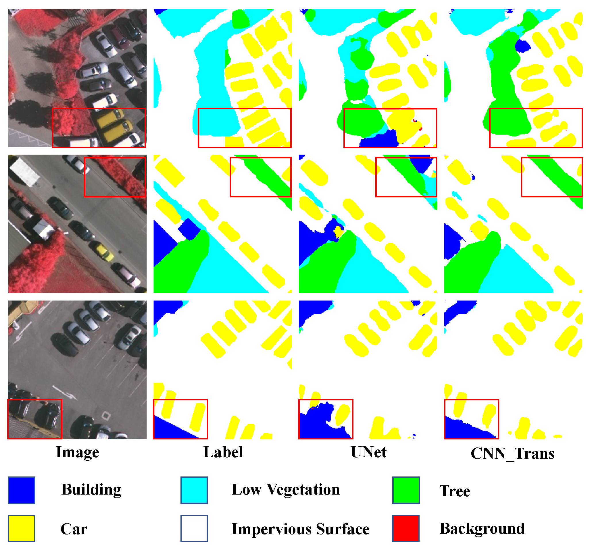
4.4.1. Validity of CNN and Transformer Hybrid Structure

As shown in

Table 1. Ablation results with different alterations on the Vaihingen dataset.

Method	Modules		IoU(%)					mIoU(%)	mF1(%)
	SCA_C	SCA_T	Building	Low Vegetation	Tree	Car	Impervious Surface
Baseline UNet			80.13	58.06	65.40	48.57	75.07	65.45	78.53
CNN_Trans			80.37	60.71	67.76	49.24	75.66	66.75	79.52
CNN_Trans+SCA_C	√		80.19	61.30	66.69	54.72	75.88	67.76	80.41
CNN_Trans+SCA_T		√	79.32	61.74	66.90	55.27	75.30	67.71	80.41
CNN_Trans+SCA_C+SCA_T	√	√	81.29	60.97	68.04	56.34	76.02	68.53	80.97

, we find that after applying the hybrid structure of a CNN and s Transformer, the model’s accuracy improves compared with the original UNet model. Furthermore, we find that the IoU of each category is dramatically improved, especially in the ’Low Vegetation’ category, which is enhanced by 2.65% and in the ’Tree’ category, enchanced by 2.36%; the final MIoU of the model increases by 1.30%. As shown in Figure 6, CNN_Trans exhibits significant performance in the segmentation of car targets while possessing the capability to extract global contextual information that UNet lacks. The results indicate that the Transformer effectively integrates the fine-grained texture information extracted by a CNN, thereby improving the recognition ability of small objects while maintaining the recognition ability for large objects.

4.4.2. Validity of SCA_C

The results in Table 1 demonstrate that our proposed SCA_C improves segmentation performance by 1.01% in mIoU and 0.89% in mF1. Specifically, after incorporating SCA_C into CNN_Trans, the model shows significant improvements in the segmentation accuracy of the ’Car’ class, with an increase of 5.48% in IoU and a 0.59% increase in IoU for the ’Low Vegetation’ class. To better observe the segmentation results, Figure 7 shows the comparison results of different models. In the boundary area, CNN_Trans usually cannot distinguish the boundary well because of the lack of spatial information. However, the SCA_C can effectively alleviate this problem. In the first row, due to some noise interference, CNN_Trans cannot identify the boundary and the corresponding object, but after the introduction of SCA_C, CNN_Trans can distinguish well. Through the above analysis, when using SCA_C to extract features, the segmentation accuracy of small targets and edge areas is effectively improved.

4.4.3. Validity of SCA_T

Table 1 shows that the accuracy of results increases by 0.96% in mIoU and 0.89% in mF1 when SCA_T is introduced in CNN_Trans. The utilization of SCA_T in the model leads to an improvement in the IoU of the ‘Low Vegetation’ category by 1.03% and a significant increase of 6.03% in the IoU of the ‘Car’ category, demonstrating the model’s powerful segmentation ability for small targets. Figure 8 depicts the specific situations where the model successfully identifies the targets in some blurred areas, particularly boundary regions. The model effectively identifies the car in the first and third rows even when other classes surround it. In the second row, the model can accurately identify the target and surrounding interference information due to the ability to extract global information brought about by SCA_T. The previous experimental results demonstrate the efficacy of SCA_T in facilitating both international and small target recognition.

As shown in Table 1, when we apply both SCA_T and SCA_C to CNN_Trans, the experimental results increase mIoU by 1.78% and mF1 by 1.45%. Compared with the UNet, our model improved by 3.08%mIoU and 2.44%mF1. The final experimental results demonstrate the effectiveness of our proposed two modules, which can improve the model’s performance in each category due to its strong ability to extract spatial and channel information.

4.5. Comparing the Segmentation Results of Different Models

In this study, we conduct a comprehensive comparison between our proposed CTFuse model and various existing models, including DeepLabv3, FCN, MANet, PSPNet, Res_UNet, UNet, Swin_UNet, ST_UNet, and Trans_UNet. The first six models are CNN-based, while Swin_UNet is entirely Transformer-based. ST_UNet adopts a parallel hybrid architecture of a CNN and a Transformer, whereas Trans_UNet follows a hybrid serial structure of a CNN and a Transformer. Notably, our CTFuse model also adopts a hybrid structure of a CNN and a Transformer. Distinct spatial and channel attention modules are integrated into the CNN and Transformer components to enhance feature extraction capability. For fairness, all comparison models undergo training solely on our designated training set and are evaluated on the test set without pre-training on other datasets. Throughout the experiments conducted on the Vaihingen and Potsdam datasets, CTFuse maintains consistency with the abovementioned models during both the training and testing phases.

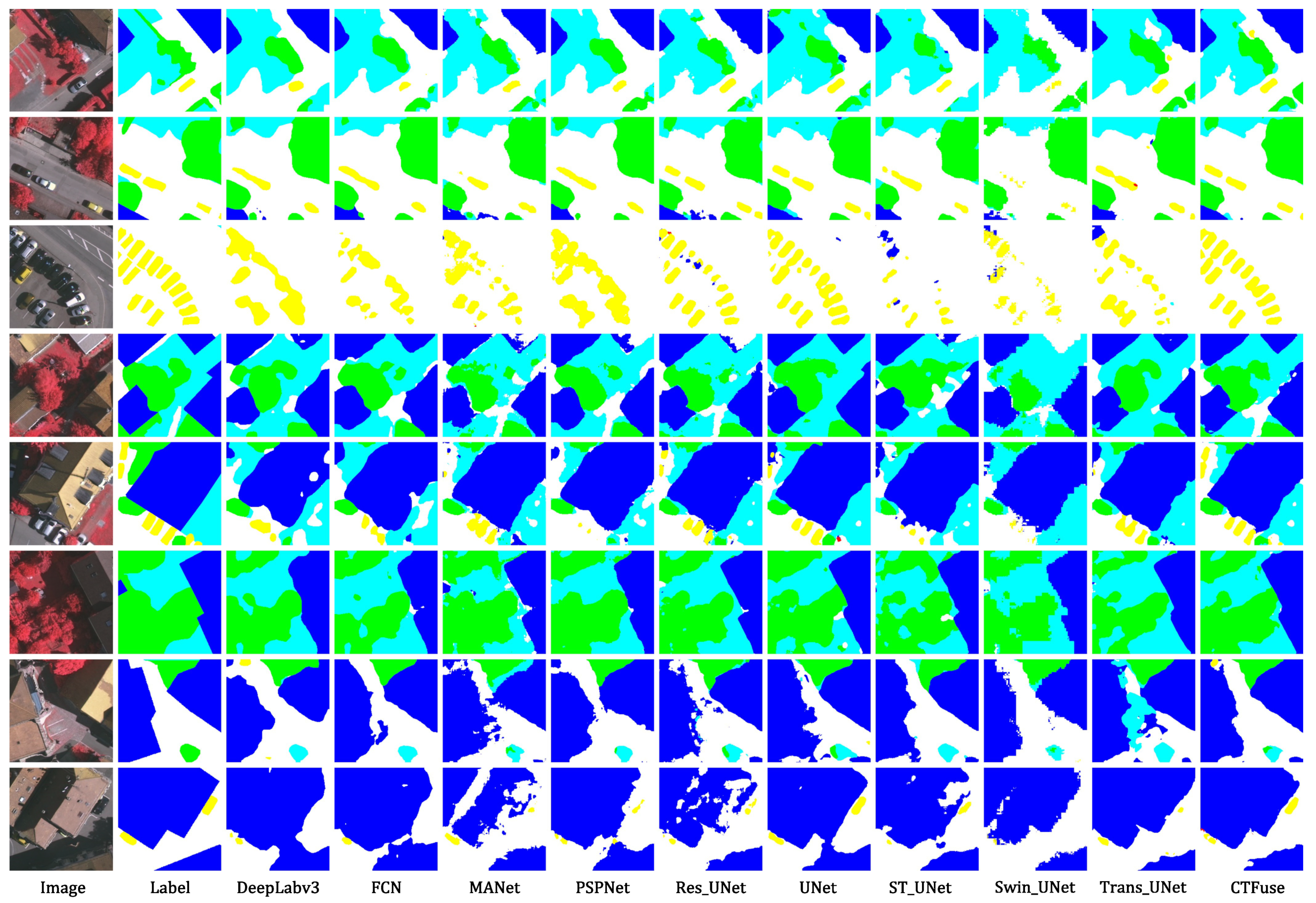
4.5.1. Experiments on the Vaihingen Dataset

Table 2. Comparing the results of different models on the Vaihingen dataset.

Method	Building		Low Vegetation		Tree		Car		Impervious Surface		mIoU (%)	mF1 (%)
	IoU	F1	IoU	F1	IoU	F1	IoU	F1	IoU	F1
DeepLabv3 [28]	74.28	85.24	56.86	72.50	64.54	78.45	27.81	43.52	70.75	82.87	58.85	72.52
FCN [24]	74.96	85.69	57.66	73.14	65.43	79.10	26.22	41.55	70.72	82.85	59.00	72.47
MANet [42]	72.96	84.37	55.52	71.40	63.89	77.96	27.90	43.63	81.94	76.29	57.93	70.73
PSPNet [29]	74.13	85.14	57.87	73.32	66.24	79.70	30.46	46.69	70.83	82.92	59.91	73.55
Res_UNet [40]	75.80	86.24	57.83	73.28	64.90	78.72	46.87	63.82	72.60	84.12	63.60	77.24
Unet [26]	80.13	88.97	58.06	73.47	65.40	79.08	48.57	65.38	75.07	85.76	65.45	78.53
ST_UNet [36]	74.29	85.25	52.53	68.88	57.72	73.19	22.17	36.29	69.73	82.16	55.29	69.15
Swin_UNet [46]	70.37	82.61	54.15	70.26	61.97	76.52	14.55	25.41	68.19	81.09	53.85	68.18
Trans_UNet [35]	74.75	85.55	56.17	71.94	62.87	77.20	34.71	51.53	71.19	83.17	59.94	73.88
CTFuse	$\mathbf{81}.\mathbf{29}$	$\mathbf{89}.\mathbf{68}$	$\mathbf{60}.\mathbf{97}$	$\mathbf{75}.\mathbf{75}$	$\mathbf{68}.\mathbf{04}$	$\mathbf{80}.\mathbf{98}$	$\mathbf{56}.\mathbf{34}$	$\mathbf{72}.\mathbf{07}$	$\mathbf{76}.\mathbf{02}$	$\mathbf{86}.\mathbf{37}$	$\mathbf{68}.\mathbf{53}$	$\mathbf{80}.\mathbf{97}$

shows the results of each model used in our experiments. As illustrated in Table 2, the CTFuse model achieves the best accuracy on the Vaihingen dataset and outperforms the comparison models regarding IoU per category, mIoU, and mF1. Deeplabv3 introduces the Atrous convolution and ASPP to expand the receptive field based on FCN, thereby improving the model’s ability to extract global context information. Ultimately, the FCN and Deeplabv3 achieved an mIoU of 59.00% and 58.85%, respectively. MANet uses kernel attention with linear complexity in the model, and we found that when the training set is small, its accuracy is low. PSPNet uses the Pyramid Pooling Module to combine spatial details of various sizes by pooling the original feature map to obtain different scales. As a result, PSPNet achieves 59.91% mIoU and 73.55% mF1. Res_UNet and UNet use the skip connection structure, while Res_UNet uses ResNet’s residual connection, Res_UNet, and UNet obtain 63.60% and 65.45% MIoU, respectively. Among the other models for comparison, the remaining three models are based on Transformers. Although Swin_UNet is composed of a Swin Transformer and has powerful global modeling capabilities, it does not show competitiveness in RS images. Similarly, when the training set is small, ST_UNet and Trans_UNet cannot offer a good result due to continuous downsampling and many Transformer parameters. In contrast, our proposed CTFuse model can achieve outstanding performance due to its powerful multi-scale spatial and channel feature extraction capabilities. Ultimately, the proposed CTFuse model gained 68.53% mIoU and 80.97% mF1, which is 3.08% mIoU and 2.44% mF1 higher than the results of the second-best UNet model.

We visualize the predicted segmentation results of each model on the Vaihingen dataset in Figure 9. Recognizing ‘Car’ is challenging when the ‘Car’ is in the shadows or when many ‘Car’ objects are close together. Some models recognize the car as part of ‘Low Vegetation’ or part of ‘Impervious Surface’ because ‘Car’ is usually surrounded by ‘Impervious Surface’ and ‘Low Vegetation’. Compared with other methods, our CTFuse has advantages in small target recognition. CTFuse can draw relatively accurate inferences by combining spatial and channel information for some difficult-to-distinguish features and fuzzy boundary information. In the first three rows in Figure 9, our model has an advantage in the category recognition of ‘Car’. The next five rows show that CTFuse has a strong performance in ‘Building’ and ‘Impervious Surface’, reflecting the model’s ability to integrate global context and local detail information.

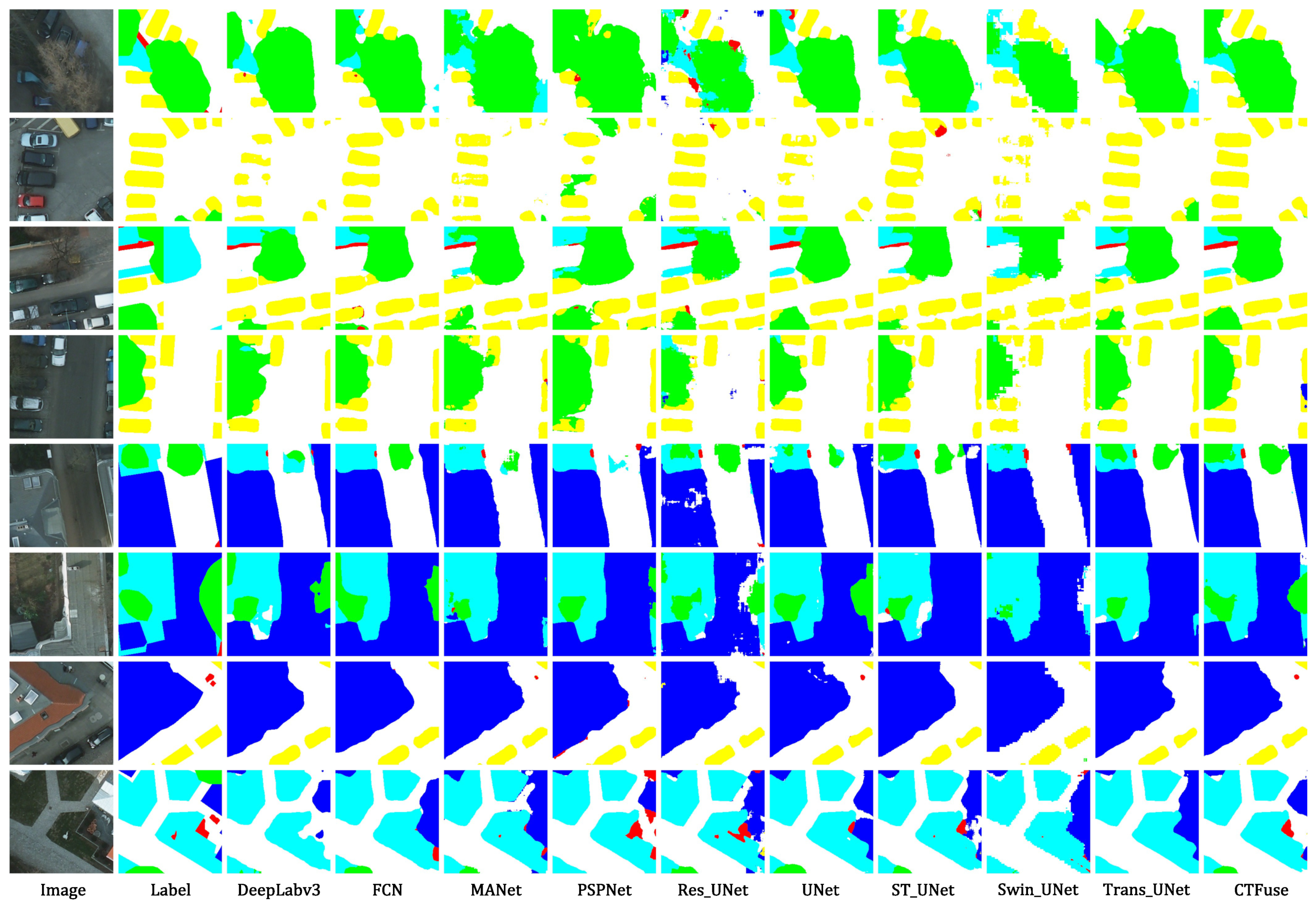
4.5.2. Experiments on the Potsdam Dataset

Table 3. Comparing the results of different models on the Potsdam dataset.

Method	Building		Low Vegetation		Tree		Car		Impervious Surface		mIoU (%)	mF1 (%)
	IoU	F1	IoU	F1	IoU	F1	IoU	F1	IoU	F1
DeepLabv3 [28]	81.71	89.93	60.77	75.60	55.71	71.56	68.00	80.95	74.49	85.38	68.14	80.68
FCN [24]	79.72	88.72	62.72	77.09	61.11	75.86	69.60	82.08	74.81	85.59	69.59	81.87
MANet [42]	78.07	87.68	61.13	75.88	56.97	72.59	67.67	80.72	72.89	84.32	67.35	80.24
PSPNet [29]	77.84	87.54	61.72	76.33	56.57	72.26	67.16	80.36	73.40	84.66	67.34	80.23
Res_UNet [40]	78.11	87.71	63.09	77.37	60.06	75.05	71.18	83.16	72.83	84.28	69.05	81.51
UNet [26]	81.77	89.97	64.34	78.30	61.70	76.32	72.39	83.98	75.22	85.86	71.08	82.89
ST_UNet [36]	82.20	90.23	62.45	76.88	58.62	73.91	67.90	80.88	73.32	84.60	68.90	81.30
Swin_UNet [46]	79.21	88.40	60.87	75.68	54.64	70.67	61.87	76.44	72.34	83.95	65.78	79.03
Trans_UNet [35]	81.95	90.08	62.37	76.83	58.09	73.49	67.17	80.36	74.11	85.13	68.74	81.18
CTFuse	$\mathbf{83}.\mathbf{13}$	$\mathbf{90}.\mathbf{79}$	$\mathbf{65}.\mathbf{07}$	$\mathbf{78}.\mathbf{84}$	$\mathbf{63}.\mathbf{93}$	$\mathbf{78}.\mathbf{00}$	$\mathbf{74}.\mathbf{12}$	$\mathbf{85}.\mathbf{13}$	$\mathbf{76}.\mathbf{04}$	$\mathbf{86}.\mathbf{39}$	$\mathbf{72}.\mathbf{46}$	$\mathbf{83}.\mathbf{83}$

illustrates the results of each segmentation model on the Potsdam dataset, where the CTFuse model obtains 72.46% mIoU and 83.83% mF1, which surpasses other models in the experiment. From Table 3, we can see that the accuracy of all models improved. Compared with the Vaihingen dataset, the Potsdam dataset has more data, and the ground sampling distance (GSD) is also greater. Hence, its segmentation requires less global information but more efficient feature extraction capabilities for local detail information, especially after dividing the picture into $256\times 256$. Therefore, the model must maintain a higher resolution in this scenario to obtain a better segmentation effect. The impact of Swin_UNet in this scene is not ideal because the downsampling ratio is too high, resulting in too much detailed information loss and affecting the segmentation results. ST_UNet, Trans_UNet, and Res_UNet used ResNet as the backbone in the early downsampling stage, so they obtained an approximate accuracy rate. UNet achieved 71.08% mIoU and 82.89% mF1 because it always maintains high-resolution feature maps. Compared with the abovementioned models, CTFuse achieves the highest segmentation accuracy due to its powerful ability to extract spatial and channel feature information.

Figure 10 demonstrates the segmentation results of all models used in our experiments. Models usually cannot extract enough information in low-brightness regions of the image, making objects in these regions challenging to recognize. In the first and fourth lines, we can see that when ‘Tree’ and ‘Car’ are mixed, it is difficult to separate the corresponding targets accurately. In this case, the CTFuse model can accurately identify dense and small-scale ground targets through its powerful ability to extract spatial and channel information. In the fifth to ninth lines, we can find that CTFuse also has a good effect on the recognition of large targets such as ‘Low Vegetation’ and ‘Building’, which reflects the model’s ability to extract global context information. At the same time, due to the limitation of the image, when the object is located in the edge area of the image, it is difficult to identify the target, and greater ability to extract detailed information is required.

4.5.3. Performance Analysis

To comprehensively compare the models, we show the computational speed and parameter amount of all the models used in our experiments in

Table 4. Comparing the results of different models on the Vaihingen dataset.

Method	Parameters (MB)	Speed (FPS)	Vaihingen (mIoU)	Potsdam (mIoU)
DeepLabv3 [28]	39.64	40.16	58.85	68.14
FCN [24]	32.95	47.95	59.00	69.59
MANet [42]	35.86	43.92	57.93	67.35
PSPNet [29]	65.58	5.50	59.91	67.34
Res_Unet [40]	13.04	53.82	63.60	69.05
Unet [26]	17.27	87.06	65.45	71.08
ST_Unet [36]	168.79	13.61	55.29	68.90
Swin_Unet [46]	27.18	60.19	53.85	65.78
Trans_Unet [35]	105.32	34.42	59.94	68.74
CTFuse	41.46	34.56	68.53	72.46

. Among them, ‘Speed’ represents the number of images that the model can process per second, and ‘Parameters’ means the memory resources required by the computer, and their units are ‘FPS’ and ‘MB’. The model using a Transformer usually has more parameters and a lower speed. Since we use MSCAN in the convolution part, relatively fast speed and small parameter amounts are obtained. The calculation speed of CTFuse is 34.56 FPS, and the parameter amount is 41.46 MB. Compared with convolution-based models, the speed of our CTFuse is still relatively slow, but it is still a valuable exploration for the combination of Transformer and CNN.

4.6. Visualization Analysis

To further elucidate the feature information that the CTFuse model focuses on in RS images, we employed the Grad-CAM [59] method to visualize the weights of the last convolutional layer in CTFuse. As depicted in Figure 11, Grad-CAM leverages the output feature map of a specific convolutional layer and the gradient information of the last fully connected layer to compute the significance of each position in the feature map for the classification result. The class-discriminative localization map $L_{Grad-CAM}^c\in {\mathbb{R}}^{H\times W}$ of class c is represented as follows:

$$L_{Grad-CAM}^c=ReLU\left({\sum }_k^{}{w}_k^c{A}^k\right),$$

(22)

$$w_k^c=\frac{1}{Z}{\sum }_i^{}{\sum }_j^{}\frac{\partial y^c}{\partial A_{ij}^k},$$

(23)

where k is the kth channel of feature map A. Z represents the product of width W and height H of the feature map. $A_{ij}^k$ represents the gradient value of backpropagation, and $y^c$ denotes the predicted score of class c. Specifically, it weights each position in the feature map according to the product of the gradient of the class score concerning the feature map and the feature map itself. Summing up these weighted activations generates an activation map, which is then passed through a ReLU activation function to obtain a class activation map. Finally, this class activation map is bilinearly upsampled to the size of the input image and visualized as a heatmap.

As shown in Figure 12, to better explore the areas of interest of the model, we visualize the Grad-CAM of different targets in the Vaihingen dataset. Highlighted areas in the image (red) indicate areas where the model pays attention to a particular class. In contrast, dark areas in the image indicate areas where the model pays less attention. For the three categories of ‘Building’, ‘Low Vegetation’, and ‘Impervious Surface’, which usually have large areas, the model accurately identifies the corresponding targets, demonstrating the ability of the model to obtain global context information effectively. When detecting ‘Low Vegetation’ and ‘Impervious Surface’, ‘Building’ has significant interference with them. Because the images taken by satellites do not have height information, the details of the three categories are relatively consistent. At the same time, the model can still recognize relatively small targets such as ‘Car’ and ‘Tree’ very well, demonstrating the model’s ability to extract local detail information. Therefore, the CTFuse model can effectively segment RS images.

4.7. Confusion Matrix

Figure 13 demonstrates the resulting confusion matrix after testing on the Vaihingen and Potsdom datasets. The proportion of accurately predicted image classes to the total predicted classes is represented by the image patch’s value at the confusion matrix’s main diagonal position. Darker image patches represent higher classification accuracy of the model, and brighter image patches represent lower classification accuracy. ‘Tree’ and ‘Low Vegetation’ are easily misclassified in the Vaihingen and Potsdom datasets since they are usually similar. ‘Car’ is easily misclassified as ‘Impervious Surface’ in Vaihingen, while it is relatively less in the Potsdom dataset because its ground sampling distance (GSD) is larger.

5. Conclusions

This research paper introduces a novel framework for semantic segmentation of RS images, denoted as CTFuse. This framework adopts a hybrid structure that combines the advantages of Transformers and a multi-scale convolutional attention network. By integrating CNN and Transformers, our approach effectively captures local and global information from RS images. Spatial and channel information plays a pivotal role in RS image segmentation, so we propose spatial and channel attention modules for both the CNN and Transformer components. These attention modules enhance the model’s capability to extract global context information and local detail information, contributing to improved segmentation performance.

Through comprehensive benchmark experiments and ablation studies conducted on the ISPRS Vaihingen and Potsdam datasets, we demonstrate the effectiveness and efficiency of the proposed CTFuse method in RS image segmentation, outperforming other models employed in the experiments. However, we acknowledge certain limitations in our current model, particularly in terms of unsmooth boundaries and shape discrepancies. As part of our future research direction, we aim to explore and refine our approach to achieve higher accuracy and efficiency in the RS image segmentation task.

References

1. Zhang, J.; Feng, L.; Yao, F. Improved maize cultivated area estimation over a large scale combining modis–evi time series data and crop phenological information. ISPRS J. Photogramm. Remote Sens. 2014, 94, 102–113. [Google Scholar] [CrossRef]
2. Zhang, C.; Harrison, P.A.; Pan, X.; Li, H.; Sargent, I.; Atkinson, P.M. Scale sequence joint deep learning (ss-jdl) for land use and land cover classification. Remote Sens. Environ. 2020, 237, 111593. [Google Scholar] [CrossRef]
3. Sahar, L.; Muthukumar, S.; French, S.P. Using aerial imagery and gis in automated building footprint extraction and shape recognition for earthquake risk assessment of urban inventories. IEEE Trans. Geosci. Remote Sens. 2010, 48, 3511–3520. [Google Scholar] [CrossRef]
4. Zhang, C.; Sargent, I.; Pan, X.; Li, H.; Gardiner, A.; Hare, J.; Atkinson, P.M. Joint deep learning for land cover and land use classification. Remote Sens. Environ. 2019, 221, 173–187. [Google Scholar] [CrossRef]
5. Fu, Y.; Zhao, C.; Wang, J.; Jia, X.; Yang, G.; Song, X.; Feng, H. An improved combination of spectral and spatial features for vegetation classification in hyperspectral images. Remote Sens. 2017, 9, 261. [Google Scholar] [CrossRef]
6. Aslam, B.; Maqsoom, A.; Khalil, U.; Ghorbanzadeh, O.; Blaschke, T.; Farooq, D.; Tufail, R.F.; Suhail, S.A.; Ghamisi, P. Evaluation of different landslide susceptibility models for a local scale in the chitral district, northern pakistan. Sensors 2022, 22, 3107. [Google Scholar] [CrossRef]
7. Tatsumi, K.; Yamashiki, Y.; Torres, M.A.C.; Taipe, C.L.R. Crop classification of upland fields using random forest of time-series landsat 7 etm+ data. Comput. Electron. Agric. 2015, 115, 171–179. [Google Scholar] [CrossRef]
8. Pal, M. Random forest classifier for remote sensing classification. Int. J. Remote Sens. 2005, 26, 217–222. [Google Scholar] [CrossRef]
9. Belgiu, M.; Drăguţ, L. Random forest in remote sensing: A review of applications and future directions. ISPRS J. Photogramm. Remote Sens. 2016, 114, 24–31. [Google Scholar] [CrossRef]
10. Cheng, Q.; Varshney, P.K.; Arora, M.K. Logistic regression for feature selection and soft classification of remote sensing data. IEEE Geosci. Remote Sens. Lett. 2006, 3, 491–494. [Google Scholar] [CrossRef]
11. Lee, S. Application of logistic regression model and its validation for landslide susceptibility mapping using gis and remote sensing data. Int. J. Remote Sens. 2005, 26, 1477–1491. [Google Scholar] [CrossRef]
12. Mas, J.F.; Flores, J.J. The application of artificial neural networks to the analysis of remotely sensed data. Int. J. Remote Sens. 2008, 29, 617–663. [Google Scholar] [CrossRef]
13. Gopal, S.; Woodcock, C. Remote sensing of forest change using artificial neural networks. IEEE Trans. Geosci. Remote Sens. 1996, 34, 398–404. [Google Scholar] [CrossRef]
14. Chebud, Y.; Naja, G.M.; Rivero, R.G.; Melesse, A.M. Water quality monitoring using remote sensing and an artificial neural network. Water Air Soil Pollut. 2012, 223, 4875–4887. [Google Scholar] [CrossRef]
15. Cheng, G.; Yang, C.; Yao, X.; Guo, L.; Han, J. When deep learning meets metric learning: Remote sensing image scene classification via learning discriminative cnns. IEEE Trans. Geosci. Remote Sens. 2018, 56, 2811–2821. [Google Scholar] [CrossRef]
16. Zhu, X.X.; Tuia, D.; Mou, L.; Xia, G.-S.; Zhang, L.; Xu, F.; Fraundorfer, F. Deep learning in remote sensing: A comprehensive review and list of resources. IEEE Geosci. Remote Sens. Mag. 2017, 5, 8–36. [Google Scholar] [CrossRef]
17. Shen, C.; Nguyen, D.; Zhou, Z.; Jiang, S.B.; Dong, B.; Jia, X. An introduction to deep learning in medical physics: Advantages, potential, and challenges. Phys. Med. Biol. 2020, 65, 05TR01. [Google Scholar] [CrossRef]
18. Hu, A.; Wu, L.; Chen, S.; Xu, Y.; Wang, H.; Xie, Z. Boundary shape-preserving model for building mapping from high-resolution remote sensing images. IEEE Trans. Geosci. Remote Sens. 2023, 61, 5610217. [Google Scholar] [CrossRef]
19. Hua, Y.; Mou, L.; Jin, P.; Zhu, X.X. Multiscene: A large-scale dataset and benchmark for multiscene recognition in single aerial images. IEEE Trans. Geosci. Remote Sens. 2021, 60, 1–13. [Google Scholar] [CrossRef]
20. Sun, J.; Yang, S.; Gao, X.; Ou, D.; Tian, Z.; Wu, J.; Wang, M. Masa-segnet: A semantic segmentation network for polsar images. Remote Sens. 2023, 15, 3662. [Google Scholar] [CrossRef]
21. Grinias, I.; Panagiotakis, C.; Tziritas, G. Mrf-based segmentation and unsupervised classification for building and road detection in peri-urban areas of high-resolution satellite images. ISPRS J. Photogramm. Remote. Sens. 2016, 122, 145–166. [Google Scholar] [CrossRef]
22. Benedek, C.; Descombes, X.; Zerubia, J. Building development monitoring in multitemporal remotely sensed image pairs with stochastic birth-death dynamics. IEEE Trans. Pattern Anal. Mach. Intell. 2011, 34, 33–50. [Google Scholar] [CrossRef] [PubMed]
23. Yi, Y.; Zhang, Z.; Zhang, W.; Zhang, C.; Li, W.; Zhao, T. Semantic segmentation of urban buildings from vhr remote sensing imagery using a deep convolutional neural network. Remote Sens. 2019, 11, 1774. [Google Scholar] [CrossRef]
24. Long, J.; Shelhamer, E.; Darrell, T. Fully convolutional networks for semantic segmentation. In Proceedings of the IEEE Conference on Computer Vision and Pattern Recognition 2015, Boston, MA, USA, 7–12 June 2015; pp. 3431–3440. [Google Scholar]
25. Qin, Y.; Kamnitsas, K.; Ancha, S.; Nanavati, J.; Cottrell, G.; Criminisi, A.; Nori, A. Autofocus layer for semantic segmentation. In Proceedings of the Medical Image Computing and Computer Assisted Intervention–MICCAI 2018: 21st International Conference, Granada, Spain, 16–20 September 2018; Proceedings, Part III 11. Springer: Berlin/Heidelberg, Germany, 2018; pp. 603–611. [Google Scholar]
26. Ronneberger, O.; Fischer, P.; Brox, T. U-net: Convolutional networks for biomedical image segmentation. In Proceedings of the Medical Image Computing and Computer-Assisted Intervention–MICCAI 2015: 18th International Conference, Munich, Germany, 5–9 October 2015; Proceedings, Part III 18. Springer: Berlin/Heidelberg, Germany, 2015; pp. 234–241. [Google Scholar]
27. Sinha, A.; Dolz, J. Multi-scale self-guided attention for medical image segmentation. IEEE J. Biomed. Health Inform. 2020, 25, 121–130. [Google Scholar] [CrossRef]
28. Chen, L.-C.; Papandreou, G.; Schroff, F.; Adam, H. Rethinking atrous convolution for semantic image segmentation. arXiv 2017, arXiv:1706.05587. [Google Scholar]
29. Zhao, H.; Shi, J.; Qi, X.; Wang, X.; Jia, J. Pyramid scene parsing network. In Proceedings of the IEEE Conference on Computer Vision and Pattern Recognition 2017, Honolulu, HI, USA, 21–26 July 2017; pp. 2881–2890. [Google Scholar]
30. Dosovitskiy, A.; Beyer, L.; Kolesnikov, A.; Weissenborn, D.; Zhai, X.; Unterthiner, T.; Dehghani, M.; Minderer, M.; Heigold, G.; Gelly, S. An image is worth 16x16 words: Transformers for image recognition at scale. arXiv 2020, arXiv:2010.11929. [Google Scholar]
31. Carion, N.; Massa, F.; Synnaeve, G.; Usunier, N.; Kirillov, A.; Zagoruyko, S. End-to-end object detection with Transformers. In Proceedings of the Computer Vision–ECCV 2020: 16th European Conference, Glasgow, UK, 23–28 August 2020; Proceedings, Part I 16. Springer: Berlin/Heidelberg, Germany, 2020; pp. 213–229. [Google Scholar]
32. Zheng, S.; Lu, J.; Zhao, H.; Zhu, X.; Luo, Z.; Wang, Y.; Fu, Y.; Feng, J.; Xiang, T.; Torr, P.H. Rethinking semantic segmentation from a sequence-to-sequence perspective with Transformers. In Proceedings of the IEEE/CVF Conference on Computer Vision and Pattern Recognition 2021, Nashville, TN, USA, 20–25 June 2021; pp. 6881–6890. [Google Scholar]
33. Guo, M.-H.; Lu, C.-Z.; Hou, Q.; Liu, Z.; Cheng, M.-M.; Hu, S.-M. Segnext: Rethinking convolutional attention design for semantic segmentation. arXiv 2022, arXiv:2209.08575. [Google Scholar]
34. Ioannou, Y.; Robertson, D.; Cipolla, R.; Criminisi, A. Deep roots: Improving cnn efficiency with hierarchical filter groups. In Proceedings of the IEEE Conference on Computer Vision and Pattern Recognition 2017, Honolulu, HI, USA, 21–26 July 2017; pp. 1231–1240. [Google Scholar]
35. Chen, J.; Lu, Y.; Yu, Q.; Luo, X.; Adeli, E.; Wang, Y.; Lu, L.; Yuille, A.L.; Zhou, Y. Transunet: Transformers make strong encoders for medical image segmentation. arXiv 2021, arXiv:2102.04306. [Google Scholar]
36. He, X.; Zhou, Y.; Zhao, J.; Zhang, D.; Yao, R.; Xue, Y. Swin transformer embedding unet for remote sensing image semantic segmentation. IEEE Trans. Geosci. Remote Sens. 2022, 60, 1–15. [Google Scholar] [CrossRef]
37. Song, P.; Li, J.; An, Z.; Fan, H.; Fan, L. Ctmfnet: Cnn and Transformer multi-scale fusion network of remote sensing urban scene imagery. IEEE Trans. Geosci. Remote Sens. 2022. [Google Scholar] [CrossRef]
38. Zhang, Y.; Lu, H.; Ma, G.; Zhao, H.; Xie, D.; Geng, S.; Tian, W.; Sian, K.T.C.L.K. Mu-net: Embedding mixformer into unet to extract water bodies from remote sensing images. Remote Sens. 2023, 15, 3559. [Google Scholar] [CrossRef]
39. Wang, D.; Chen, Y.; Naz, B.; Sun, L.; Li, B. Spatial-aware transformer (sat): Enhancing global modeling in transformer segmentation for remote sensing images. Remote Sens. 2023, 15, 3607. [Google Scholar] [CrossRef]
40. Zhang, Z.; Liu, Q.; Wang, Y. Road extraction by deep residual u-net. IEEE Geosci. Remote Sens. Lett. 2018, 15, 749–753. [Google Scholar] [CrossRef]
41. He, K.; Zhang, X.; Ren, S.; Sun, J. Deep residual learning for image recognition. In Proceedings of the IEEE Conference on Computer Vision and Pattern Recognition, Las Vegas, NV, USA, 26 June–1 July 2016; pp. 770–778. [Google Scholar]
42. Li, R.; Zheng, S.; Zhang, C.; Duan, C.; Su, J.; Wang, L.; Atkinson, P.M. Multiattention network for semantic segmentation of fine-resolution remote sensing images. IEEE Trans. Geosci. Remote Sens. 2021, 60, 1–13. [Google Scholar] [CrossRef]
43. Ashish, V. Attention is all you need. Adv. Neural Inf. Process. Syst. 2017, 30, I. [Google Scholar]
44. Xie, E.; Wang, W.; Yu, Z.; Anandkumar, A.; Alvarez, J.M.; Luo, P. Segformer: Simple and efficient design for semantic segmentation with Transformers. Adv. Neural Inf. Process. Syst. 2021, 34, 12077–12090. [Google Scholar]
45. Lin, T.; Wang, Y.; Liu, X.; Qiu, X. A survey of Transformers. AI Open 2022, 3, 111–132. [Google Scholar] [CrossRef]
46. Cao, H.; Wang, Y.; Chen, J.; Jiang, D.; Zhang, X.; Tian, Q.; Wang, M. Swin-unet: Unet-like pure Transformer for medical image segmentation. In Proceedings of the Computer Vision–ECCV 2022 Workshops, Tel Aviv, Israel, 23–27 October 2022; Proceedings, Part III. Springer: Berlin/Heidelberg, Germany, 2023; pp. 205–218. [Google Scholar]
47. Yu, C.; Wang, F.; Shao, Z.; Sun, T.; Wu, L.; Xu, Y. Dsformer: A double sampling transformer for multivariate time series long-term prediction. arXiv 2023, arXiv:2308.03274. [Google Scholar]
48. Zhang, W.; Huang, Z.; Luo, G.; Chen, T.; Wang, X.; Liu, W.; Yu, G.; Shen, C. Topformer: Token pyramid transformer for mobile semantic segmentation. In Proceedings of the IEEE/CVF Conference on Computer Vision and Pattern Recognition, New Orleans, LA, USA, 18–24 June 2022; pp. 12083–12093. [Google Scholar]
49. Ba, J.; Mnih, V.; Kavukcuoglu, K. Multiple object recognition with visual attention. arXiv 2014, arXiv:1412.7755. [Google Scholar]
50. Hu, J.; Shen, L.; Sun, G. Squeeze-and-excitation networks. In Proceedings of the IEEE Conference on Computer Vision and Pattern Recognition, Salt Lake City, UT, USA, 18–23 June 2018; pp. 7132–7141. [Google Scholar]
51. Dai, J.; Qi, H.; Xiong, Y.; Li, Y.; Zhang, G.; Hu, H.; Wei, Y. Deformable convolutional networks. In Proceedings of the IEEE International Conference on Computer Vision, Venice, Italy, 22–29 October 2017; pp. 764–773. [Google Scholar]
52. Woo, S.; Park, J.; Lee, J.-Y.; Kweon, I.S. Cbam: Convolutional block attention module. In Proceedings of the European Conference on Computer Vision (ECCV), Munich, Germany, 8–14 September 2018; pp. 3–19. [Google Scholar]
53. Fu, J.; Liu, J.; Tian, H.; Li, Y.; Bao, Y.; Fang, Z.; Lu, H. Dual attention network for scene segmentation. In Proceedings of the IEEE/CVF Conference on Computer Vision and Pattern Recognition, Long Beach, CA, USA, 15–20 June 2019; pp. 3146–3154. [Google Scholar]
54. ISPRS. Semantic Labeling Contest-Vaihingen (2018). Available online: https://www2.isprs.org/commissions/comm2/wg4/benchmark/2d-sem-label-vaihingen/ (accessed on 4 September 2021).
55. Gao, L.; Liu, H.; Yang, M.; Chen, L.; Wan, Y.; Xiao, Z.; Qian, Y. Stransfuse: Fusing swin Transformer and convolutional neural network for remote sensing image semantic segmentation. IEEE J. Sel. Top. Appl. Earth Obs. Remote Sens. 2021, 14, 10990–11003. [Google Scholar] [CrossRef]
56. Wang, L.; Li, R.; Zhang, C.; Fang, S.; Duan, C.; Meng, X.; Atkinson, P.M. Unetformer: A unet-like Transformer for efficient semantic segmentation of remote sensing urban scene imagery. ISPRS J. Photogramm. Remote Sens. 2022, 190, 196–214. [Google Scholar] [CrossRef]
57. ISPRS. Semantic Labeling Contest-Potsdam (2018). Available online: http://www2.isprs.org/commissions/comm3/wg4/2d-sem-label-potsdam.html (accessed on 4 September 2021).
58. Milletari, F.; Navab, N.; Ahmadi, S.-A. V-net: Fully convolutional neural networks for volumetric medical image segmentation. In Proceedings of the 2016 Fourth International Conference on 3D Vision (3DV), Stanford, CA, USA, 25–28 October 2016; pp. 565–571. [Google Scholar]
59. Selvaraju, R.R.; Cogswell, M.; Das, A.; Vedantam, R.; Parikh, D.; Batra, D. Grad-cam: Visual explanations from deep networks via gradient-based localization. In Proceedings of the IEEE International Conference on Computer Vision, Venice, Italy, 22–29 October 2017; pp. 618–626. [Google Scholar]
Figure 1. Illustration of local and global information.
Remotesensing 15 04455 g001
Figure 2. (a) A multi-scale convolutional attention (MSCA) module [33]. (b) MSCA with our proposed SCA_C block (SC_MSCAN). (c) The standard Transformer block [43]. (d) Transformer with the proposed SCA_T block (SC_Transformer).
Remotesensing 15 04455 g002
Figure 3. Architecture of our proposed CTFuse.
Remotesensing 15 04455 g003
Figure 4. Structure of SCA_C.
Remotesensing 15 04455 g004
Figure 5. Structure of SCA_T.
Remotesensing 15 04455 g005
Figure 6. Comparing the segmentation results of UNet and CNN_Trans.
Remotesensing 15 04455 g006
Figure 7. Comparing the segmentation results of UNet and CNN_Trans +SCA_C.
Remotesensing 15 04455 g007
Figure 8. Comparing the segmentation results of UNet and CNN_Trans +SCA_T.
Remotesensing 15 04455 g008
Figure 9. Comparing the segmentation results of different models on the Vaihingen dataset.
Remotesensing 15 04455 g009
Figure 10. Comparing the segmentation results of different models on the Potsdam dataset.
Remotesensing 15 04455 g010
Figure 11. Overview of the application of Grad-CAM visualization method.
Remotesensing 15 04455 g011
Figure 12. The Grad-CAM visualization of different classes of features.
Remotesensing 15 04455 g012
Figure 13. Confusion matrix of CTFuse model on the Vaihingen and Potsdom datasets.
Remotesensing 15 04455 g013