1. Introduction
Gravity data are crucial for studying the Earth’s gravity field and establishing the International Height Reference System (IHRS). Currently, global gravity field models (GGMs) are routinely used to provide long wavelength information for regional gravity field modeling. Apart from GGMs, terrestrial gravity data are the most widely used data type. However, in areas that are challenging to access (e.g., polar regions, mountains, forests, coastal areas, oceans) or in very large areas (e.g., >10,000 km
2), airborne gravity practically becomes the only option [
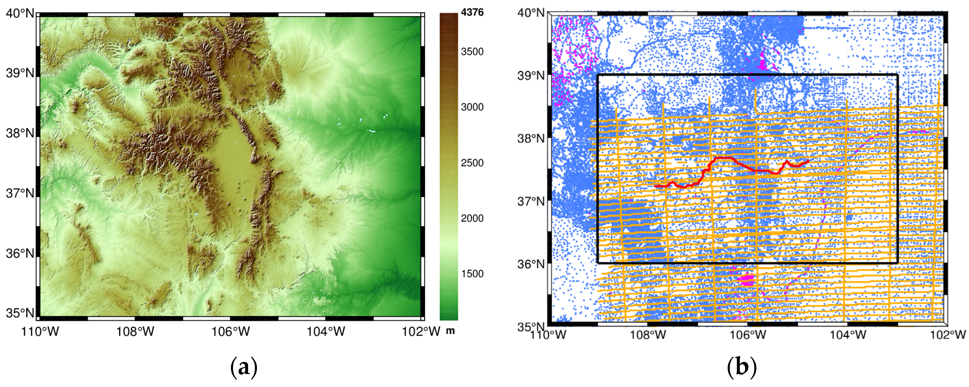
1]. In 2017, the Joint Working Group (JWG) 2.1.2 of the International Association of Geodesy (IAG) launched the Colorado geoid experiment (the 1 cm geoid experiment). The goal of this experiment is to assess the repeatability of gravity potential values as IHRS coordinates using different geoid modeling methods. In this context, the National Geodetic Survey (NGS) agreed to provide terrestrial gravity data, airborne gravity data, GPS/leveling data, and a digital terrain model for an area of approximately 500 km × 800 km in Colorado, which allowed the comparison of different methods for geoid computation using the same input dataset.
However, when using terrestrial and airborne gravity for local geoid refinement, there are several challenges that need to be addressed. First, terrestrial and airborne gravity data differ not only in spatial distribution and spectral content but also in their error characteristics. Therefore, a major challenge for geoid modeling is the proper combination of terrestrial and airborne gravity data. Second, both terrestrial and airborne gravity observations are unevenly distributed, leading to uncertainty in their spectral information. The spectral information of gravity data is closely related to their spatial resolution. However, determining the appropriate resolution of both terrestrial and airborne gravity data is difficult. The terrestrial gravity data resolution relies heavily on topographic heights, the distribution of which are usually extremely uneven, while the resolution of airborne gravity observations is influenced by factors such as the flight altitude, speed, and data correlation. All of these factors pose significant challenges in determining the optimal spectrum of gravity data. Third, for airborne gravity data, a downward continuation process is typically required [
2,
3,
4]. However, the downward continuation process is an unstable procedure that amplifies high-frequency noise, leading to a reduction in the quality of airborne data. Moreover, a series of filtering and estimation techniques are usually required for airborne gravity data, which further exacerbate the uncertainty of the spectral information for airborne gravity data. It has been observed that using gravity signals beyond their corresponding spherical harmonic (SH) degree can introduce modeling errors [
5]. Therefore, finding and modeling the useful information provided by gravity data has become a critical issue in local geoid enhancement [
6].
Several methods can be employed to refine the regional geoid model, such as the well-known least squared collocation (LSC) method [
7], least squares spectral combination method [
8,
9], and Slepian functions [
10]. In this study, we chose to use band-limited spherical radial basis functions (SRBFs) for local geoid refinement. The justifications for this choice are as follows. First, the band-limited SRBFs can be adjusted flexibly based on the spectral information of the gravity data, which allows for better adaptation to the spectral characteristics of the gravity data. Second, band-limited SRBFs can express almost all types of gravity data, which form the basis for combining multisource gravity data to build a high-resolution regional gravity field model. Third, the band-limited SRBF expression includes a continuation factor, allowing the establishment of observation equations directly at scattered points of observation without the need for gridding or downward continuation. This feature enables the assignment of observation errors to specific observables in space. Li utilized a set of band-limited SRBFs to model gravity data and demonstrated that the SRBF method could effectively recover the gravity field while exhibiting filtering properties due to its design in the frequency domain. Additionally, experiments have shown that SRBFs are computationally efficient and do not require a covariance model such as the LSC method, which is sometimes time-consuming [
11]. Other examples and explanations of SRBFs can also be found in [
12,
13,
14,
15,
16,
17,
18,
19,
20,
21] and the references therein.
In this study, our main focus is on refining the regional geoid model in Colorado using band-limited SRBFs. To determine the optimal spectral information of the gravity data, we propose a residual and a priori accuracy comparative analysis method. The organization of this work is as follows. In
Section 2, we present the fundamental concepts of SRBFs and the parameter estimation procedure. This includes the formulation of observation equations, estimation of unknown coefficients, and calculation of gravitational functionals. In
Section 3, we introduce the study area in Colorado and describe the available data. We also outline the procedure for data preprocessing. In
Section 4, we explain the computation procedure, which involves the RCR procedure, the residual and a priori accuracy comparative analysis method, and how we combine different datasets.
Section 5 presents our models as well as the validation of the results. Finally,
Section 6 provides the conclusions and presents potential future research directions.
2. Theory and Methods
A residual harmonic function
outside a sphere of radius
R can be written as a finite sum of band-limited SRBFs:
where
is the position vector of the observation point
P,
is the spherical longitude,
is the spherical latitude, and
, with
being the spherical height of
P above sphere
with radius
R.
are the position vectors of the SRBFs.
is the number of SRBFs,
is the residual disturbing potential, and
is the unknown coefficient.
is a band-limited SRBF, the specific expression for which is [
22]
where
is the kernel function that defines the spectral properties of the SRBFs,
is the mean radius of Earth,
is the Legendre polynomial of degree
, and
is the spherical distance between
and
.
and
are the minimum and maximum degrees of expansion, respectively. The SRBF in Equation (2) is band-limited since the kernel functions are zero for each degree beyond
or below
.
The general expression of Equation (2) needs to be adapted to describe different gravitational functionals. We use observations that are given in terms of gravity disturbances
, which can be expressed as the gradient of the disturbing potential
. In the spherical approximation, the magnitude of the gravity disturbance can be written as [
23]
From the SRBF expression for the disturbing potential (Equation (1)), the residual terrestrial gravity disturbances at the Earth’s surface and the residual airborne gravity disturbances at flight altitude can be written as
where
and
represent the position vectors of terrestrial and airborne gravity disturbances, respectively.
and
are the maximum degrees of expansion of the terrestrial and airborne gravity disturbances, respectively.
are the adapted SRBFs of
.
For terrestrial gravity observations, it is difficult to obtain a more appropriate expansion degree due to their uneven distribution. For airborne gravity data, however, due to their high altitudes and the low-pass filtering process, it is also not a simple task to determine optimal spectral information. In this study, we provide a way to determine the optimal degree of series expansion for gravity data (
and
), which will be introduced in
Section 4.2.
In Equation (4), terrestrial gravity disturbances and airborne gravity disturbances have the same SRBF coefficients
, and we can thus combine them to form the observation equations (Gauss–Markov model)
where
and
are the vectors of the terrestrial and airborne gravity disturbances, and
and
are the design matrices.
are the unknown SRBF coefficients, and
and
are the vectors of observation errors with expectation
and dispersion
.
is the variance-covariance matrix of the observed error and meets
;
and
are the observation weight matrices for group
.
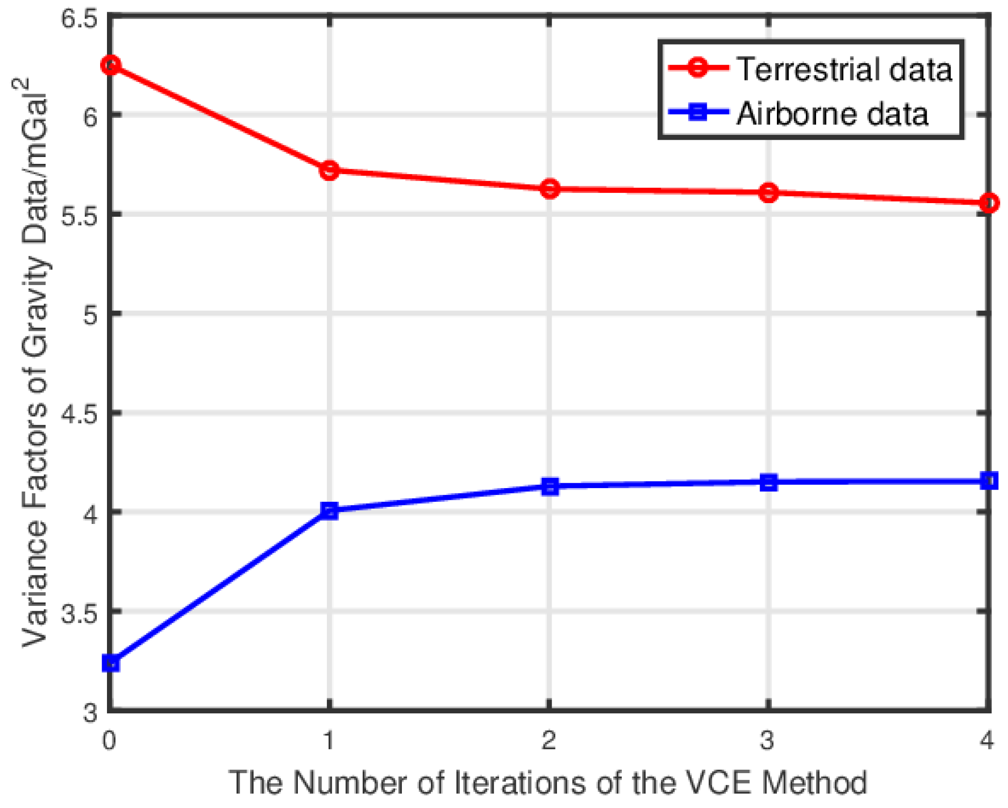
Usually, the normal equation matrix of Equation (5) is ill conditioned, and stabilization is needed to make the computation of a solution possible. Moreover, since the true accuracy of the two datasets is not exactly known, it is especially necessary to determine reasonable variance factors when building the gravity field model by combining terrestrial and airborne gravity data. All of these requirements can be met using the variance component estimation method (VCE) [
24]
where
and
are the variance factors of terrestrial and airborne gravity disturbances, respectively.
is the variance factor of unknown coefficients, which is also a regularization parameter, and
is the unit matrix. The variance factors are usually determined based on an iterative method. Specifically, the initial variance factors
,
, and
are first given, and then the initial SRBF coefficients are estimated with the least squares estimation method. Then, the residuals of the least square values of the observations are further obtained, and the new variance factors can be calculated by
where
and
are the residuals after the
th iteration,
are the variance factors of the
th group of observations after the
th iteration, and
is the variance factor of the unknown coefficients.
and
are redundant numbers, which can be expressed as
where
represents the number of gravity observations of group
,
is the number of coefficients of SRBFs,
is the design matrix at the
th iteration,
is the matrix of the normal equation at the
th iteration, and
is the total normal equation matrix at the
th iteration.
stands for trace operation. For the computation of the partial redundancies in Equations (9) and (10), the inverse matrix
of normal equations is needed. We use the stochastic trace estimation theorem proposed by Hutchinson [
25].
After the new variance factors are calculated, the next loop is entered until the convergence condition of the following equation is satisfied:
where
is the convergence threshold, and we set
in this study.
Applying the least squares method to Equation (6), the unknown coefficients are estimated as
Inserting the coefficients of Equation (12) back into Equation (1), we can obtain the residual disturbing potential .
The residual height anomaly is related to the residual disturbing potential
by
where
is the normal gravity defined at the telluroid and
is the residual height anomaly.
Then, during the recovery procedure, we add back the height anomaly component of the GGM and the topographic effects, and a full-wavelength height anomaly can be obtained.
Finally, the geoid undulation can be obtained by the following conversion:
where
is the orthometric height,
is the geoid undulation, and
is the simple Bouguer anomaly. Higher-order terms of the separation term [
26] are not considered here, to be consistent with previously published procedures.
4. Gravity Field Modeling
In gravity field modeling based on band-limited SRBFs, several parameters and procedures are considered.
① Geocentric gravitational constant (): 3.986 004 415 × .
② Average density of topographic masses (): 2670 .
③ Geoid computations are performed in the tidefree system. GRS80 is used as the reference ellipsoid, and the conventional constants are taken from Moritz (2000).
Apart from these fundamental parameters, four important factors that influence the performance of SRBFs are also accounted for, namely (1) the type of the SRBFs; (2) the location of the SRBFs; (3) the extensions of the observation area, computation area, and target area; and (4) the maximum and minimum expansion degree of the SRBFs. Considering these parameters and procedures helps to ensure an effective and accurate gravity field modeling process based on band-limited SRBFs. Next, we introduce the model configuration for gravity field modeling based on band-limited SRBFs.
4.1. Model Configuration
4.1.1. Types of SRBFs
There are many types of SRBFs that can be used for gravity field modeling, such as the Shannon functions, the Blackman functions, the Poisson functions, and the cubic polynomial functions. The Shannon function is a reproducing kernel of the space spanned by all solid spherical harmonics of degrees
[
45]. As a result, it does not smooth the gravity signal in this spectral band. However, other types of SRBFs (e.g., Blackman functions, Poisson functions, and cubic polynomial functions) with nonconstant kernel functions might smooth some gravity field harmonics. Although some harmonic properties still remain in the recovered signal, they might be significantly suppressed. Therefore, one has to be careful when interpreting results based on the SRBFs with smoothing kernel functions. Moreover, Bentel et al. studied the performance of different types of SRBFs, and the results show that the Shannon SRBFs lead to the same results as with spherical harmonics both in theory and in practice. Therefore, in this study, the Shannon kernel functions are used, the specific form of which is
4.1.2. The Location of the SRBFs
The location of the SRBFs depends on the type of grid. There are many types of grids that can be used for regional gravity field modeling, such as the Driscoll–Healy grid, the triangle vertex grid, and the Reuter grid [
46]. Eicker analyzed the advantages and disadvantages of different types of grids, and the results show that both the Reuter grids and the triangle vertex grids are suitable for gravity field modeling with SRBFs. Bentel et al. noted that different types of grids do not differ significantly, especially compared to the other three factors that influence the modeling results. In addition, the control parameter
of the Reuter grids is related to the maximum expansion degree of SRBFs, which also facilitates gravity field modeling. We set
, where
is the maximum degree of the series expansion of SRBFs.
4.1.3. The Extensions of the Target, Observation, and Computation Area
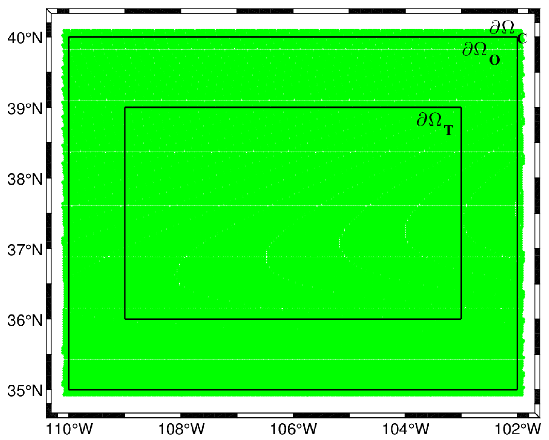
In regional gravity modeling, the extension of the target area
, the observation area
, and the computation area
needs to be defined carefully. At the edge of the observation area
, the unknown coefficients cannot be appropriately estimated, which provokes edge effects. In general, the target area
should be smaller than the observation area
, and the computation area
should be larger than the observation area
[
47]. Therefore, to minimize the edge effects in the computation,
should be satisfied. In addition, the margin size
needs to be defined between the three areas. In our case, the target area
is given to be between −109
and −103
and 36
and 39
. Therefore, the margin size
between
and
is fixed to 1
.
The determination of the margin size
between
and
follows the empirical formula described by Liu et al.:
where
is the maximum latitude value of the study area. In this study,
(see
Section 4.3). By substituting this value into formula (20), the value
follows.
Figure 4 visualizes the target area, the observation area, the computation area, and the margins.
4.1.4. Maximum and Minimum Expansion Degree of SRBFs
The maximum degree of expansion of SRBFs is usually determined by high-resolution gravity data, which can be determined by empirical rules [
48]
where Resol represents the resolution of the gravity data. In this study, the spatial resolution of terrestrial data is higher than that of airborne data. Therefore, the maximum expansion degree of the SRBFs is mainly determined by terrestrial data. Moreover, Liu et al. claimed that the average spatial interval of terrestrial gravity data is approximately 3.5 km, so they expanded the SRBFs to degree 5600. However, the maximum expansion degree determined by Liu et al. may be inappropriate, since Grigoriadis et al. stated that only approximately 50% of the cells in the
grid contained at least one value, which suggests that the data distribution may not be suitable to support such a high maximum degree of expansion. Therefore, we suggest expanding the SRBFs for terrestrial gravity data to a degree of less than 5400. However, determining the optimal spectral range for both terrestrial and airborne gravity data is difficult. To address this issue, we propose the residual and a priori accuracy comparative analysis method, which will be discussed in detail in
Section 4.2.
For the minimum degree of expansion, Bucha et al. noted that there is still useful gravity information below the cutoff degree of the GGM. They concluded that starting the series expansion of SRBFs at a lower degree, such as 0, can help to capture this useful part of the signal. This method has been commonly used in local gravity field modeling. However, it seems that this method is not always effective. In this study, since the contributions of XGM2016 up to degree 719 have been removed from the original signals, we set . By using this minimum degree starting from 720 instead of 0, we obtain better results, at least in the Colorado region of this study.
4.2. Residual and A Priori Accuracy Comparative Analysis Method
To efficiently use the gravity data for gravity field modeling, the residual and a priori accuracy comparative analysis method is proposed to determine the optimal expansion degree of the gravity data. The procedure is as follows.
Step 1: Within a large search interval, certain degrees with a large step size are selected as the maximum expansion degrees of the gravity data. Terrestrial-only and airborne-only SRBF models are then built using these maximum expansion degrees. Finally, the model with the smallest difference between the RMS value of the modeling residuals and the a priori accuracy of the gravity data is taken as the initial model, and its corresponding expansion degree is identified as the initial degree.
Step 2: A smaller range around the initial degree is defined with a smaller degree step size, and new SRBF models are constructed within this range. The differences between these models and the GSVS17 data are calculated to obtain the STD value for each model. Finally, the model that has the smallest STD value is determined, and the corresponding expansion degree is considered the optimal expansion degree of the gravity data.
It is important to note that Step 1 helps to reduce the calculation time and improve the efficiency. Due to the large amount of gravity data, calculating the STD value for the geoid height differences for each model would require significant computational time. By initially selecting a larger degree range, the computational effort is reduced. In Step 2, external data (GSVS17) are used to assess the quality of the SRBF model within a smaller range. This is because there is some uncertainty in the a priori accuracy of both terrestrial and airborne data. By incorporating external data within a smaller degree range, the computational effort is further reduced.
4.3. Gravity Field Modeling with SRBFs
We combine the terrestrial and airborne data using the Gauss–Markov model (Equation (5)). Saleh et al. studied the qualities of the terrestrial gravity database of NGS, and the results show that the accuracy of terrestrial data is approximately 2.2 mGal [
49]. Moreover, Varga et al. estimated the accuracy of terrestrial gravity data assuming that the errors are uncorrelated and obtained accuracy of 2.6 mGal. In addition, other scholars have estimated terrestrial gravity data at 1 mGal [
50] or 3 mGal [
51]. However, it seems that the accuracy of 1 mGal may be overstated, while the accuracy of 3 mGal may be understated. Therefore, we set the a priori accuracy of the terrestrial gravity data to 2.2 mGal, which is essentially consistent with the results of Saleh et al. Moreover, the a priori accuracy of the airborne gravity data is approximately 1.6–2 mGal [
52], and we take the median value of 1.8 mGal as its a priori accuracy.
The determination of the optimal expansion degree of terrestrial and airborne gravity data is conducted using the residual and a priori accuracy comparative analysis method.
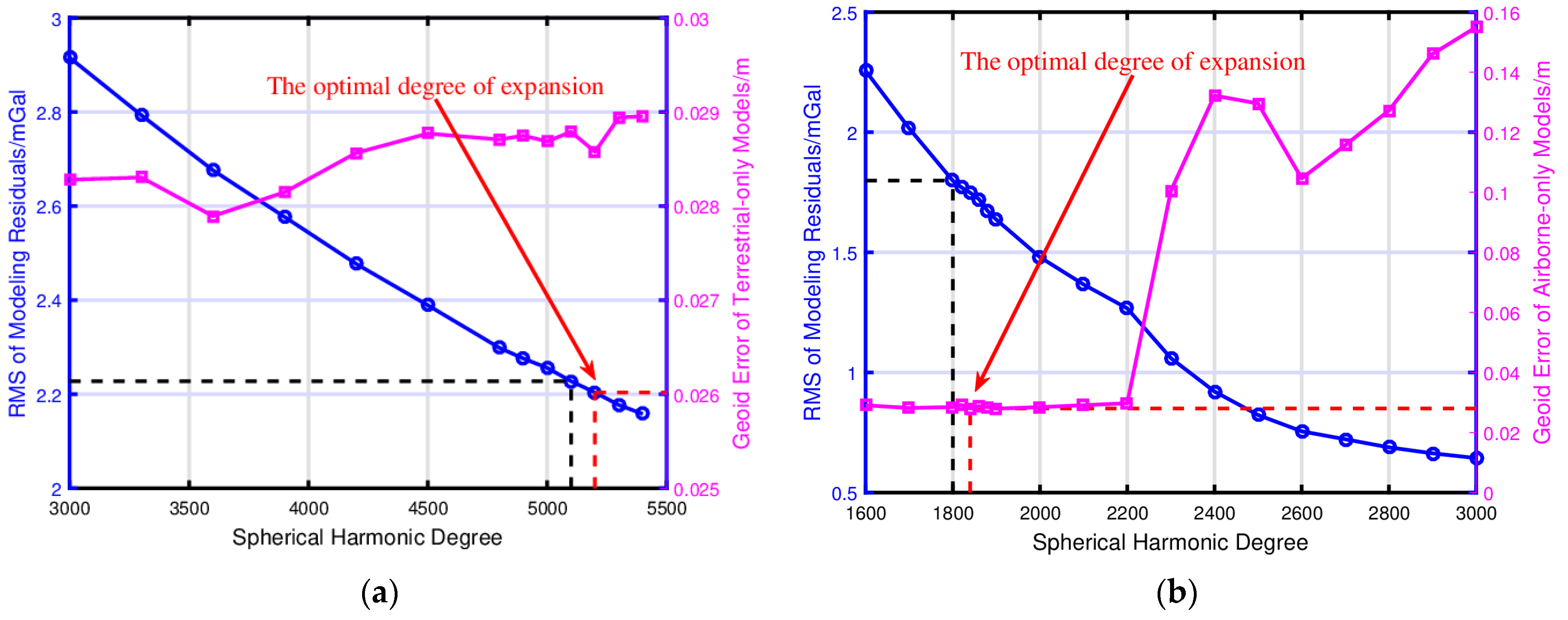
Figure 5 illustrates the procedure to determine the optimal expansion degree of the gravity data. To fully demonstrate the differences caused by the different expansion degrees of SRBFs, the STD values of the geoid height differences between each model and GSVS17 are also calculated.
Figure 5a shows that a search range of 3000 to 5400, with a step size of 300, is selected for the terrestrial gravity data in Step 1. For the airborne gravity data, a search range of 1600 to 3000, with a step size of 100, is chosen. When the expansion degrees of the terrestrial and airborne data are 5100 and 1800, respectively, the RMS values of the residuals closely match the a priori accuracy of the gravity data. Hence, these degrees are set as the initial values of expansion for the terrestrial and airborne gravity data (depicted by the black line in
Figure 5a,b). Then, in Step 2, smaller search intervals of 4800 to 5400 (with a step size of 100) and of 1800 to 1850 (with a step size of 10) are selected for the terrestrial and airborne data, respectively. When the expansion degrees of the terrestrial and airborne data are 5200 and 1840, respectively, the geoid height differences reach their minimum values (depicted by the red lines in
Figure 5a,b).
In addition, as shown in
Figure 5, although the residuals of the gravity disturbances decrease with increasing expansion degree, the corresponding geoid accuracy does not exhibit the same trend. In fact, the increase in the expansion degree only improves the agreement between the recovered signal and the original signal, but it can also lead to overfitting of the input gravity data when the expansion degree exceeds the optimal expansion degree of the SRBFs. Thus, the quality of the geoid does not always improve with increasing expansion degree. Additionally, the RMS value of the geoid height differences for airborne gravity data rapidly increases after the expansion degree surpasses 2200, whereas the corresponding change for terrestrial gravity data is not as significant. This indicates that the expansion degree of airborne gravity data may be more sensitive than that of terrestrial gravity data. In addition, according to Equation (15), the spherical harmonic degree of airborne gravity data is approximately 1530, whereas the optimal degree detected in our study is 1840. The resolution of the airborne data explored in this study is approximately 10.6 km, which is smaller than that of the NGS at 12.9 km. However, in terms of the STD of the combined geoid model with respect to GSVS17 (
Table 2), the resolution determined for the airborne data in this study seems to be more reliable than the aforementioned approach.
6. Summary and Outlook
After the earlier work undertaken by Schmidt et al., Eicker, and Klees et al., SRBFs have been widely used for regional gravity field modeling in the last two decades. In this study, we combine terrestrial gravity data, airborne gravity data, GGMs, and topographic models to calculate a high-resolution geoid model in Colorado based on band-limited SRBFs. Detailed explanations are given regarding the determination of the optimal expansion degree of gravity data: the optimal maximum expansion degree of terrestrial and airborne gravity data and the minimum expansion degree of gravity data. The main conclusions are as follows.
(1) The residual and a priori accuracy comparative analysis method can be an effective approach to determining the optimal expansion degree of gravity data. Using this method, the optimal expansion degrees of terrestrial and airborne data are determined to be 5200 and 1840, respectively. Additionally, the STD value of our optimal geoid model ColSRBF2023 with respect to GSVS17 data was 2.3 cm, which is smaller than all the other geoid models in this study.
(2) The minimum degree of expansion of the gravity data also plays a role in the modeling result. If the expansion degree is not properly determined, it can lead to geoid height differences of ~5 mm. This highlights the importance of accurately determining the minimum expansion degree of gravity data.
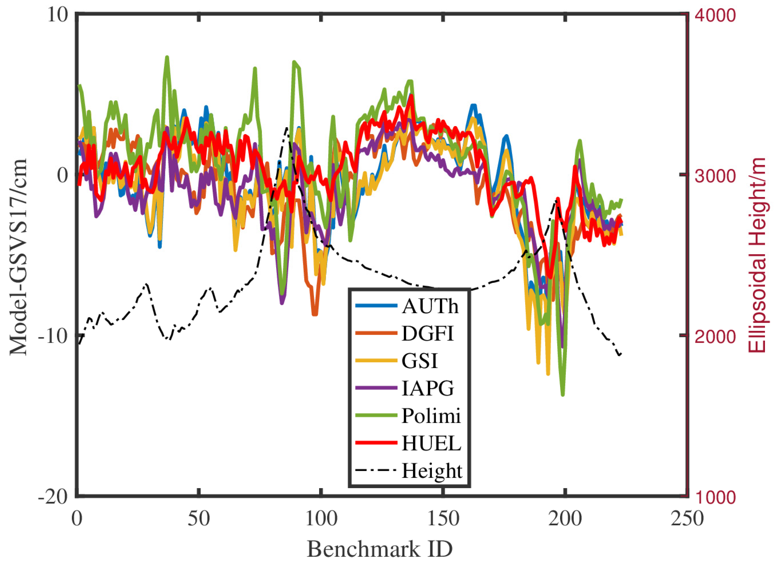
(3) Compared with ColSRBF2019, ColUNBSH2019, ColRLSC2019, and ColWLSC2020 submitted to ISG by different institutions, the ColSRBF2023 model showed a reduction in the STD value of approximately 0.2–1.6 cm with respect to the GSVS17 data.
(4) Comparisons are also made with the mean geoid model of ISG. ColSRBF2023 for the whole target area delivers an STD value of 2.4 cm, which is also a small value for all participants. Moreover, there is favorable agreement between the STD value with respect to the area mean solutions and the STD with respect to the GSVS17 GPS/leveling data, which shows the reliability of our geoid model ColSRBF2023 to a certain extent.
Overall, in this study, we aimed to enhance the quality of the geoid model in Colorado using band-limited SRBFs. To achieve this, the investigation and determination of the optimal expansion degrees for both terrestrial and airborne gravity data were conducted. The optimal geoid model was obtained when the maximum expansion degrees for terrestrial and airborne gravity data were determined to be 5200 and 1840, respectively, while the minimum expansion degrees for both data types were set to 720. The study demonstrated the significance of accurately determining the spectral information of gravity data, particularly in rugged areas. In future studies, we plan to perform further analyses of the remaining error sources in the determination of geoid models based on band-limited SRBFs, including the effect of the cutoff degree of the GGM, topographic reductions, and different approaches to handling airborne data, thereby furthering our contribution to the 1 cm geoid experiment of Colorado.


