Article

Background Reconstruction via 3D-Transformer Network for Hyperspectral Anomaly Detection

1
Key Laboratory for Information Science of Electromagnetic Waves (MoE), Fudan University, Shanghai 200437, China
2
Image and Intelligence Laboratory, School of Information Science and Technology, Fudan University, Shanghai 200437, China
*
Author to whom correspondence should be addressed.
Remote Sens. 2023, 15(18), 4592; https://doi.org/10.3390/rs15184592
Submission received: 16 August 2023 / Revised: 11 September 2023 / Accepted: 15 September 2023 / Published: 18 September 2023

Abstract

:
Recently, autoencoder (AE)-based anomaly detection approaches for hyperspectral images (HSIs) have been extensively proposed; however, the reconstruction accuracy is susceptible to the anomalies and noises. Moreover, these AE-based anomaly detectors simply compress each pixel into a hidden-layer with a lower dimension and then reconstruct it, which does not consider the spatial properties among pixels. To solve the above issues, this paper proposes a background reconstruction framework via a 3D-transformer (3DTR) network for anomaly detection in HSIs. The experimental results on both synthetic and real hyperspectral datasets demonstrate that the proposed 3DTR network is able to effectively detect most of the anomalies by comprehensively considering the spatial correlations among pixels and the spectral similarity among spectral bands of HSIs. In addition, the proposed method exhibits fewer false alarms than both traditional and state-of-the-art (including model-based and AE-based) anomaly detectors owing to the adopted pre-detection procedure and the proposed novel patch-generation method in this paper. Moreover, two ablation experiments adequately verified the effectiveness of each component in the proposed method.

1. Introduction

Hyperspectral images (HSIs) are collected by sensors on airborne or space platforms that combine imaging and spectroscopy techniques, and can be regarded as 3D data cubes. Apart from 2D spatial information, each pixel of an HSI with hundreds of bands can be regarded as a spectral vector [1,2]. Moreover, when disregarding subtle spectral variability, each material has a corresponding spectral curve, which gives HSIs a unique advantage in practical applications such as classification [3,4], unmixing [5], target detection [6,7] and denoising [8,9].
It is worth noting that HSIs are only a mixture of several endmembers due to the limitation of the category numbers of materials in real reality [10]. Therefore, the spectral curves of pixels, especially spatially adjacent pixels, are similar. In other words, there are spectral similarities among pixels from the spatial dimension [11]. For the sake of simplicity, the “spatial similarity” is utilized to represent this spectral similarity among pixels on the spatial dimension. In addition, the hundreds of single-band images are highly similar intuitively, namely, there is a global spatial similarity from the spectral dimension. Likewise, the “spectral similarity” is utilized to represent this global spatial similarity among bands on the spectral dimension.
According to whether the prior spectral information of a target is known, hyperspectral target detection can be divided into supervised and unsupervised types. Unsupervised target detection is also known as anomaly detection, which detects uncommon objects with significant different spectra from the background. Considering the difficulty of obtaining the specific spectral curves of a target, anomaly detection should be more consistent when used in practical applications, such as environmental supervision [12], mineral exploration [13,14], search and rescue [15,16], and military reconnaissance [17,18].
Various hyperspectral anomaly detection methods have been proposed in recent decades. Among these, the most typical method for anomaly detection is the Reed–Xiaoli (RX) detector [19], which detects anomalies by computing the Mahalanobis distance between the mean of the background and the tested pixel under the assumption that the background obeys a multivariate Gaussian distribution. However, this assumption is difficult to satisfy in real HSIs, which results in unsatisfactory detection results. To avoid making assumptions about the distribution of the background, the collaborative-representation-based detector (CRD) [20] considers that the anomalies cannot be represented by their spatial neighbors inside the man-set outer window, whereas the background pixels can. Unfortunately, there is no general rule for choosing the proper dual-window size for HSIs, which limits the accuracy of this detector in real applications. Moreover, the anomalous level for each pixel is computed separately in RX-based detectors and CRD; thus, the global statistic properties of the entire HSIs are ignored.
Recently, robust principal component analysis (RPCA) [21] were utilized to handle hyperspectral anomaly detection with low-rank background and sparsity of anomalies [22]. Later, low-rank representation (LRR) [23] was used to impose low-rank regularization on an abundance matrix correlated with a background dictionary; the inherent subspace structures of complex HSIs were then recovered. Considering that each pixel of an HSI can be represented by only a few dictionary atoms, low-rank and sparse representation (LRASR) [24] incorporated the l 1 -norm on each column of the abundance matrix based on LRR. In addition, the graph and total variation (TV)-regularized LRR (GTVLRR) [25] incorporated graph and TV regularizations to characterize the spatial properties of the background; thus, a relatively good decomposition result was obtained. An anomaly detector with a local spatial constraint and total variation (LSCTV) [26] was used to make the pixels’ abundances of background close in each superpixel. However, the complex distribution of the actual background in real HSIs is difficult to describe with a simple specific model; thus, the accuracies of the above model-based anomaly detectors are limited.
Compared with the above model-based detectors that seek to describe the background and anomalies with specific models in detail, most of the neural network (NN)-based anomaly detectors simply reconstruct the background by only considering the spatial sparsity of anomalies. Owing to its excellent accuracy in the extraction of principal components, the autoencoder (AE) [27] was introduced to solve hyperspectral anomaly detection. An AE-based hyperspectral anomaly detector called HADGAN [28] introduced the generative adversarial network [29] to enhance the constraints on reconstruction errors to obtain better reconstruction accuracy of the background. In addition, a robust graph AE (RGAE) [30] added the graph regularization on a hidden layer of each superpixel to consider the correlation among pixels. However, the above AE-based detectors have a common drawback in that the accuracy of the background reconstruction is susceptible to the anomalies. In terms of this issue, SSLGAN [31] alleviated the contamination of anomalies on the training procedure through the use of coarse screening. For the same purpose, GAED [32] generated a guided image to suppress the participation of anomalies. Unfortunately, the spatial properties between pixels are absent in most of the AE-based anomaly detectors, which is vital for reconstructing an accurate background.
In a word, the following problems with the aforementioned hyperspectral anomaly detectors need to be solved: (1) traditional specific model-based algorithms show instability across various datasets; (2) most of the NN-based detectors do not take spatial properties into account and easily suffer from the contamination of anomalies as well as noise; and (3) Both the spectral similarity of HSIs and the spectral dimension have been shown to improve the accuracies of hyperspectral anomaly detectors due to the global spatial similarity among hundreds of single-band images; however, these are not considered in all NN-based detectors.
To solve the abovementioned problems, this paper proposes a background reconstruction framework via a 3D-transformer network for anomaly detection in HSIs. Compared with AE-based algorithms that reconstruct each individual background pixel by compressing it into a hidden layer, the proposed network utilizes the transformer (TR) [33] module to handle the background pixel reconstruction with other pixels to effectively characterize the spatial correlations among pixels. Considering that hundreds of single-band images show high spectral similarity, a spectral TR network is presented to excavate this unique high-dimensional information of HSIs. By using this 3DTR network, which is combined with a traditional spatial TR and the proposed spectral TR in series, the background component of HSIs can be reconstructed effectively. Further, to reconstruct the background more precisely, the pre-detection of anomalies is executed by a simple but efficient anomaly detector so that the training procedure can be less contaminated by the pre-removed potential anomalies. To improve the reconstruction accuracy in each patch, a novel patch-generation method is proposed, in which a patch is generated by picking out the most similar pixels around the center pixel within a relatively wide range. Unlike traditional patch-generation methods [34,35,36] that include all the pixels around the center pixel within a pre-set single window, the proposed patch-generation method can alleviate the contamination of weakly relevant and irrelevant pixels during the reconstruction procedure of each patch. After a sufficient training procedure by the proposed 3DTR network, an accurate detection result can be obtained by means of the reconstruction errors of the whole HSIs.
It is worth noting that the strategy of using spatial TR and spectral TR has been utilized in change detection (SSTTR) [37]. However, the purpose of the two TRs used in SSTTR is to only extract the features; the results of the change detection procedure are obtained by comparing the extracted features of two HSIs. The strategy is thus different to the strategy proposed in this paper, which is to reconstruct a precise background using 3DTR. Moreover, SSTTR adds linear projections in front of two TR, which subjectively changes the dimensions of the input. As a result, the two TRs in SSTTR do not actually characterize the correlations among pixels and the correlations among bands, and the action mechanism is completely different to that of the 3DTR proposed in this paper. In addition, TR is has been utilized in hyperspectral anomaly detection (S2DWMT) [38]. However, S2DWMT only extracts features from a spatial perspective, whereas the 3DTR proposed in this paper extracts features from both spatial and spectral perspectives.
The main contributions of the proposed method can be summarized as follows:
(1)
A 3DTR network is proposed for hyperspectral anomaly detection that aims to reconstruct the background precisely by reflecting the multi-dimensional similarity in HSIs. Specifically, the TR module is utilized to handle the similarity among pixels, which is beneficial for the reconstruction of background compared to AE-based anomaly detectors that handle each pixel separately. Moreover, by fully considering the high spectral resolution of HSIs and the high spectral similarity among single-band images, a novel spectral TR network is proposed to reconstruct each band by other bands. To our knowledge, this is the first time that spectral similarity has been characterized among hundreds of single-band images by a TR module for hyperspectral anomaly detection;
(2)
In view of the potential contamination of anomalies in the reconstruction results of the background, a pre-detection procedure for anomalies is executed so that the potential anomalies can be removed in the training process of the 3DTR. Existing patch-generating methods simply set a single window around the tested pixel and regard all pixels in this window as a patch, which may include a number of irrelevant pixels and affect the precision of the background reconstruction. To solve this problem, a novel patch-generation method is proposed to select the most similar pixels around the center pixel in each patch, so that contamination from weakly relevant and irrelevant pixels in the background reconstruction are significantly reduced.
The remainder is arranged as follows. Section 2 briefly describes the related works. The proposed method is presented in detail in Section 3. In Section 4, the experimental results of the two synthetic datasets and six real datasets are shown and analyzed. Finally, the conclusions are drawn in Section 5.

2. Related Works

It is well known that TR [33] is used to handle the sequence-to-sequence translation problems in natural language processing (NLP). Recently, TR has been widely used in various vision tasks, in which the pixels or patches of images are processed into sequences as the input of TR. The unique long-range self-attention mechanism of TR excavates the interrelations among these sequences, allowing each sequence to capture the global information. Therefore, the TR module is actually a similarity-based reconstruction network, which produces better results in vision tasks such as human pose estimation [39], segmentation [40,41], target detection [42,43] and image classification [44,45].
A traditional TR module is composed of a layer normalization (LN), a multi-head self-attention (MSA), and a multiple layer perception (MLP), as shown in Figure 1a. Particularly, the MSA module shown in Figure 1b is stacked by several self-attention (SA) blocks (heads) shown in Figure 1c, which play a crucial role in excavating the interrelations among sequences. Specifically, a head can be carried out according to the following steps:
Step 1: 
the input x i R L × 1 , i = 1 , , N is an arbitrary sequence with L elements, which is processed from a pixel or a patch of the tested image. To avoid the shortcoming where the position information is missed by the self-attention mechanism, an artificial or random position code is added to the original input: x i = x i + p i R L × 1 , i = 1 , , N .
Step 2: 
each input is multiplied by three pre-set transformation matrices W q R M × L , W k R M × L , and W v R M × L , respectively. Three corresponding vectors are obtained, i.e., query q i R M × 1 , key k i R M × 1 , and value v i R M × 1 .
Step 3: 
the attention score s i , j is calculated between the input x i and other arbitrary input x j by the above transformed vectors, i.e., s i , j = q i T · k j / L .
Step 4: 
The softmax activation layer is operated on the attention score s i R N × 1 .
Step 5: 
the attention output is computed z i = j s i , j v j R M × 1 .
To summarize, the output of a head for x i can be integrated into the following formulation:
z i h = SA q i , k i , v i = softmax q i k i T L v i R M × 1
where h = 1 , , H denotes the h-th head in the MSA module, so that different positions can be focused on, and the accuracy of self-attention is enhanced. Then, the stacked output of the MSA module for x i can be transformed by W R L × H M as follows:
z i = W z i 1 ; ; z i M R L × 1 .

3. Proposed Method

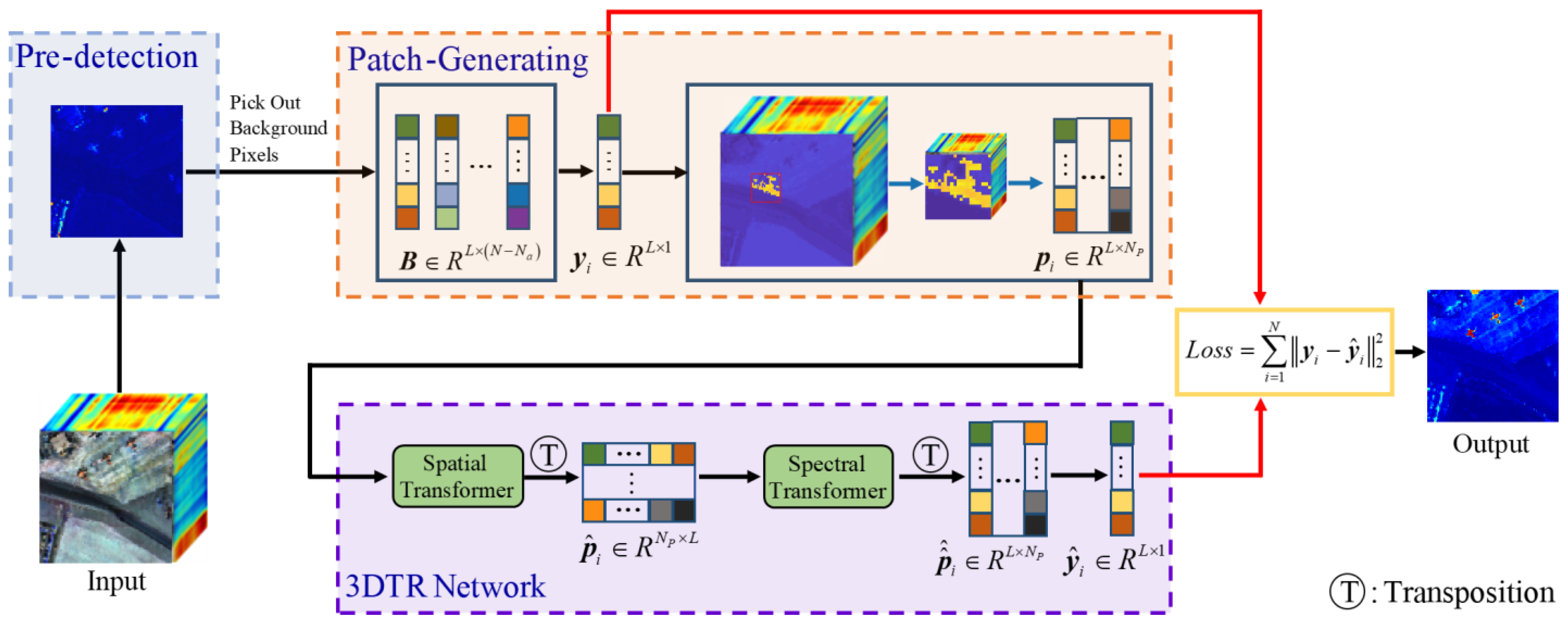
This paper proposes a novel hyperspectral anomaly detector, which is based on the fact that the anomalies have several obvious characteristics: a small quantity, sparse distribution, and spectral difference with their neighbors. In other words, a background can be well characterized by the proposed 3DTR network, and then the pixels with relatively large reconstruction errors can be regarded as anomalies. Specifically, the proposed method is composed of four major procedures: a search of the representative background pixels by a coarse anomaly detector; the construction of patches by the proposed patch-generating method; training of the proposed 3DTR network using only the searched background; and testing of the original HSIs by the trained 3DTR network. The overall schematic of the proposed method is illustrated in Figure 2.

3.1. 3DTR Network for Anomaly Detection

Let D = d 1 , d 2 , , d N R L × N denote the 2D hyperspectral data matrix with N pixels and L spectral bands, which is also regarded as the testing dataset. Then, D is severed by a coarse anomaly detector to A = a 1 , a 2 , , a N a R L × N a a n d B = b 1 , b 2 , , b N N a R L × N N a , which denote the potential anomalies and the representative background, respectively. Each pixel of the training dataset B generates an independent patch as the input of the proposed 3DTR network. The specific processes of the coarse anomaly detector and the proposed patch-generating method will be introduced in the following subsections.
As mentioned previously, pixels, especially spatially adjacent pixels, in the HSIs are spatially similar because of the limit in the category number of materials in reality. In other words, each background pixel can be represented by its relevant neighbors. Therefore, the TR module can be utilized to reconstruct each pixel with other similar pixels due to its unique long-range self-attention mechanism, which suppresses the heterogeneous noise and spectral variation.
It is regrettable that all the above examples for vision tasks extract pixels or patches of a tested image as the inputs of the TR module, and therefore only consider the spatial interrelations. However, the spectral similarity among spectral bands in HSIs is more conspicuous, and each single-band image can apparently be represented by other single-band images. Therefore, to enable the TR module to more deeply excavate information about the HSIs, and make the process more suitable for real applications of HSIs, it was proposed that the spectral TR module would first reconstruct each single-band image using other single-band images, which fully exploit the spectral interrelations of HSIs.
Without a loss of generality, let us take y i as an example to demonstrate the following processes of the 3DTR network, which could be an arbitrary pixel in training dataset B or testing dataset D.
Step 1: 
By considering that the neighboring region of y i is more important in the reconstruction process compared to the whole HSIs, this paper uses a patch rather than the whole HSI to generate the reconstructed pixel y ^ i . Moreover, to avoid contamination by uncorrelated pixels, the proposed patch-generating method generates a one-to-one corresponding patch p i R L × N P by selecting N P highly correlated pixels around y i , in which y i comes first in p i .
Step 2: 
Input p i to the h 1 -head TR module, in which each pixel of p i is considered as an input sequence. By considering the interrelations among pixels, the patch p ^ i R L × N P is reconstructed by this spatial TR module.
Step 3: 
To characterize the spectral similarity among spectral bands of HSIs, the transposed patch p ^ i T R N P × L is fed into the h 2 -head TR module, in which each band of p ^ i is considered as an input sequence. By considering the interrelations among spectral bands, the transposed patch p ^ ^ i T R N P × L is reconstructed by this spectral TR module.
Step 4: 
Then, the first column of the reconstructed patch p ^ ^ i R L × N P is the reconstructed pixel y ^ i .
The specific network configurations are listed in Table 1. After repeating the above steps on all pixels and their corresponding patches of training dataset B, the loss function can be formulated as:
L o s s = i = 1 N y i y ^ i 2 2 = i = 1 N y i 3 DTR y i 2 2 .
Finally, the HSI D ^ is reconstructed by the trained 3DTR network. It is worth pointing out that the proposed 3DTR network only learned the characteristics of background owing to the removal of potential anomalies in the pre-detection process. In other words, the background can be well reconstructed by the trained 3DTR network, whereas the anomalies cannot. Thus, the anomalous value of an arbitrary pixel y i can be computed by the reconstruction error as:
y i 2 2 = y i y ^ i 2 2 = l = 1 L y i l y ^ i l 2 .

3.2. Removing Potential Anomalies

To avoid contamination by anomalies in the training procedure, and provide rough labels for inputs in the meantime, a simple and efficient anomaly detector is adopted to handle the coarse pre-detection on the original HSIs, in which the first N a pixels are marked as potential anomalies. Therefore, by the means of the coarse pre-detection, the potential anomalies are preliminarily dislodged, and a relatively purified background dataset, namely, the training dataset B, can be constructed. In addition, due to the limitations of the pre-detection performance, some of the background pixels are also inevitably removed by setting a relatively loose threshold. Owing to the similar features between the removed background pixels and the reserved pixels, the well-trained network is able to reconstruct the removed background pixels by learning the similar features of other reserved background pixels. Therefore, the small amount of background pixels removed in the pre-detection process do not affect the detection performance, which is further demonstrated in the experiments of generalization evaluation.
According to the physical definition of anomalies that the proportion of anomalies is usually quite low in HSIs, the anomalies can be dislodged by setting a relatively relaxed threshold. Specifically, the N a is set to 300 in all the following experiments, which is much greater than the quantity of anomalies in practical HSIs. Therefore, the requirement for accuracy in the pre-detection process is relatively low; any efficient anomaly detector can be utilized for the pre-detection process described in this paper.

3.3. Patch-Generating

The long-range self-attention mechanism of TR module can consider the pairwise interrelations of all inputs but feeding tens of thousands of pixels of HSIs into the TR module at the same time is extremely time-consuming. Therefore, this paper proposed to generate a patch around the tested pixel and use the pixels in this patch as the inputs of the TR module.
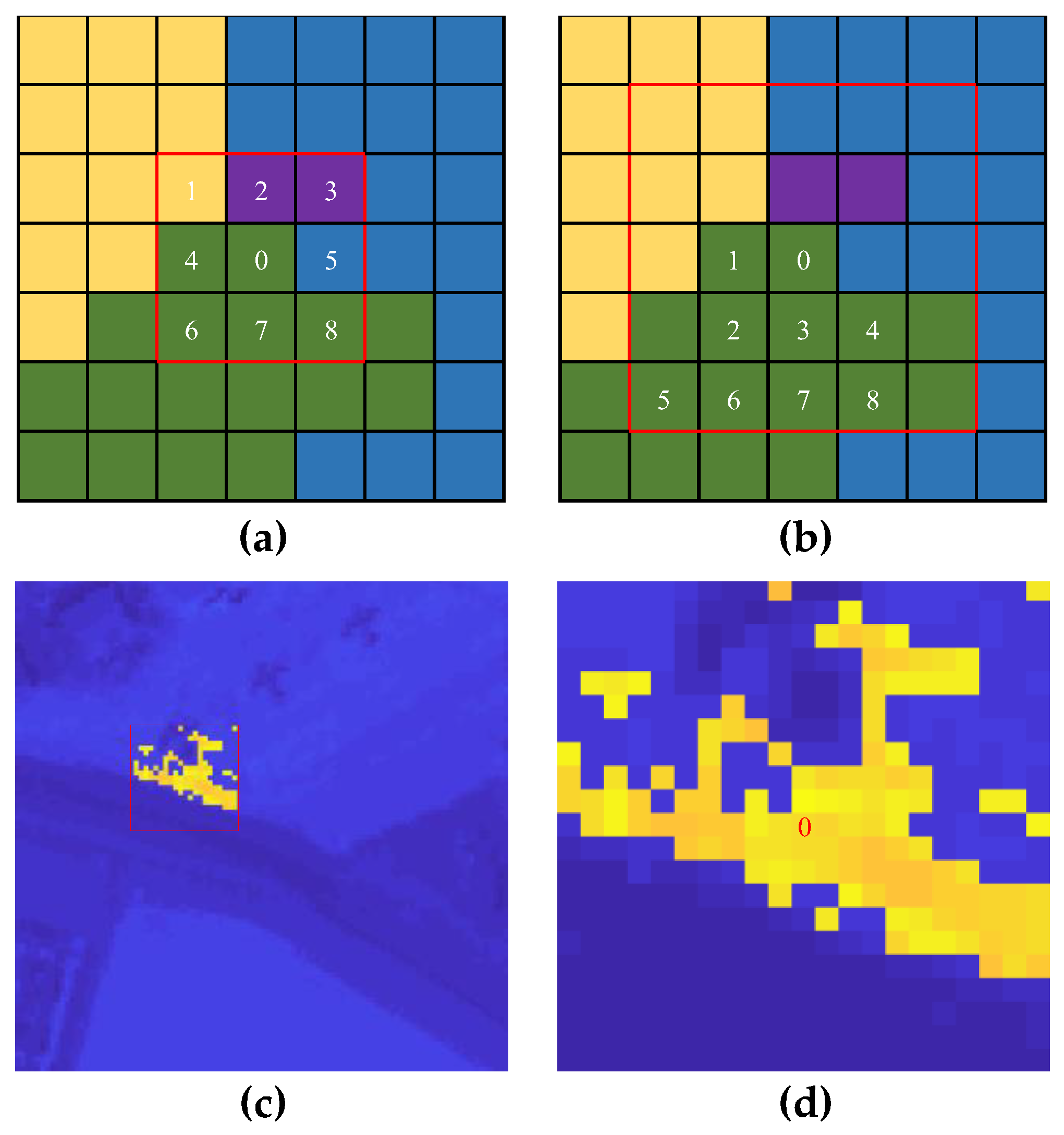
Let the sketch map with 7 × 7 -pixels denote the trimmed hyperspectral imagery shown in Figure 3, in which green, yellow and blue denote three categories of background and the purple denotes the anomalies. It is regrettable that most of the existing patch-generating methods just simply set a single window around the tested pixel (0-th green pixel) and regard all pixels in this window as a patch, as shown in Figure 3a. As previously mentioned, the TR module actually realizes the similarity-based reconstruction of pixels in the HSIs, and thus this simple patch-generating method introduces a number of irrelevant pixels into this well-shaped patch, and then influences the reconstruction results of the center pixel. As shown in Figure 3a, two irrelevant background pixels (1-th yellow pixel and 5-th blue pixel), and even some anomalies (2-th and 3-th purple pixels), are included in the single window.
To avoid the influence of irrelevant pixels and anomalies in the reconstruction procedure, a patch-generating method is proposed to coordinate the similarity-based reconstruction mechanism of the TR module. As shown in Figure 3b, a relatively large window is set around the tested pixel to impose restrictions on the spatial positions of other pixels participating in the reconstruction process. Then, using N P , which is set to 100 (only 9 pixels in Figure 3a,b for facilitating visual understanding), high-similarity pixels around the tested pixels are selected to compose the indeterminately shaped patch. In other words, only pixels with small spatial and spectral distances from the tested pixel can be selected to participate in the reconstruction process of the tested pixel to realize a better reconstruction result in the TR module. A real example is shown in Figure 3c,d, where a relatively large window is set around the center pixel and only similar pixels are selected to compose the patch, in which the irrelevant pixels of roads and the anomalous pixels of airplanes are all avoided.

4. Experimental Results and Analysis

In this section, two synthetic hyperspectral datasets with different abundances of anomalies are used to evaluate the detail processes and the performance of the proposed method comprehensively. Then, six varied real datasets are utilized to validate the effectiveness of the proposed method in practical applications.
In the following experiments, the three-dimensional receiver operating characteristic (3D ROC) curve [46], the abridged two-dimensional receiver operating characteristic (2D ROC) curves, and the area under the ROC curve (AUC) are adopted to intuitively evaluate the detection accuracies of the proposed method and other competitors of anomaly detection. Specifically, the 3D ROC curve is plotted by three metrics: threshold τ, false alarm rate P F , and detection rate P D . These can be used to draw 2D ROCs to each other and compute the corresponding AUC values, which are AU C D , F , AU C F , τ and AU C D , τ , respectively. Furthermore, five additional AUC values, denoted as AU C BS , AU C TD , AU C SNPR , AU C TD - BS and AU C OD , are calculated by the abovementioned three AUC values as follows:
AU C BS   = AU C D , F AU C F , τ AU C TD = AU C D , F + AU C D , τ AU C SNPR = AU C D , τ AU C F , τ AU C TD - BS = AU C D , τ AU C F , τ AU C OD = AU C D , F + AU C D , τ AU C F , τ
where AU C D , F , AU C TD - BS and AU C OD are adopted to evaluate the overall performances of anomaly detectors. AU C F , τ , AU C BS and AU C SNPR are adopted to evaluate the background suppressibility of detectors. AU C D , τ and AU C TD are adopted to evaluate the anomaly detectability of detectors. The smaller the AU C F , τ , the better the detector; other AUCs do the opposite.
All the experiments are executed by MATLAB R2018b and Pycharm 2021.3.2 on a personal computer with an Intel Core i9-11900K CPU at 3.5 GHz and 32 GB RAM.

4.1. Synthetic Data Experiments

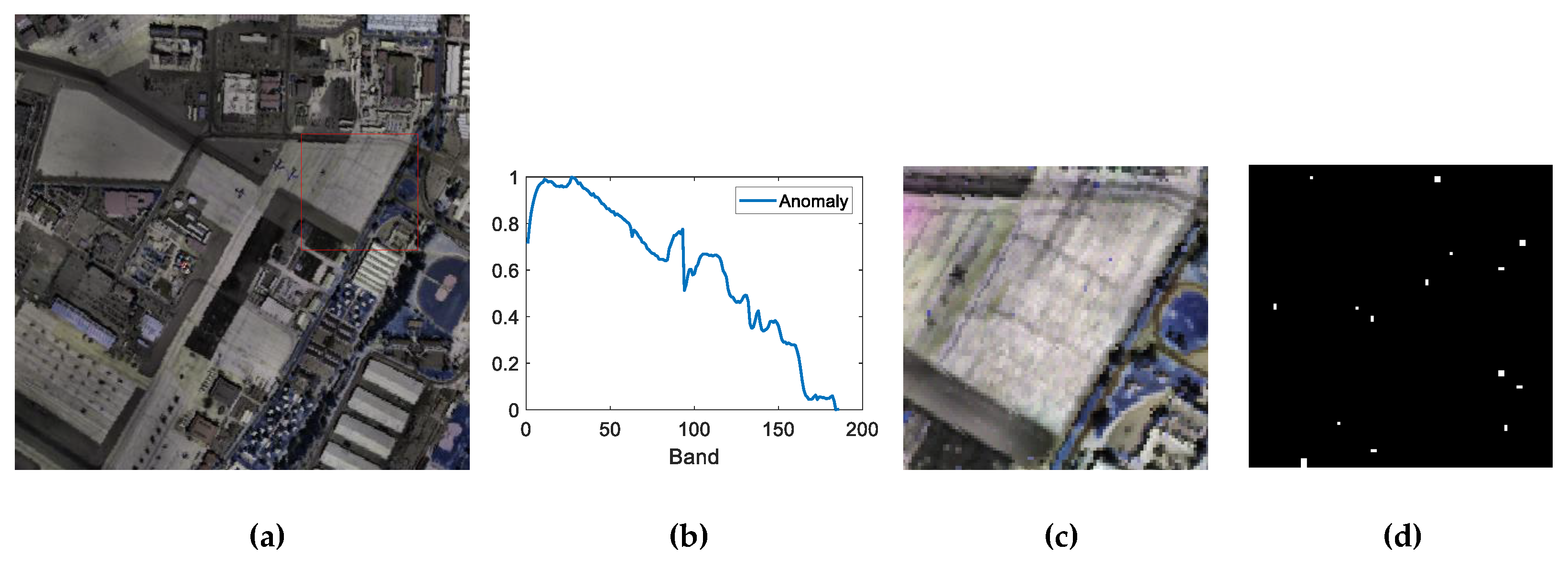
The two synthetic datasets used in this paper are generated based on real hyperspectral imagery collected from San Diego airport by the Airborne Visible/Infrared Imaging Spectrometer (AVIRIS). The incipient dataset contains 224 spectral bands but only 186 of them were retained in the following experiments after eliminating the low signal-to-noise-ratio (SNR) and water vapor absorption bands (i.e., 1–6, 33–35, 94–97, 107–113, 153–166, and 221–224). As is shown in Figure 4a, the original whole image has a size of 400 × 400 and a subimage with a size of 100 × 100 (in the red square) is trimmed to generate the synthetic datasets. The anomaly pixel with a spectral signature t is selected from an airplane in the pristine whole image, which is plotted in Figure 4b. Here, the synthetic anomaly pixel z is produced by proportionally embedding the selected anomaly spectra t into a random background spectra b on the basis of the linear mixing model, according to the target implantation method [47]:
z = f t + 1 f b
where f is the embedding proportion. Four anomaly blocks with different sizes of 1 × 1 , 2 × 1 , 1 × 2 and 2 × 2 are generated for each level of f . In addition, to accord with the real distributions of anomalies in HSIs, the positions of these generated anomaly blocks are entirely random.
Here, two synthetic datasets with different abundances are generated. Specifically, f belongs to 0.2 , 0.4 , 0.6 , 0.8 in the first synthetic dataset, and the pseudocolor image and the corresponding ground-truth map of the first synthetic dataset are displayed in Figure 4c,d, respectively. In the following experiments on the first synthetic dataset, several traditional and state-of-the-art (including model-based and AE-based) competitors are imported to reflect the detection superiority of the proposed method, and robustness to different levels of noise is demonstrated. Next, the multiple choices of the structure of the 3DTR network and the parameter settings of the pre-detection and patch-generating methods are compared and analyzed. Then, the generalization ability of the 3DTR network is evaluated. Moreover, to verify the detection accuracy of the proposed method in the case of weak signals, a second synthetic dataset with relatively low anomalous abundances ( f = 0.05 , 0.1 , 0.2 , 0.4 ) is generated to conduct the experiment assessing the method’s robustness to noise.
It is worth noting that the generated synthetic datasets are challenging for hyperspectral anomaly detection in three aspects: (1) the sizes of the anomalous blocks are varied, and their spatial locations are completely random; (2) the false alarms may be serious due to the sparse backgrounds existing in the scene; and (3) the anomalous abundances f are relatively low, especially in the second synthetic dataset, which is difficult for most anomaly detectors.

4.1.1. Experiments on the First Synthetic Dataset

Comparison of Detection Performances: To reveal the detection performance of the proposed method, four model- based anomaly detectors (RX [19], CRD [20], GTVLRR [25] and LSCTV [26]), and three AE-based anomaly detectors (AE [27], RGAE [30] and GAED [32]) are imported. RX is the most common anomaly detector, and assumes that the background obeys a multivariate Gaussian distribution. However, CRD aims to emphasize collaborative representation in the local regions. GTVLRR incorporates the graph and TV regularizations to the LRR-based decomposition model. LSCTV also introduces TV regularization in each superpixel to make the background abundances close. RGAE and GAED incorporate the graph regularization and the guided map based on AE, respectively.
The dual window size and the parameter λ are set to 3 , 7 and 10 6 in CRD, respectively, after extensive searching. For GTVLRR, this paper sets the involved parameters as λ = 0.5 , β = 0.2 and γ = 0.05 , as recommended in [25]. Similarly, this paper sets λ = 10 3 , β = 5 × 10 3 , P = 20 and S = 15 for the LSCTV, as recommended in [26]. In addition, the codes of RGAE [30] and GAED [32] were obtained from the authors. All the following experiments are implemented using shared source codes without any alteration. As mentioned above, any simple and efficient hyperspectral anomaly detector can be chosen for the pre-detection method; here, RX is adopted for its simplicity and efficiency.
The anomaly detection maps and the eight AUC values of the proposed method and competitors for the first synthetic dataset are shown in Figure 5 and Table 2, respectively. It can be observed that RX, CRD, AE and RGAE are not able to detect all the anomalies; in other words, the weak anomalies are challenging for these detectors, which is also demonstrated by the low AU C D , τ and AU C TD values of these detectors. In addition, the detection maps of GTVLRR, LSCTV and RGAE contain a large number of false alarms, which corresponds to their high AU C F , τ values. Owing to the strong suppression of the background by the guided map (optimal in AU C F , τ , AU C BS and AU C SNPR ), a relatively good detection result with scarcely any false alarms is obtained by GAED; however, several weak anomalies are also suppressed simultaneously, which results in relatively low detection accuracy and the second lowest values in AU C D , τ and AU C TD . Correspondingly, the proposed method in this paper achieved improved detection results, the highest values in AU C D , τ and AU C TD , and the best overall performance in AU C D , F , AU C TD - BS and AU C OD .
The 3D ROC curves and three abridged 2D ROC curves of all detectors are plotted in Figure 6 to evaluate the anomaly detection accuracies quantitatively. For nearly all false alarms and τ, the detection rate of the proposed method is higher than that of all competitors in Figure 6b,c. Moreover, a 100 0 0 detection rate is achieved when the false alarm rate is very low in the proposed method. In addition, the eight AUC values listed in Table 2 demonstrate the best detection accuracy and the best overall performance of the proposed method, quantitatively.
The time consumption of all anomaly detectors for the first synthetic dataset are also listed in Table 2. Compared with the time-saving detectors (RX, CRD, AE and GAED), the GTVLRR, LSCTV and RGAE incorporate different spatial regularizations, and improve the estimation of background in multiple iterations, which result in an apparent increase in time costs in these three algorithms. Similarly, the proposed method trains the network by patches of pixels in several epochs, which is also time-consuming. In addition, the test time of the proposed method is within an acceptable range, which indicates its capacity in practical applications.
For considering the brevity of the charts in the following numerous experiments, only the RO C D , F and the corresponding AU C D , F , which represent the overall performance, are utilized to evaluate the detection accuracies of all anomaly detectors.
Robustness to Different Levels of Noise: To verify the stability of the proposed method, different levels of Gaussian noise (20, 25 and 30 dB, respectively) are utilized to corrupt the first synthetic dataset. Here, the SNR is defined as follows:
SNR = 10 log 10 E y T y E n T n
where E · represents the expectation of the contents, y and n denote the incipient pixel and the added noise, respectively. It can be observed from the ROC curves in Figure 7 that the proposed method is still superior to other anomaly competitors for almost all false alarms and various levels of noise. Moreover, 20 replicates were performed for each level of noise, and the mean value and the corresponding standard deviation (std) of AU C D , F values are listed in Table 3. It is obvious that the proposed method is more robust in the case of noise corruption compared with other anomaly detectors, owing to the full consideration of the similarity among pixels and the global spatial similarity among bands by the two TR modules.
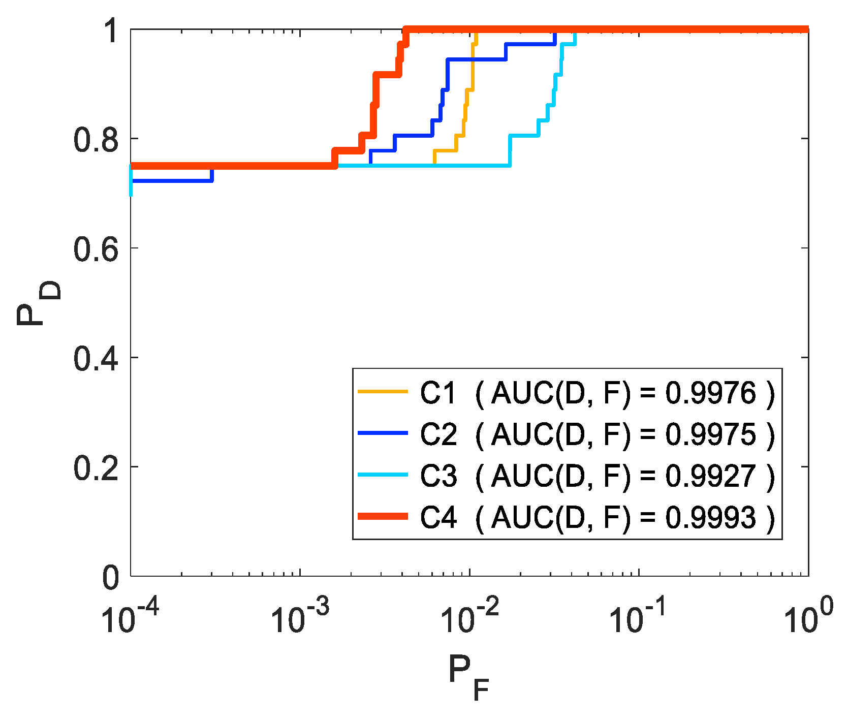
Ablation on Different Components: An ablation study is conducted to assess the contribution of each component in the proposed method. Specifically, four cases are listed in Table 4.
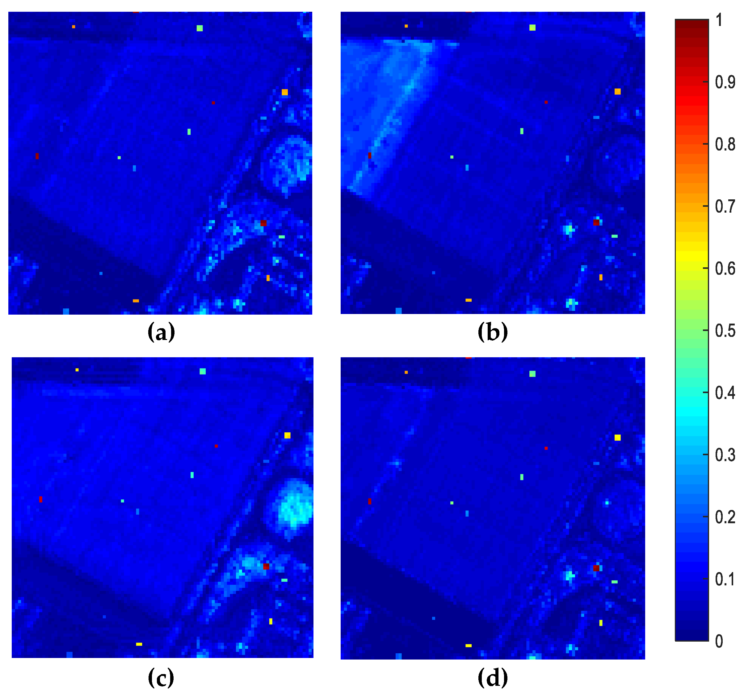
The anomaly detection maps, ROC curves and AU C D , F values are summarized in Figure 8 and Figure 9, respectively. As summarized in Figure 9, the AU C D , F values of C1 and C2 are relatively high, and in the meantime their anomaly detection maps show good anomaly detection accuracies using the single TR modules. However, the anomaly detection maps and ROC curves of C1 and C2 also indicate that there are quite a few false alarms in these two cases. To excavate the similarity of multiple dimensions in HSIs, C4 (the proposed method) connects two TR modules in series, which achieves an excellent anomaly detection accuracy and a relatively low number of false alarms. The ROC curve and AU C D , F value of C4 also demonstrate its superiority quantitatively. In addition, compared with the proposed patch-generating method in C4, C3 generates patches by setting single windows around pixels, resulting in false alarms due to the introduction of unrelated pixels.
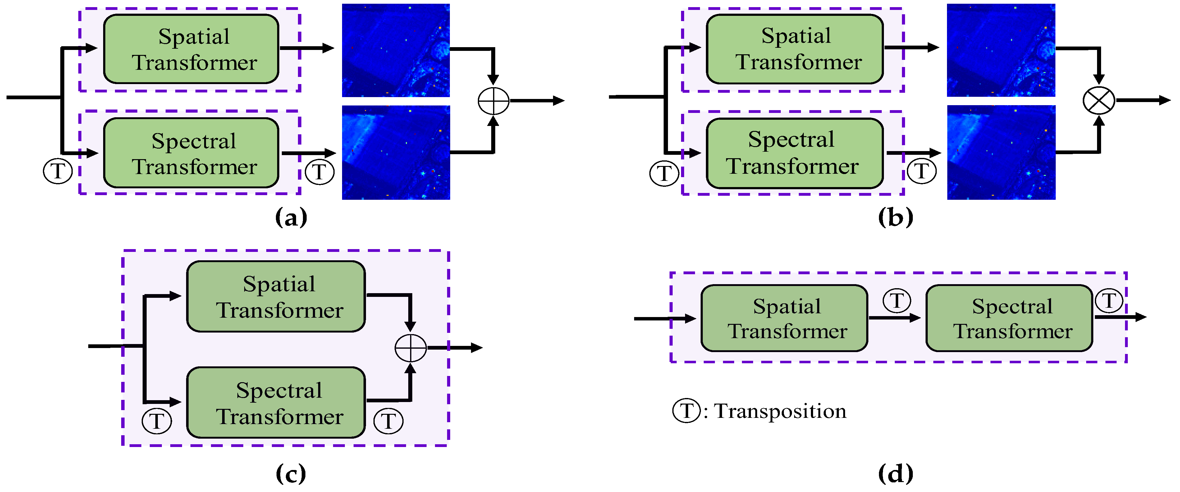
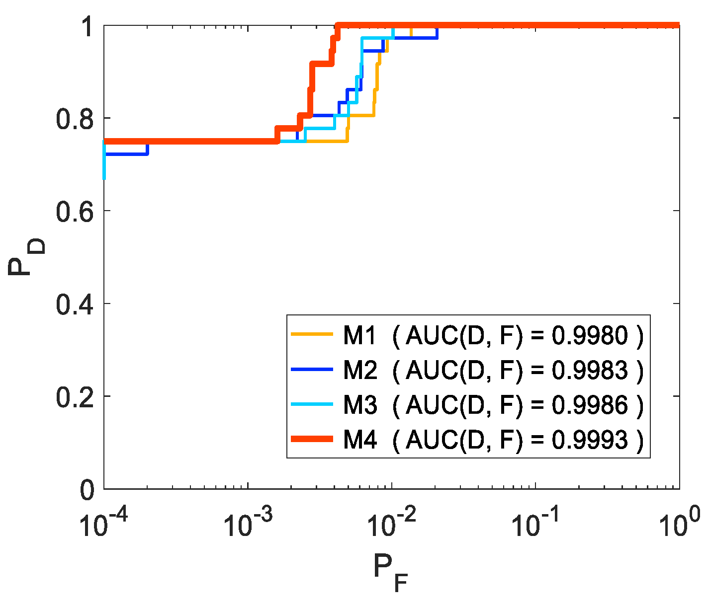
Ablation on Different Combination Modes: An ablation study is conducted to assess the accuracies of different combination modes of both TR modules. Analogously, four cases are listed in Table 4 under the premise of the proposed patch-generating method. In addition, the abbreviated flowcharts of four cases are shown in Figure 10, in which a purple dotted box denotes a standalone network.
Similarly, the anomaly detection maps, ROC curves and AU C D , F values are summarized in Figure 11 and Figure 12, respectively. To utilize the similarities of multiple dimensions in HSIs, M1 and M2 simply merge the detection results of spatial TR and spectral TR algebraically, without making a connection in the network structure, which does not fully integrate the advantages of two single TR modules, and the increases in the detection results of these two cases are limited. In addition, M3 realizes the connection of two TR modules in parallel anatomically; however, the mutual constraint between two TR modules in training process are relatively finite, which limit the detection accuracy of M3. Therefore, to reinforce the mutual constraint between two TR modules in network, this paper finally decides to connect two TR modules in series anatomically, namely, the proposed 3DTR network in this paper, and a superior anomaly detection result is obtained.
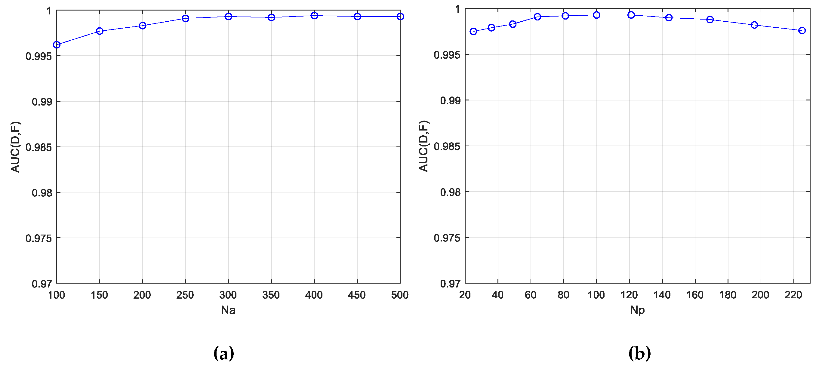
Parameter Setting:  N a is the parameter in pre-detection used to dislodge the potential anomalies prior to the training procedure. The value of N a ranges from 100 to 500, at intervals of 50, and the corresponding AU C D , F values are plotted in Figure 13a. In the case of small N a , the anomalies are not removed completely, and the reconstruction of the background is contaminated. Therefore, the detection accuracies are affected. On the other hand, because the number of anomalies is small and constant, the anomalies will not affect the background reconstruction when N a is relatively large. Thus, the AU C D , F value is almost a constant with the increase of N a . For the sake of simplicity, this paper fixes N a = 300 in the follow-up experiments.
Next, the influence of N P , namely the size of the patch, on the detection accuracies of the proposed method is analyzed. To match the size of the traditional square patch, the value of N P is set to the square of each value between 5 and 15, i.e., [25, 36, 49, 64, 81, 100, 121, 144, 169, 196 and 225], and the corresponding AU C D , F values are plotted in Figure 13b. The purpose of our patch is to provide similar pixels with which to reconstruct the center pixel. There are three cases to discuss: (1) when N P is too small, the number of similar pixels is insufficient to reconstruct the center pixel adequately; (2) when N P is too large, the irrelevant pixels and even anomalies may be included in the patch to affect the reconstruction of the center pixel; and (3) when N P is appropriate, AU C D , F values remains superior and stable over a relatively wide range. Therefore, this paper fixes N p = 100 in the follow-up experiments for the sake of simplicity.
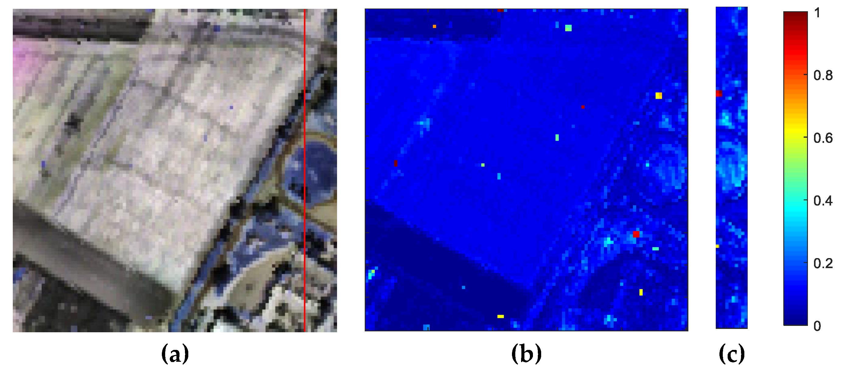
Generalization Evaluation: To comprehensively verify the generalization ability of the proposed 3DTR network, the first synthetic dataset is divided into a training set and validation set. Specifically, a subimage with a size of 100 × 90 to the left of the red line in Figure 14a (8875 pixels after removing potential anomalies) is regarded as the training set. Correspondingly, a subimage with a size of 100 × 10 to the right of the red line in Figure 14a (1000 pixels) is regarded as the validation set, and the original image is used as the testing set. It is worth noting that the proposed 3DTR network is trained only on the training set, and eventually tested on the validation set and the testing set.
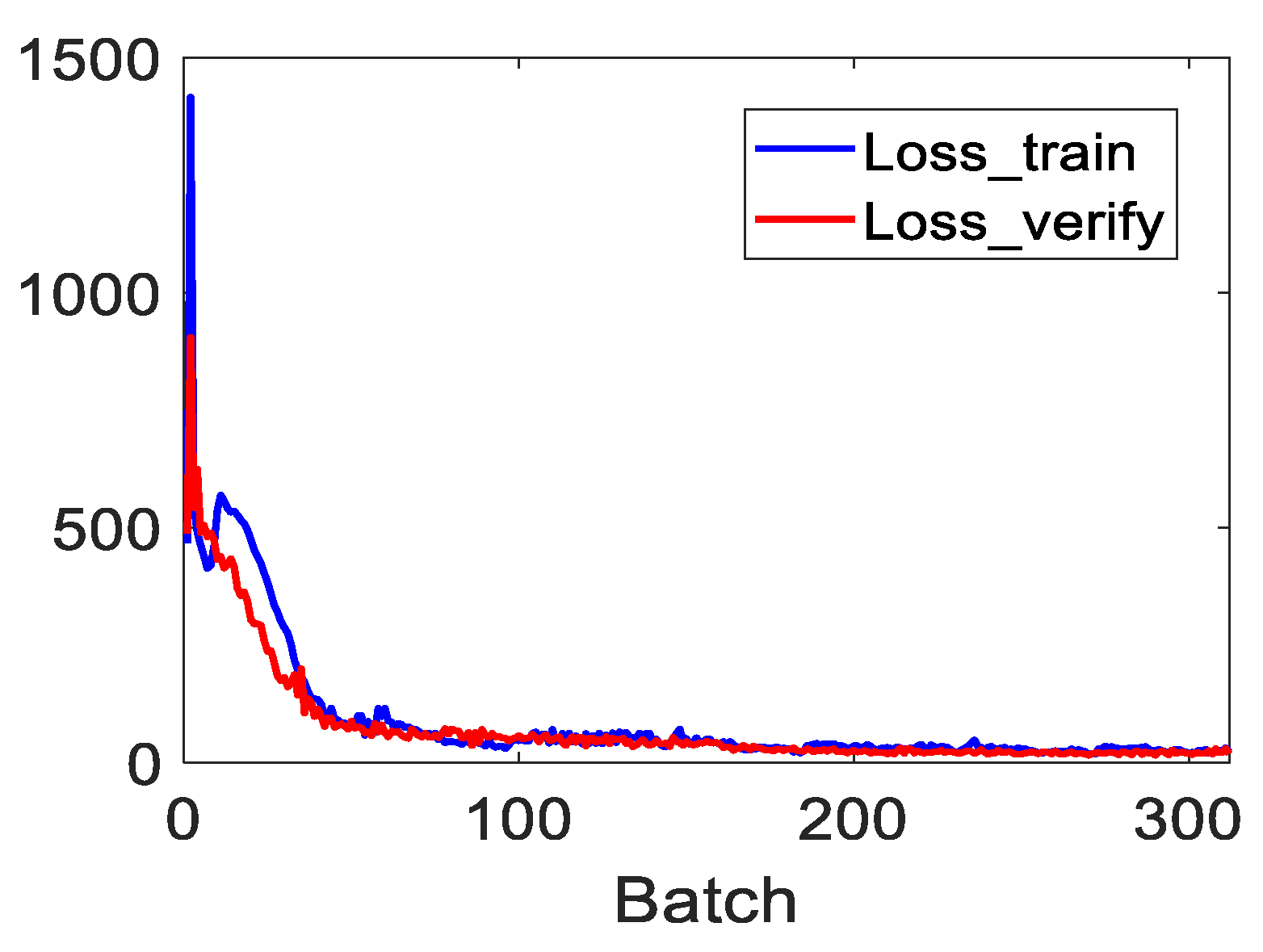
The loss curves of the network on the training set and validation set are shown in Figure 15, and it can be observed that the loss of the validation set decreases and stabilizes with the loss of the training set, which demonstrates the absence of the overfitting problem. Moreover, the detection maps of the partly trained 3DTR network on the validation set and the testing set are shown in Figure 14, and there is no obvious change when compared with the detection map of the fully trained 3DTR network in Figure 11d. In addition, the five anomalies in the validation set are detected faultlessly in Figure 14c, and the AU C D , F of the validation set is 1, which further verifies the generalization ability of the proposed 3DTR network.

4.1.2. Experiments on the Second Synthetic Dataset

Likewise, 20 replicates for each level of noise are performed in the case of weak signals. The ROC curves and AU C D , F values are summarized in Figure 16 and Table 5, respectively. Compared with the case of strong signals, the detection accuracies of all detectors show varying degrees of decline. Even so, Figure 16 and Table 5 confirm the proposed method’s robustness to noise in the case of weak signals and its ability to detect weak anomalies.

4.2. Real Data Experiments

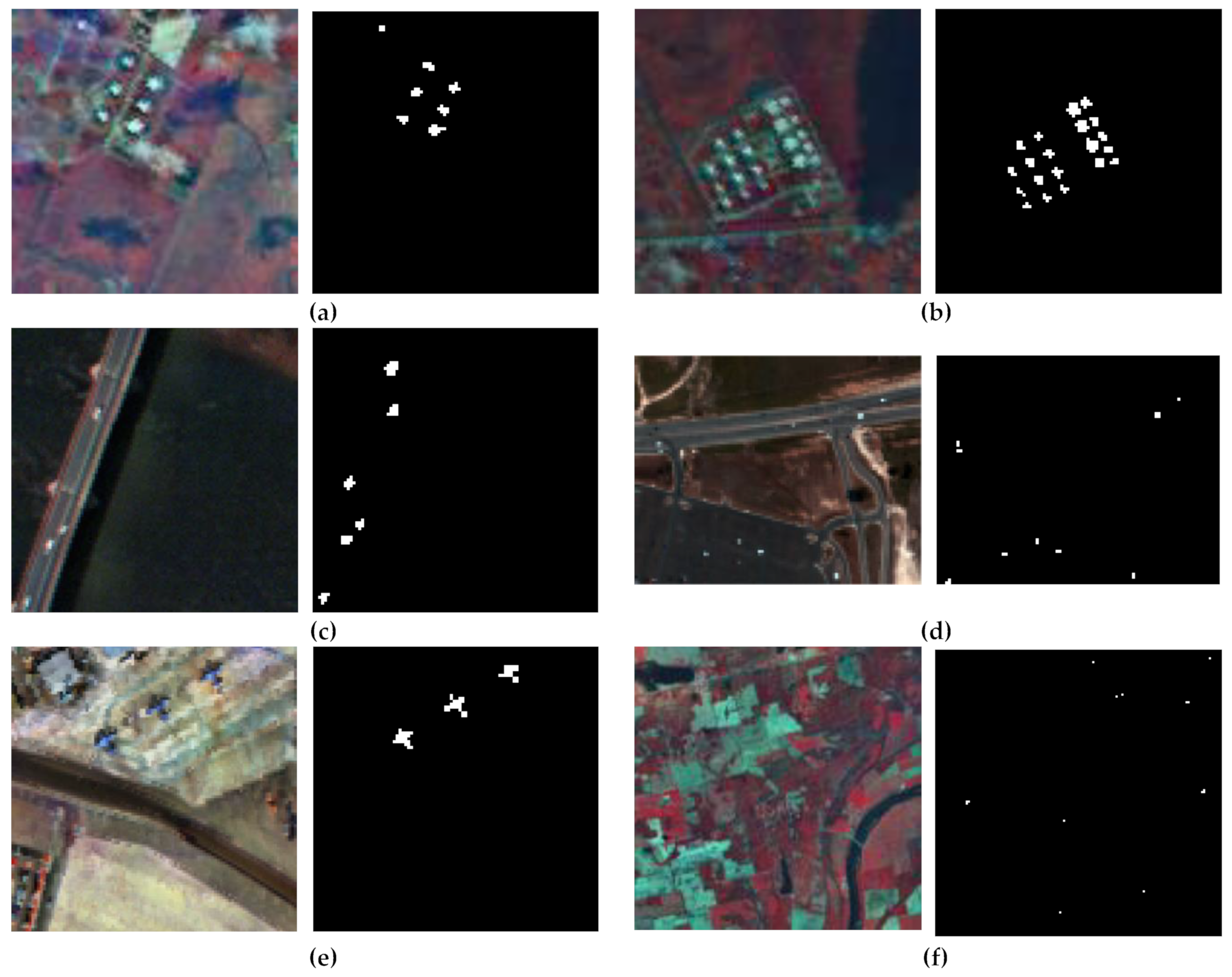
In this subsection, six widely used real hyperspectral datasets are applied to evaluate the detection accuracies of the proposed method and other competitors. The most important characteristics of the utilized six datasets are summarized in Table 6. And the pseudocolor images and their corresponding ground-truth maps of these six datasets are shown in Figure 17. It is worth noting that the window sizes of CRD for each dataset are also listed in Table 6, and that any other parameters of all detectors are set as described in the synthetic experiments.
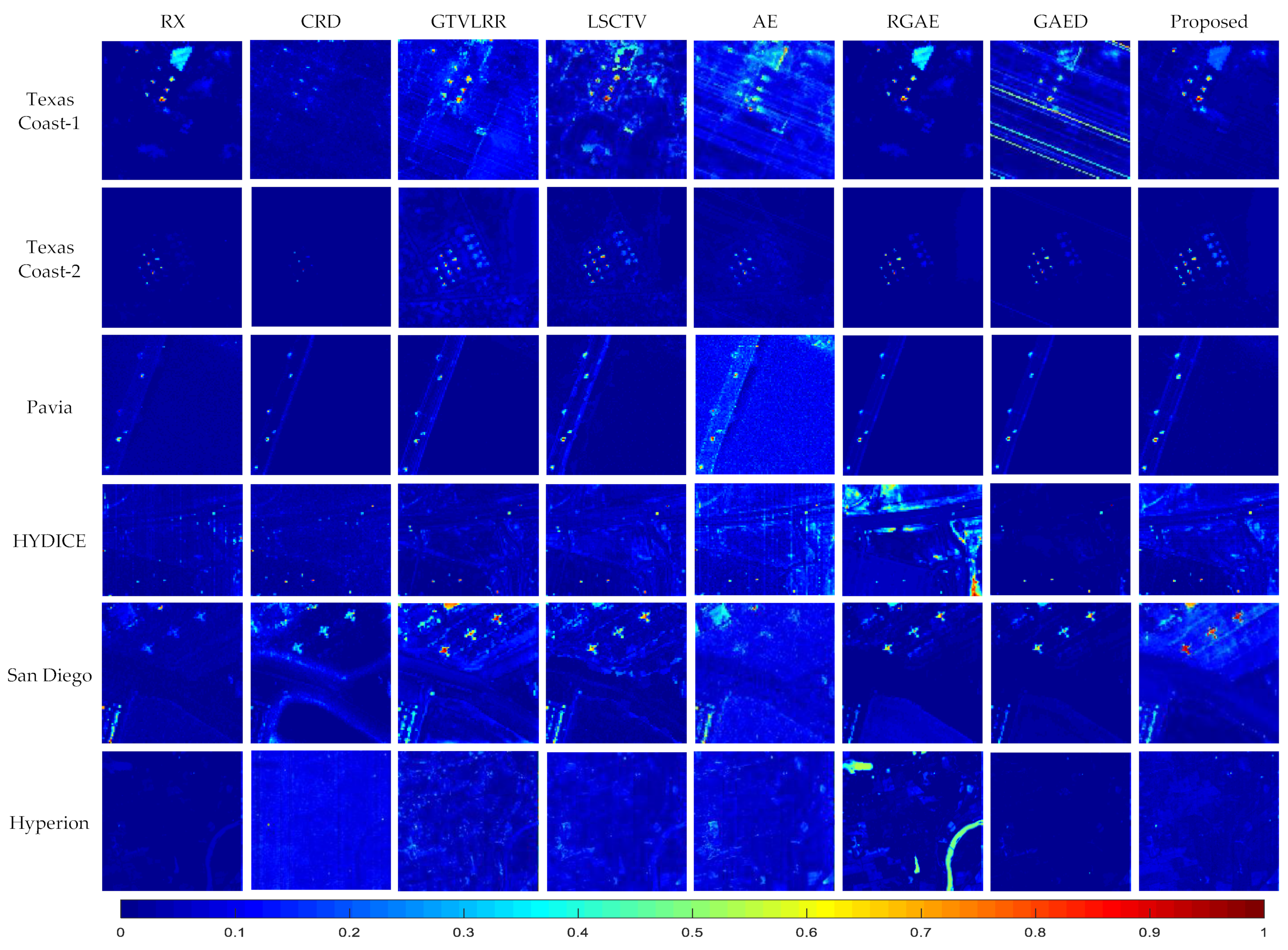
The detection results of all anomaly detectors on the six real datasets are displayed in Figure 18. Taking the first dataset (Texas Coast-1) as an example, the CRD and AE failed to detect all anomalies in the scene. Although RX, GTVLRR, LSCTV, RGAE and GAED can detect most anomalies, they cannot suppress the background adequately, resulting in serious false alarms, especially in the cases of LSCTV and GAED. On the contrary, the proposed method can detect all the positions of anomalies with a slight false alarm for the first dataset. Another example is the sixth dataset (Hyperion), whose anomalies are unevenly distributed and take up a smaller proportion, as listed in Table 6, and thus are much more difficult to detect. Similarly, the false alarms are severe in the detection results of CRD, GTVLRR, LSCTV, AE and RGAE. However, owing to the powerful background reconstruction ability of the TR modules in series, the proposed method not only marks the positions of all anomalies but also adequately suppresses the detected values of the background as shown in Figure 18. Although RX and GAED can also suppress the background, they are unable to distinguish all anomalies in the background faultlessly.
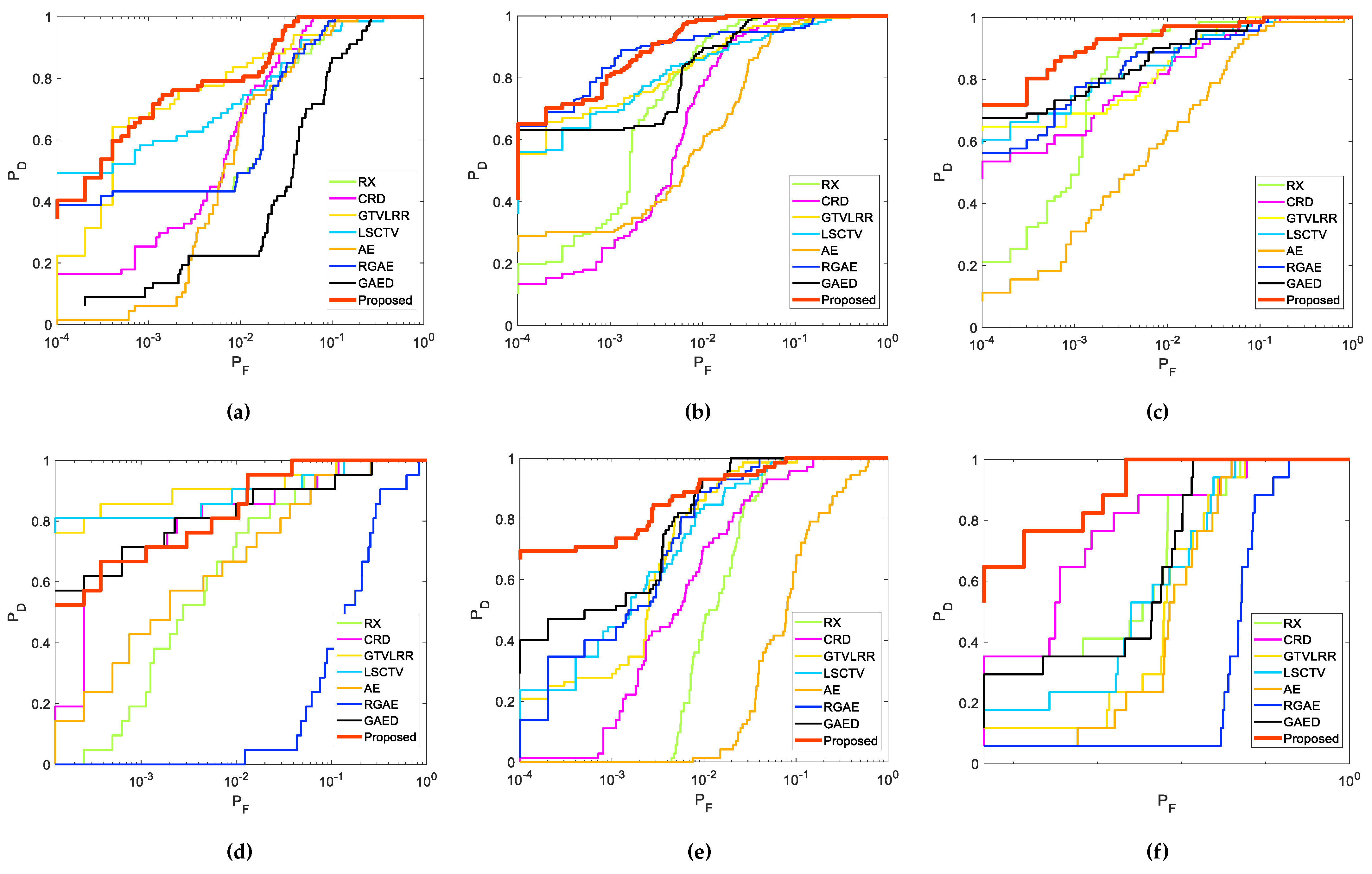
Figure 19 plots the ROC curves for the six datasets based on the eight anomaly detectors. It can be observed that the ROC curves of the proposed method are located in the top left corner for most of the datasets. It should be note that although the proposed method is just higher than others in a small range visually for the fourth dataset (HYDICE), it actually holds an advantage over a large range by virtue of the logarithmic scale of abscissa. In addition, the AU C D , F values based on these eight anomaly detectors are listed in Table 7. It is obvious that the proposed method is superior to other competitors.

4.3. Summary

The experiments on two synthetic datasets and six real datasets adequately demonstrated the superiority of the proposed method. The three primary benefits of the method are briefly summarized as follows:
(1)
Effectiveness: Owing to the unique long-range self-attention mechanism of TR, the spatial similarity among pixels and the spectral similarity among bands are characterized precisely by the 3DTR network. This strategy is more effective for reconstructing a background than AE-based detectors when considering spatial properties. To obtain a better reconstruction result for a background, coarse pre-detection is executed to avoid the contamination of anomalies. In addition, the proposed patch-generation method alleviates the contamination of weakly relevant pixels in the reconstruction procedure. The experimental results demonstrated that the proposed method is able to identify all anomalies effectively;
(2)
Convenience in Parameter Settings: There is only one loss item in the loss function, and thus no trade-off parameters need to be set. In addition, an analysis of the parameter settings indicates that the detection accuracies of the proposed method are insensitive to changes in the pre-detection parameter N a and the patch-generation parameter N P over a relatively wide range. Moreover, N a and N P are fixed throughout all the experiments, and satisfactory anomaly detection results are still achieved;
(3)
Robustness to Noise: For a full consideration of the spatial similarity among pixels and the spectral similarity among bands by the proposed method, random noise is effectively eliminated by characterizing the spatial properties. Specifically, the experimental results on two group synthetic datasets with different anomalous abundances and different levels of noise demonstrate that the proposed method is robust.
Additionally, the prominent disadvantage of the proposed method is the relatively high training time, which is due to the fact that the proposed method trains the network by patches of pixels in several epochs. However, it is worth noting that the test time is still within the acceptable range listed in Table 2, which indicates that the 3DTR has real application value after being trained in advance.

5. Conclusions

In this paper, a novel background reconstruction framework via 3D-Transformer network has been proposed for the hyperspectral anomaly detection. The effectiveness and robustness of the proposed method have been adequately demonstrated by the experimental results on both synthetic and real hyperspectral datasets. Specifically, two ablation experiments comprehensively confirmed the contribution of each component in the proposed method. Moreover, the parameter experiments demonstrated that the detection results of the proposed method are relatively insensitive to the choices of the involved parameters. Furthermore, the generalization ability of the proposed 3DTR network was verified by the generalization experiment. Last but not least, the comparison experiments with other SOTA competitors on both synthetic and real hyperspectral datasets adequately demonstrated that most of the anomalies were detected by the proposed method with relatively few false alarms.
Although the test time of the proposed method is within an acceptable range, the experimental results indicate that its training time is relatively high; the training time can be significantly reduced by replacing the CPU with GPU in the running of codes.

Author Contributions

Conceptualization, Z.W. and B.W.; methodology, Z.W. and B.W.; software, Z.W.; validation, Z.W. and B.W.; formal analysis, Z.W. and B.W.; investigation, Z.W.; resources, B.W.; data curation, Z.W.; writing—original draft preparation, Z.W. and B.W.; writing—review and editing, Z.W. and B.W.; visualization, Z.W.; supervision, B.W.; project administration, B.W.; funding acquisition, B.W. All authors have read and agreed to the published version of the manuscript.

Funding

This research was funded by the National Natural Science Foundation of China, grant number 61971141 and the National Key Research and Development Program of China, grant number 2022YFB3903404.

Institutional Review Board Statement

Not applicable.

Data Availability Statement

The data presented in this study are available on request from the corresponding author.

Conflicts of Interest

The authors declare no conflict of interest.

References

  1. Bioucas-Dias, J.M.; Plaza, A.; Camps-Valls, G.; Scheunders, P.; Nasrabadi, N.; Chanussot, J. Hyperspectral remote sensing data analysis and future challenges. IEEE Geosci. Remote Sens. Mag. 2013, 1, 6–36. [Google Scholar] [CrossRef]
  2. Ghamisi, P.; Yokoya, N.; Li, J.; Liao, W.; Liu, S.; Plaza, J.; Rasti, B.; Plaza, A. Advances in hyperspectral image and signal processing: A comprehensive overview of the state of the art. IEEE Geosci. Remote Sens. Mag. 2017, 5, 37–78. [Google Scholar] [CrossRef]
  3. Liu, L.; Wang, Y.; Peng, J.; Zhang, L.; Zhang, B.; Cao, Y. Latent relationship guided stacked sparse autoencoder for hyperspectral imagery classification. IEEE Trans. Geosci. Remote Sens. 2020, 58, 3711–3725. [Google Scholar] [CrossRef]
  4. Wang, X.; Tan, K.; Du, Q.; Chen, Y.; Du, P. CVA2E: A conditional variational autoencoder with an adversarial training process for hyperspectral imagery classification. IEEE Trans. Geosci. Remote Sens. 2020, 58, 5676–5692. [Google Scholar] [CrossRef]
  5. Sun, L.; Wu, F.; Zhan, T.; Liu, W.; Wang, J.; Jeon, B. Weighted nonlocal low-rank tensor decomposition method for sparse unmixing of hyperspectral images. IEEE J. Sel. Top. Appl. Earth Observ. Remote Sens. 2020, 13, 1174–1188. [Google Scholar] [CrossRef]
  6. Nasrabadi, N.M. Hyperspectral target detection: An overview of current and future challenges. IEEE Signal Process. Mag. 2014, 31, 34–44. [Google Scholar] [CrossRef]
  7. Xu, Y.; Zhang, L.; Du, B.; Zhang, L. Hyperspectral anomaly detection based on machine learning: An overview. IEEE J. Sel. Top. Appl. Earth Observ. Remote Sens. 2022, 15, 3351–3364. [Google Scholar] [CrossRef]
  8. He, C.; Sun, L.; Huang, W.; Zhang, J.; Zheng, Y.; Jeon, B. TSLRLN: Tensor subspace low-rank learning with non-local prior for hyperspectral image mixed denoising. Signal Process. 2021, 184, 108060. [Google Scholar] [CrossRef]
  9. Sun, L.; He, C.; Zheng, Y.; Tang, S. SLRL4D: Joint restoration of subspace low-rank learning and non-local 4-D transform filtering for hyperspectral image. Remote Sens. 2020, 12, 2979. [Google Scholar] [CrossRef]
  10. Dao, M.; Kwan, C.; Ayhan, B.; Tran, T.D. Burn scar detection using cloudy MODIS images via low-rank and sparsity-based models. In Proceedings of the 2016 IEEE Global Conference on Signal and Information Processing (GlobalSIP), Washington, DC, USA, 7–9 December 2016; pp. 177–181. [Google Scholar]
  11. Huang, Z.; Li, S. From difference to similarity: A manifold ranking based hyperspectral anomaly detection framework. IEEE Trans. Geosci. Remote Sens. 2019, 57, 8118–8130. [Google Scholar] [CrossRef]
  12. Gagnon, M.-A.; Tremblay, P.; Savary, S.; Lagueux, P.; Chamberland, M. Standoff thermal hyperspectral imaging for flare and smokestack characterization in industrial environments. In Proceedings of the 2013 5th Workshop on Hyperspectral Image and Signal Processing: Evolution in Remote Sensing (WHISPERS), Gainesville, FL, USA, 26–28 June 2013; pp. 1–4. [Google Scholar]
  13. Kruse, F.A.; Boardman, J.W.; Huntington, J.F. Comparison of airborne hyperspectral data and EO-1 Hyperion for mineral mapping. IEEE Trans. Geosci. Remote Sens. 2003, 41, 1388–1400. [Google Scholar] [CrossRef]
  14. Wang, J.; Zhang, L.; Tong, Q.; Sun, X. The spectral crust project—Research on new mineral exploration technology. In Proceedings of the 2012 4th Workshop on Hyperspectral Image and Signal Processing: Evolution in Remote Sensing (WHISPERS), Shanghai, China, 4–7 June 2012; pp. 1–4. [Google Scholar]
  15. Eismann, M.T.; Stocker, A.D.; Nasrabadi, N.M. Automated hyperspectral cueing for civilian search and rescue. Proc. IEEE 2009, 97, 1031–1055. [Google Scholar] [CrossRef]
  16. Antson, L.; Vandenhoeke, A.; Shimoni, M.; Hamesse, C.; Luong, H. Detection and tracking of search and rescue personnel under hindered light conditions using hyperspectral imaging. In Proceedings of the 2022 12th Workshop on Hyperspectral Imaging and Signal Processing: Evolution in Remote Sensing (WHISPERS), Rome, Italy, 13–16 September 2022; pp. 1–6. [Google Scholar]
  17. Ardouin, J.-P.; Lévesque, J.; Rea, T.A. A demonstration of hyperspectral image exploitation for military applications. In Proceedings of the 2007 10th International Conference on Information Fusion, Quebec, QC, Canada, 9–12 July 2007; pp. 1–8. [Google Scholar]
  18. Racek, F.; Barta, V. Spectrally based method of target detection in acquisition system of general fire control system. In Proceedings of the 2017 International Conference on Military Technologies (ICMT), Brno, Czech Republic, 31 May–2 June 2017; pp. 22–26. [Google Scholar]
  19. Reed, I.S.; Yu, X. Adaptive multiple-band CFAR detection of an optical pattern with unknown spectral distribution. IEEE Trans. Acoust. Speech Signal Process. 1990, 38, 1760–1770. [Google Scholar] [CrossRef]
  20. Li, W.; Du, Q. Collaborative representation for hyperspectral anomaly detection. IEEE Trans. Geosci. Remote Sens. 2015, 53, 1463–1474. [Google Scholar] [CrossRef]
  21. Candès, E.J.; Li, X.; Ma, Y.; Wright, J. Robust principal component analysis? J. ACM 2011, 58, 11. [Google Scholar] [CrossRef]
  22. Wang, W.; Li, S.; Qi, H.; Ayhan, B.; Kwan, C.; Vance, S. Identify anomaly component by sparsity and low rank. In Proceedings of the 2015 7th Workshop on Hyperspectral Image and Signal Processing: Evolution in Remote Sensing (WHISPERS), Tokyo, Japan, 2–5 June 2015; pp. 1–4. [Google Scholar]
  23. Liu, G.; Lin, Z.; Yan, S.; Sun, J.; Yu, Y.; Ma, Y. Robust recovery of subspace structures by low-rank representation. IEEE Trans. Pattern Anal. Mach. Intell. 2013, 35, 171–184. [Google Scholar] [CrossRef]
  24. Xu, Y.; Wu, Z.; Li, J.; Plaza, A.; Wei, Z. Anomaly detection in hyperspectral images based on low-rank and sparse representation. IEEE Trans. Geosci. Remote Sens. 2016, 54, 1990–2000. [Google Scholar] [CrossRef]
  25. Cheng, T.; Wang, B. Graph and total variation regularized lowrank representation for hyperspectral anomaly detection. IEEE Trans. Geosci. Remote Sens. 2020, 58, 391–406. [Google Scholar] [CrossRef]
  26. Feng, R.; Li, H.; Wang, L.; Zhong, Y.; Zhang, L.; Zeng, T. Local spatial constraint and total variation for hyperspectral anomaly detection. IEEE Trans. Geosci. Remote Sens. 2022, 60, 1–16. [Google Scholar] [CrossRef]
  27. Hinton, G.E.; Zemel, R.S. Autoencoders, minimum description length and Helmholtz free energy. Adv. Neural Inf. Process. Syst. 1994, 6, 3–10. [Google Scholar]
  28. Jiang, T.; Li, Y.; Xie, W.; Du, Q. Discriminative Reconstruction Constrained Generative Adversarial Network for Hyperspectral Anomaly Detection. IEEE Trans. Geosci. Remote Sens. 2020, 58, 4666–4679. [Google Scholar] [CrossRef]
  29. Goodfellow, I.; Pouget-Abadie, J.; Mirza, M.; Xu, B.; Warde-Farley, D.; Ozair, S.; Courville, A.; Bengio, Y. Generative adversarial nets. Adv. Neural Inf. Process. Syst. 2014, 2672–2680. [Google Scholar] [CrossRef]
  30. Fan, G.; Ma, Y.; Mei, X.; Fan, F.; Huang, J.; Ma, J. Hyperspectral anomaly detection with robust graph autoencoders. IEEE Trans. Geosci. Remote Sens. 2022, 60, 1–14. [Google Scholar] [CrossRef]
  31. Jiang, K.; Xie, W.; Li, Y.; Lei, J.; He, G.; Du, Q. Semisupervised spectral learning with generative adversarial network for hyperspectral anomaly detection. IEEE Trans. Geosci. Remote Sens. 2020, 58, 5224–5236. [Google Scholar] [CrossRef]
  32. Xiang, P.; Ali, S.; Jung, S.K.; Zhou, H. Hyperspectral anomaly detection with guided autoencoder. IEEE Trans. Geosci. Remote Sens. 2022, 60, 1–18. [Google Scholar] [CrossRef]
  33. Vaswani, A.; Shazeer, N.; Parmar, N.; Uszkoreit, J.; Jones, L.; Gomez, A.N.; Kaiser, Ł.; Polosukhin, I. Attention is all you need. Adv. Neural Inf. Process. Syst. 2017, 30, 5998–6008. [Google Scholar]
  34. Sun, L.; Zhao, G.; Zheng, Y.; Wu, Z. Spectral–spatial feature tokenization transformer for hyperspectral image classification. IEEE Trans. Geosci. Remote Sens. 2022, 60, 1–14. [Google Scholar] [CrossRef]
  35. Hu, X.; Yang, W.; Wen, H.; Liu, Y.; Peng, Y. A lightweight 1-D convolution augmented transformer with metric learning for hyperspectral image classification. Sensors 2021, 21, 1751. [Google Scholar] [CrossRef]
  36. He, X.; Chen, Y.; Lin, Z. Spatial-spectral transformer for hyperspectral image classification. Remote Sens. 2021, 13, 498. [Google Scholar] [CrossRef]
  37. Wang, Y.; Hong, D.; Sha, J.; Gao, L.; Liu, L.; Zhang, Y.; Rong, X. Spectral–spatial–temporal transformers for hyperspectral image change detection. IEEE Trans. Geosci. Remote Sens. 2022, 60, 1–14. [Google Scholar] [CrossRef]
  38. Xiao, S.; Zhang, T.; Xu, Z.; Qu, J.; Hou, S.; Dong, W. Anomaly detection of hyperspectral images based on transformer with spatial–spectral dual-window mask. IEEE J. Sel. Top. Appl. Earth Observ. Remote Sens. 2023, 16, 1414–1426. [Google Scholar]
  39. Li, K.; Wang, S.; Zhang, X.; Xu, Y.; Xu, W.; Tu, Z. Pose recognition with cascade transformers. CVPR 2021, 1944–1953. [Google Scholar] [CrossRef]
  40. Zheng, S.; Lu, J.; Zhao, H.; Zhu, X.; Luo, Z.; Wang, Y.; Fu, Y.; Feng, J.; Xiang, T.; Torr, P.; et al. Rethinking semantic segmentation from a sequence-to-sequence perspective with transformers. CVPR 2021, 6877–6886. [Google Scholar] [CrossRef]
  41. He, X.; Zhou, Y.; Zhao, J.; Zhang, D.; Yao, R.; Xue, Y. Swin transformer embedding UNet for remote sensing image semantic segmentation. IEEE Trans. Geosci. Remote Sens. 2022, 60, 1–15. [Google Scholar] [CrossRef]
  42. Dai, X.; Chen, Y.; Yang, J.; Zhang, P.; Yuan, L.; Zhang, L. Dynamic DETR: End-to-end object detection with dynamic attention. ICCV 2021, 2968–2977. [Google Scholar] [CrossRef]
  43. Rao, W.; Gao, L.; Qu, Y.; Sun, X.; Zhang, B.; Chanussot, J. Siamese transformer network for hyperspectral image target detection. IEEE Trans. Geosci. Remote Sens. 2022, 60, 1–19. [Google Scholar] [CrossRef]
  44. Dosovitskiy, A.; Beyer, L.; Kolesnikov, A.; Weissenborn, D.; Zhai, X.; Unterthiner, T.; Dehghani, M.; Minderer, M.; Heigold, G.; Gelly, S.; et al. An image is worth 16x16 words: Transformers for image recognition at scale. arXiv 2020, arXiv:2010.11929. [Google Scholar] [CrossRef]
  45. Zhong, Z.; Li, Y.; Ma, L.; Li, J.; Zheng, W. Spectral–spatial transformer network for hyperspectral image classification: A factorized architecture search framework. IEEE Trans. Geosci. Remote Sens. 2022, 60, 1–15. [Google Scholar] [CrossRef]
  46. Chang, C.-I. An effective evaluation tool for hyperspectral target detection: 3D receiver operating characteristic curve analysis. IEEE Trans. Geosci. Remote Sens. 2021, 59, 5131–5153. [Google Scholar] [CrossRef]
  47. Schweizer, S.M.; Moura, J.M.F. Efficient detection in hyperspectral imagery. IEEE Trans. Image Process. 2001, 10, 584–597. [Google Scholar]
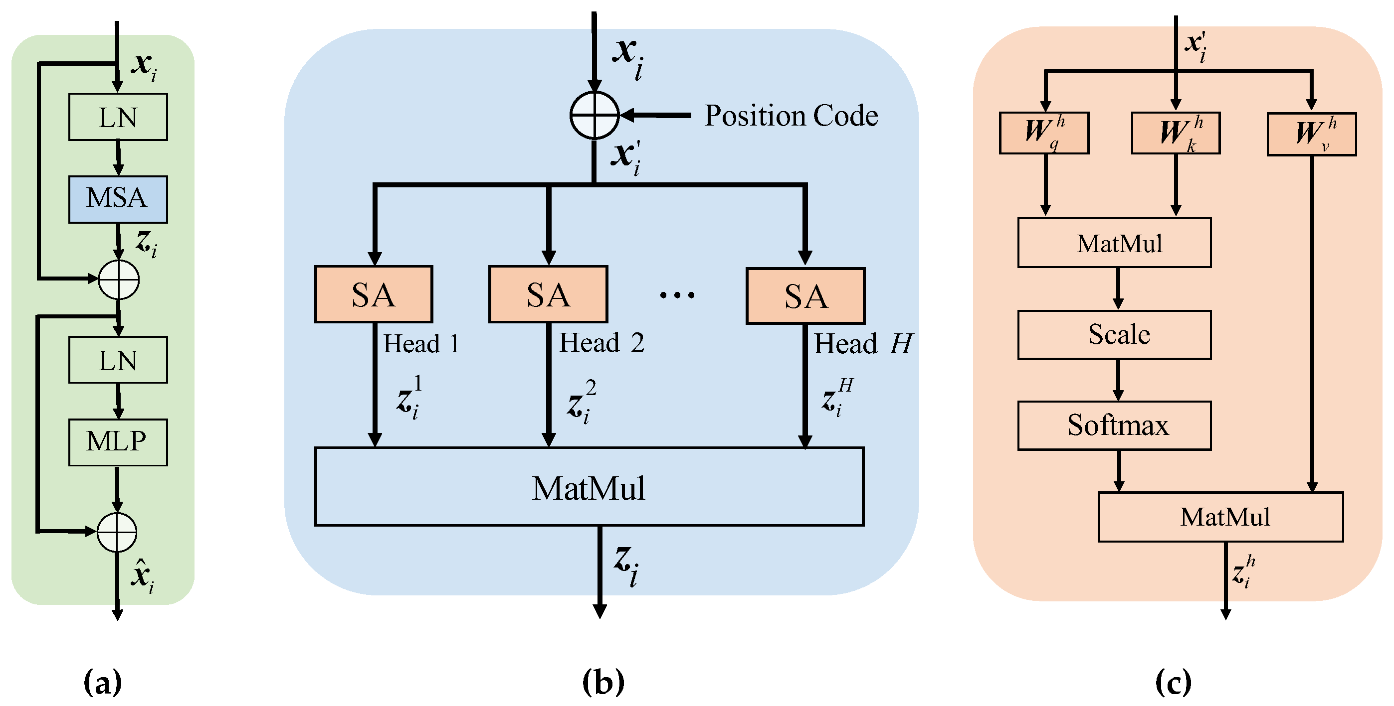
Figure 1. The flowcharts of the traditional transformer module: (a) the overall structure of the traditional transformer module; (b) the multi-head self-attention (MSA) block; and (c) the h-th self-attention (SA) block.
Remotesensing 15 04592 g001
Figure 2. Overview of the proposed method for hyperspectral anomaly detection.
Remotesensing 15 04592 g002
Figure 3. Difference between traditional and proposed patch-generating methods: (a) the patch generated by the traditional method in the sketch map; (b) the patch generated by the proposed method in the sketch map; (c) the patch generated by the proposed method in the real HSIs; and (d) only highlighted similar pixels are picked out.
Remotesensing 15 04592 g003
Figure 4. The first synthetic hyperspectral dataset: (a) whole pseudocolor image; (b) the selected anomaly spectra t from an airplane in the pristine whole scene; (c) pseudocolor image of the first synthetic dataset; and (d) ground truth map.
Remotesensing 15 04592 g004
Figure 5. Anomaly detection maps obtained by all the anomaly detectors on the first synthetic dataset.
Remotesensing 15 04592 g005
Figure 6. 3D ROC curves of all the anomaly detectors on the first synthetic dataset: (a) 3D ROC curves; (b) 2 D RO C D , F curves; (c) 2 D RO C D , τ curves; and (d) 2 D RO C F , τ curves.
Remotesensing 15 04592 g006
Figure 7. ROC curves of all anomaly detectors for the first synthetic dataset with different levels of noise: (a) 30 dB; (b) 25 dB; and (c) 20 dB.
Remotesensing 15 04592 g007
Figure 8. Anomaly detection maps obtained by the proposed method after removing different components. Cases: (a) C1; (b) C2; (c) C3; and (d) C4.
Remotesensing 15 04592 g008
Figure 9. ROC curves of the proposed method after removing different components.
Remotesensing 15 04592 g009
Figure 10. Flowcharts of different combination modes. Cases: (a) M1; (b) M2; (c) M3; and (d) M4.
Remotesensing 15 04592 g010
Figure 11. Anomaly detection maps obtained by the proposed method on different combination modes: cases (a) M1; (b) M2; (c) M3; and (d) M4.
Remotesensing 15 04592 g011
Figure 12. ROC curves of the proposed method on different combination modes.
Remotesensing 15 04592 g012
Figure 13. Influences of involved parameters on the detection accuracy of the proposed method: (a) pre-detection parameter N a ; and (b) patch-generation parameter N p .
Remotesensing 15 04592 g013
Figure 14. The generalization evaluation of the proposed 3DTR network: (a) the segmentation of the training set and the validation set; (b) the anomaly detection map of the testing set (AUC = 0.9991); and (c) the anomaly detection map of the validation set (AUC = 1.0000).
Remotesensing 15 04592 g014
Figure 15. Loss curves of the 3DTR network on the training set and validation set.
Remotesensing 15 04592 g015
Figure 16. ROC curves of all anomaly detectors for the second synthetic dataset with different levels of noise: (a) 30 dB; (b) 25 dB; and (c) 20 dB.
Remotesensing 15 04592 g016
Figure 17. The pseudocolor images (left) and the corresponding ground truth maps (right) of six real hyperspectral datasets: (a) Texas Coast-1; (b) Texas Coast-2; (c) Pavia; (d) HYDICE; (e) San Diego; and (f) Hyperion.
Remotesensing 15 04592 g017
Figure 18. Anomaly detection maps of all detectors on the six real hyperspectral datasets.
Remotesensing 15 04592 g018
Figure 19. ROC curves of all anomaly detectors on the six real hyperspectral datasets: (a) Texas Coast-1; (b) Texas Coast-2; (c) Pavia; (d) HYDICE; (e) San Diego; and (f) Hyperion.
Remotesensing 15 04592 g019
Table 1. Detailed network configurations of the proposed 3DTR.
NetworkParameterValue
Spatial TransformerMSAHead5
MLPInput ChannelL
Hidden Channel10
Spectral TransformerMSAHead5
MLPInput Channel121
Hidden Channel10
Table 2. AUC values and running times of all the detectors on the synthetic datasets.
AlgorithmAUC(D, F)AUC(D, τ)AUC(F, τ)AUCTDAUCBSAUCSNPRAUCTDBSAUCODTraining
Time (s)
Test
Time (s)
RX0.99120.42630.01531.41760.976027.92350.41111.40230.2168
CRD0.96860.38410.03751.35270.931110.25620.34661.31523.2920
GTVLRR0.99690.54960.04461.54650.952312.33360.50511.5020101.5662
LSC-TV0.99540.53550.03001.53090.965417.84930.50551.5009405.3491
AE0.82860.15430.06800.98290.76062.26880.08630.91498.55870.0865
RGAE0.95880.35070.02821.30950.930712.44510.32251.281381.51060.0679
GAED0.99780.27070.00661.26860.991241.01010.26411.262018.88710.0630
Proposed0.99930.55740.05101.55660.94339.95410.50641.5056159.16809.7920
Table 3. AUC values (mean ± std) of all anomaly detectors for the first synthetic dataset with different levels of noise (20 replicates for each noise level).
AlgorithmRXCRDGTVLRRLSCTVAERGAEGAEDProposed
30 dB0.9908 ±
0.0017
0.9628 ±
0.0250
0.9952 ±
0.0029
0.9868 ±
0.0031
0.8744 ±
0.0435
0.9578 ±
0.0028
0.9957 ±
0.0022
0.9987 ±
0.0005
25 dB0.9810 ±
0.0035
0.9450 ±
0.0314
0.9949 ±
0.0030
0.9814 ±
0.0043
0.8623 ±
0.0443
0.9564 ±
0.0040
0.9954 ±
0.0026
0.9975 ±
0.0016
20 dB0.9569 ±
0.0269
0.9348 ±
0.0340
0.9932 ±
0.0042
0.9762 ±
0.0091
0.8534 ±
0.0494
0.9546 ±
0.0082
0.9930 ±
0.0045
0.9944 ±
0.0039
Table 4. Detail settings of different cases in two ablation experiments.
Ablation CasesDetails
Ablation on Different ComponentsC1Only spatial TR module with the proposed patch-generating method
C2Only spectral TR module with the proposed patch-generating method
C3The proposed 3DTR network with a single window to generate patches
C4The proposed 3DTR network with the proposed patch-generating method
Ablation on Different Combination ModesM1Add the respective detection results of two TR modules
M2Multiply the respective detection results of two TR modules
M3Combine two TR modules in parallel anatomically
M4Combine two TR modules in series anatomically, namely the proposed 3DTR network
Table 5. AUC values (mean ± std) of all anomaly detectors for the second synthetic dataset with different levels of noise (20 replicates for each level of noise).
AlgorithmRXCRDGTVLRRLSCTVAERGAEGAEDProposed
30 dB0.9846 ±
0.0041
0.9409 ±
0.0338
0.9931 ±
0.0035
0.9408 ±
0.0082
0.8318 ±
0.0571
0.9133 ±
0.0054
0.9875 ±
0.0043
0.9946 ±
0.0019
25 dB0.9760 ±
0.0073
0.9291 ±
0.0370
0.9835 ±
0.0086
0.9317 ±
0.0092
0.8205 ±
0.0588
0.9102 ±
0.0058
0.9823 ±
0.0078
0.9939 ±
0.0038
20 dB0.9464 ±
0.0281
0.9199 ±
0.0507
0.9710 ±
0.0112
0.9309 ±
0.0125
0.7946 ±
0.0869
0.9072 ±
0.0068
0.9792 ±
0.0082
0.9912 ±
0.0066
Table 6. The image characteristics of the six real hyperspectral datasets.
DatasetsSizeBandsNumber of AnomaliesAnomaly TypesWindow Sizes of CRD
Texas Coast-1100 × 10020467 (0.67%)Buildings(3, 7)
Texas Coast-2100 × 100207155 (1.55%)Buildings(3, 15)
Pavia100 × 10010271 (0.71%)Vehicles(3, 13)
HYDICE80 × 10017421 (0.26%)Buildings and Vehicles(3, 9)
San Diego100 × 10018672 (0.72%)Airplanes(3, 7)
Hyperion150 × 15015517 (0.08%)Storage
Silo
(3, 11)
Table 7. AUC values of all anomaly detectors on the six real hyperspectral datasets.
AlgorithmRXCRDGTVLRRLSC-TVAERGAEGAEDProposed
Texas Coast-10.98100.98830.99050.98180.98090.98210.99090.9946
Texas Coast-20.99640.99180.99270.98870.98190.99260.99590.9991
Pavia0.99130.99170.99480.99370.97120.99270.99480.9972
HYDICE0.98600.98920.99300.99060.97620.79490.98080.9959
San Diego0.98270.98330.99450.99290.87550.99400.99510.9958
Hyperion0.99250.99440.98890.99080.98800.94080.99490.9996
Disclaimer/Publisher’s Note: The statements, opinions and data contained in all publications are solely those of the individual author(s) and contributor(s) and not of MDPI and/or the editor(s). MDPI and/or the editor(s) disclaim responsibility for any injury to people or property resulting from any ideas, methods, instructions or products referred to in the content.