Abstract
Climate change has significantly influenced water resource patterns in arid regions. Applying effective water-saving measures to improve irrigation efficiency and evaluate their future water-saving capabilities is crucial for ensuring the sustainable development of irrigation agriculture. Based on the daily meteorological data from 15 global climate models (GCMs) in the sixth phase of the Coupled Model Intercomparison Project (CMIP6), this study used the AquaCrop model to perform high-resolution (0.1° × 0.1°) grid simulations of cotton yields and irrigation requirements. The study also investigated the ability of film-mulched drip irrigation (FMDI) to improve future irrigation efficiency under two shared socio-economic pathways (SSP245 and SSP585) in the Tarim River Basin (TRB), Central Asia, from 2025 to 2100. The results showed that the cotton yield and irrigation water productivity (WPI) in the TRB exhibited an upward trend of 13.82 kg/ha/decade (80.68 kg/ha/decade) and 0.015 kg/m3/decade (0.068 kg/m3/decade), respectively, during the study period. The cotton yield and WPI were higher in the northern, northwestern plains, and northeastern intermountain basin areas, where they reach over 4000 kg/ha and 0.8 kg/m3/decade. However, the cotton yield and WPI were lower in the southwestern part of the study area. Therefore, large-scale cotton production was not recommended there. Furthermore, compared to flood irrigation, the use of FMDI can, on average, improve the WPI by approx. 25% and reduce irrigation water requirements by more than 550 m3/ha. Therefore, using FMDI can save a substantial amount of irrigation water in cotton production, which is beneficial for improving irrigation efficiency and ensuring the future stable production of cotton in the TRB. The research results provide a scientific reference for the efficient utilization and management of water resources for cotton production in the TRB and in similar arid regions elsewhere in the world.
1. Introduction
The continuous increase in global temperature and atmospheric carbon dioxide (CO2) concentrations has received widespread attention for its impact on agricultural production [1,2,3]. In arid regions, which account for 41% of the global land area, the warming trend is significantly higher than the global average, making these regions more sensitive to climate change [4,5]. Precipitation patterns in arid zones are also affected by the warming climate, increasing the frequency of extreme rainfall, accelerating glacier melting, and changing the usage patterns of existing water resources [6,7]. These changes pose a serious risk to irrigation agriculture, where water resources are the primary limiting factor [8].
The Tarim River Basin (TRB) in Central Asia has a fragile ecosystem that is highly sensitive to climate change. In recent decades, changes in water storage and accelerated glacier melting have emerged in the TRB, which have disrupted water resource allocation in the region [9]. Despite its arid environment, the TRB is an important cotton production base in China and one of the major cotton producing areas in the world. However, cotton is a water-intensive crop that requires significant irrigation during production, which exacerbates the water resource burden [10]. Therefore, it is crucial to identify effective adaptation measures to mitigate the more severe water constraints that cotton production in the TRB may face under climate change [11].
In previous studies, agricultural water-saving measures have been employed to improve irrigation efficiency, showing they provide an effective means to alleviate water resource stress for irrigated agriculture in arid and semi-arid regions [12]. A meta-analysis of drip irrigation demonstrated that improved irrigation methods can significantly enhance the yield, water productivity, and nitrogen use efficiency, leading to water and fertilizer conservation [13]. Ding, et al. [14] simulated the effects of different levels of deficit irrigation on crop yield using the DSSAT crop model. The results indicated that the crop yield and water productivity were significantly enhanced under deficit irrigation. Feng, et al. [15] showed through field experiments that mulching film improved soil moisture and heat conditions in arid areas, promoting crop growth. Although the above-mentioned measures have shown significant water-saving capabilities, deficit irrigation usually requires adjusting irrigation plans by considering factors such as irrigation methods, climate conditions, soil properties, etc. Hence, various difficulties remain in implementing these measures in practical applications [16]. One approach that combines drip irrigation and mulching film is film mulching drip irrigation (FMDI). FMDI not only decreases losses during irrigation, but also reduces water waste due to soil evaporation during crop growth, thereby further improving the water-saving capacity [17,18]. In addition, FMDI can improve soil temperature conditions, ensuring that crops have the necessary heat during their early growth stages or the wheat green-up period [19,20]. For widespread saline–alkali land in arid regions, FMDI can inhibit salt accumulation in the root zone, alleviating the salt stress faced by crops during growth [21,22]. Due to FMDI’s numerous advantages and excellent water-saving abilities, several locations across the TRB have promoted and applied the technique, including cotton production [23]. However, under the threat of future climate change, further research is needed to evaluate whether FMDI’s water-saving abilities will be challenged or whether the method will continue to serve as an effective measure for saving agricultural water.
Process-based crop models, such as DSSAT, EPIC, APSIM, and AquaCrop, are increasingly being used as low-cost and efficient methods to evaluate the impact of climate factors and irrigation management on crop growth and yield formation [23,24]. Since most crop models can simulate crop growth changes caused by changes in CO2 concentrations during the simulation process, they have also been used in recent years to assess the impact of climate change on agricultural production [2,25]. AquaCrop is a water-driven model that can be used to evaluate crop productivity related to the water supply and agronomic management. It is often used to simulate crop responses and soil moisture changes under different irrigation scenarios [23,26]. This kind of application uses field experiments and site-scale simulations, with model parameters that are mostly obtained through experimental observations [23]. However, when the focus of a study is the analysis of crop irrigation water demand at the basin scale, site-scale simulations are often unable to meet the research needs. Therefore, to satisfy the demand for large-scale simulations in climate change research in recent years, scientists have developed global gridded crop models and corresponding input datasets [27,28]. Unfortunately, the spatial resolution of these models is 0.5°, which is somewhat rough and inadequate when applied at the basin scale. Achieving higher resolution gridded simulations and creating corresponding gridded input data are two important problems that crop modelers need to solve.
To that end, the present study quantified the water-saving abilities of FMDI in the TRB under future climate change. Based mainly on observational data and the data from 15 global climate models (GCMs), the AquaCrop model was used to simulate the cotton yield, irrigation requirements, and soil evaporation at a resolution of 0.1° for two shared socio-economic pathways (SSPs) and two irrigation conditions. The SSPs were SSP245 and SSP585, and the conditions were flood irrigation (FI) and FMDI in the TRB from 2025 to 2100 at the basin scale. According to the simulation results, the following aspects were analyzed: (1) the spatiotemporal changes in future cotton yield in the TRB under a changing climate; (2) the spatiotemporal changes in future cotton irrigation water productivity (WPI); and (3) the FMDI’s capacity to improve future cotton WPI. This study provides important scientific evidence for the sustainable development of irrigation agriculture and for alleviating pressure on agricultural water use in the TRB. It also offers decision-making references for future agricultural layout adjustments and watershed water resources planning.
2. Study Area and Data
2.1. Study Area
The Tarim River Basin is located in the hinterland of the Eurasian continent (34.6°–43.4°N, 73.1°–90.3°E) (Figure 1). It is surrounded by high mountains, has few water bodies other than rivers, and is far from the ocean. These factors give the TRB an extremely arid climate, with an annual precipitation of less than 50 mm and the potential evaporation exceeding 3000 mm. The center of the basin is dominated by the world’s second largest mobile desert, the Taklimakan Desert [29]. The croplands in the basin are mainly distributed along the rivers and piedmont (foothills) plains, and almost all of them are irrigated agriculture. Due to the region’s paucity of large water bodies, glacier and snow meltwater are important sources of irrigation water in the TRB.
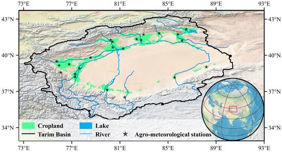
Figure 1.
Geographical location of the study area, distribution of croplands and stations, and topography of the study area. The base map was derived from the Natural Earth dataset, which is available at naturalearthdata.com, accessed on 10 September 2020.
2.2. Data
The historical climate data and phenological observation data used for the model calibration and validation in the study were obtained from 23 agro-meteorological stations in the TRB. The simulated climate data for the future period were derived from the daily data of 15 GCMs under two shared socio-economic pathways (SSP245 and SSP585) in the sixth phase of the Coupled Model Intercomparison Project (CMIP6) (Table S1). The SSP is a prediction of the future climate that takes into account a variety of factors, including the rate of greenhouse gas emissions, natural forcing, and socio-economic changes such as the population, urban development, and emission reduction policies. Among them, SSP245 represents CO2 emissions hovering around the current levels before starting to decline in the middle of the century, but not reaching net zero by 2100. This represents a “middle path” for climate change. SSP585 represents a baseline scenario in which CO2 emissions continue to increase without policy intervention, which is the worst-case scenario. Under the two scenarios, warming by the end of the century would be 2.7 °C and 4.4 °C, respectively.
Since the different GCM data have different resolutions, and numerous studies have indicated that there are certain errors between the GCMs and the historical observation data [30], the present study applied the ISIMIP3BASD method to bias-correct and downscale the data from the 15 GCMs [31], and then unify the data into a resolution of 0.1°. The reference evapotranspiration (ET0) required by the AquaCrop model for both the historical and future periods was calculated according to the “Food and Agriculture Organization (FAO)” Irrigation and Drainage Paper 56 [32].
The soil parameters required for the model were from the Harmonized World Soil Database (HWSD) [33], with an original resolution of 1 km (30 arc seconds × 30 arc seconds). The study used the soil parameters at the 0.1° grid center as the input data for the gridded simulation and resampled the soil data to a 0.1° resolution. The crop phenological parameters for the future period were based on the median observation data for each phenological period as the model inputs. To make the simulation results more accurate, the study calibrated and validated the model using the statistical data on the county-level cotton yield, which was from the Xinjiang Statistical Yearbook [34]. The statistical data included the average county-level cotton production of 23 counties from 2016 to 2020. The spatial distribution of cropland was based on “China’s Multi-Period Land Use Land Cover Remote Sensing Monitoring Data Set” (CNLUCC). The dataset was based on Landsat remote sensing images from the United States as the main information source, and the land use/land cover thematic database was constructed via manual visual interpretation. In order to fully consider the possible planting areas of cotton in the future, we initially resampled the land use data for all the periods (1980 to 2020) in the CNLUCC into a uniform 0.1° grid. Then, the union set of cultivated land in all the periods was taken as the range of the grid simulation. The resampling was done in a conservative manner using the “xESMF” Python package. The CNLUCC data was from the Resource and Environment Science Data Center [35].
2.3. Methods
2.3.1. AquaCrop Model
The AquaCrop model was developed by the FAO to address food security and evaluate the impact of environmental and management measures on crop production [26]. It can simulate the achievable yield of herbaceous crops under different conditions using a daily time step and is particularly suitable for simulating the effects of water conditions on crops. Currently, AquaCrop has been widely used to simulate many crops, such as maize [36], wheat [37], and cotton [23,38], and has achieved good simulation results. With the increasing demand for large-scale simulation, the FAO has also released a Python implementation of the model (AquaCrop-OSPy), which greatly improves its flexibility and computational efficiency [39].
A major advantage of AquaCrop over other crop models is that it not only requires fewer parameters, but the determination method of these parameters is simpler. To run the model, only a few explicit parameters and some mostly intuitive variables are needed [40]. Hence, the FAO’s AquaCrop offers simplicity, accuracy, and robustness. This ideal combination of characteristics means that the model can largely avoid the cumbersome process of preparing the input data when applied to the grid simulation.
AquaCrop separates the actual evapotranspiration () in agricultural fields into soil evaporation () and crop transpiration () (Equation (1)) and divides the final yield () into biomass () and the harvest index () (Equation (2)), which can be expressed as the following.
Additionally, the model distinguishes between soil evaporation and crop transpiration, which avoids the mixing effect of non-productive consumptive water. This is important because it provides the conditions for simulating the reduction in soil evaporation due to FMDI. It also simulates changes in soil evaporation caused by canopy shading during crop canopy development.
The crop biomass () is calculated using the crop transpiration () and water productivity normalized by the ET0 and CO2 concentration () [40]. The core formula can be expressed as the following.
where is the crop transpiration (in mm) and is the water productivity parameter (kg of biomass per m2 and per mm of cumulated water transpired over the time period in which the biomass is produced).
During the simulation process, Equation (3) was inserted into a set of additional model components to simulate the effects of other factors on crop growth. These factors included the soil water balance, climatic conditions, and management measures. The process allowed for the simulation of the final yields and irrigation requirements, along with other relevant information.
The present study used soil moisture variation as an irrigation trigger during the simulation process, where irrigation was triggered when the soil moisture decreased to 50% of the field capacity. The maximum irrigation amount per day was set at 25 mm.
The TRB’s FMDI consisted of two parts. The first part was the drip irrigation belt that plays the role of water supply and irrigation. Generally speaking, one drip irrigation belt was responsible for the irrigation of two rows of crops. The second part was the plastic film mulching that reduced evaporation and retained soil moisture. A combination of flat mulching and partially covered methods are usually employed. According to the research results from Kader et al. [18] and Li, et al. [41], this film mulching reduced approx. 70% of soil evaporation. Therefore, when simulating the FMDI conditions, we set the soil evaporation to 30% of the normal conditions, which changed the changing process of soil water and realized the simulation of the irrigation amounts and other aspects under the FMDI conditions.
All the crop simulations conducted in the present study, including the model calibration and validation, were based on AquaCrop-OSPy v2.2.
2.3.2. Model Calibration and Validation
Since there was no corresponding parameter calibration program for AquacCop, this study used an evolution strategy to estimate five parameters under the growing degree days (GDD) conditions at each site. The five parameters were the seeding density, maximum canopy cover (CCX), canopy growth coefficient (CGC), canopy decline coefficient (CDC), and harvest index (HI0) [42]. The other parameters required during calibration, such as the planting (GDD), emergence (GDD), HI_Start (GDD), flowering (GDD), and senescence (GDD), were derived from the actual phenological and meteorological data observed by the agricultural meteorological stations. The location distribution of the stations is shown in Figure 1. The parameters obtained from the actual observations and those generated by the evolutionary strategy together drove the AquaCrop model to generate the simulated cotton yield results. The root mean square error (RMSE) between the measured yield and the simulated yield was used as the fitness function for the evolutionary strategy.
Based on the experimental results, the average fitness of the population at each site could reach stability within 100 iterations. Therefore, the study set the number of iterations to 100 and used the group of parameters with the smallest RMSE in the last generation as the final calibration parameters for the corresponding site.
The range of crop parameters was determined based on the recommended range in the AquaCrop v6.1 reference manual and actual conditions [40], as shown in Table S2. The study used the data from 2016 to 2019 for the calibration and the data from 2020 for the validation. To evaluate the overall consistency between the simulated and observed yields for the 23 sites, the RMSE and the consistency index () were used. The evaluation results are shown in Table 1. The RMSE was calculated using the following formula (Equation (4)).
where is the observed yield, is the simulated yield of the model, and is the number of observations. The consistency index () was calculated according to the following formula (Equation (5)) [38].
where is the mean value of observed yields. The range of values was from 0 to 1, and the closer was to 1, the better the quality.

Table 1.
Statistical evaluation of the crop model simulated yield and observed yield.
2.3.3. Grid-Based Crop Simulation
According to the principle that “the more similar the geographical environment, the more similar the geographical features” [43,44], the crop parameters in the study area were expected to have certain similarities, since the sites shared similar natural and socio-economic conditions. Therefore, this study used a combination of spatial interpolation and cross-validation to address the issue of the grid input parameters that were lacking.
First, the interpolations were performed based on the observed phenological parameters and estimated crop parameters. Each interpolation used the data from the 22 stations, and the results were extracted from the non-interpolated station. The interpolation was repeated 23 times to obtain the interpolation results for all the stations. Next, the RMSE and were used to evaluate the 23 sets of actual and interpolated values to determine the optimal interpolation method for each parameter. Finally, the optimal interpolation method for each parameter was employed to generate the gridded parameters using the data from the 23 stations as the input.
The above method not only evaluated the accuracy of the interpolation results under different interpolation methods using cross-validation to determine whether the current interpolation method met the requirements [45]. It also allowed for the early selection of more suitable interpolation methods based on the spatial distribution patterns of the other factors that affected the parameters. This approach further improved the accuracy and testing efficiency under a variety of conditions [46]. In the present study, eight interpolation methods were used, and the model parameters were interpolated under different main parameters, giving a total of 27 different interpolation schemes. All the interpolation methods and main parameters used in the study are detailed in Table S3. The optimal interpolation methods, corresponding main parameters, and evaluation indicators for each parameter are presented in Table 2. Since the units of each parameter were inconsistent, it was difficult to make a direct comparison using the RMSE. Therefore, the study conducted normalization processing by dividing the RMSE by the average value of the corresponding parameter.
Table 2.
Statistical comparison of the interpolation results of the different crop parameters with the observed values under the optimal interpolation methods and corresponding main parameters.
2.3.4. Irrigation Water Productivity (WPI)
To better consider the changes in the yield and crop water requirements, this study used alterations in WPI to represent the future irrigation efficiency changes and the FMDI’s ability to improve irrigation efficiency in the TRB cotton production [47]. WPI is generally defined as the ratio between the yield and irrigation water use and can be used to measure the irrigation efficiency in agricultural production [48,49]. In this study, we calculated the WPI using the simulated irrigation requirements (IRs) as the irrigation water use (Equation (6)).
2.3.5. Multi-Model Ensemble and the Kolmogorov–Smirnov Test
The Kolmogorov–Smirnov (KS) test is a goodness-of-fit measure that can be used to determine whether a set of samples fits a certain theoretical distribution [50]. It is commonly applied in climatology and meteorology [51,52]. The KS test examines the distance between the empirical distribution function of a sample and the theoretical cumulative probability distribution function by quantifying it. The test statistic D is expressed as Equation (7) [53].
If is smaller than the critical value corresponding to the critical value table (where is the sample size and is the significance level), then the null hypothesis (H0: the sample comes from a population that follows the theoretical distribution) is not rejected.
It is worth noting that when the KS test is conducted, the parameters of the theoretical distribution are often estimated from the sample. This can make it easier for to meet the critical value and results in a Type II error (failure to reject when H0 is false) [51]. Therefore, this study used the Lilliefors correction of the KS test to adjust the judgment of the results by utilizing the adjusted [54].
In order to fully consider the simulation results of the different GCMs and quantify the uncertainty generated by them, simulations were first performed for the 15 GCMs, from which an ensemble of multi-model simulation results emerged. Each simulation result in the ensemble was viewed equally as a possibility for the future. The simulation results for each year were then compared with 17 theoretical distributions using the KS test. The distribution that satisfied the the most across 76 years of testing results was selected as the optimal distribution. Finally, the value corresponding to the maximum probability density for each year under the optimal distribution was used as the final prediction result. The 17 theoretical distributions used in the study are listed in Table S4.
2.3.6. Trend Analysis and Bayesian Change-Point Detection
To better analyze the change trends of the yield and WPI in future periods and identify their fluctuation patterns, a segmented analysis of the simulation results was performed by fitting a linear model using the least square method and applying Bayesian change-point detection. The Bayesian method identifies the most probable change points by analyzing the model-fitting results before and after each time point [55,56]. In the Bayesian change-point detection approach, assuming is a change point in a time series, the data on both sides of the change point can be represented by a linear model (Equation (8)).
where, is the sampled result at time point ; , , , and represent the intercepts and slopes of the linear models on both sides of the change point; and is the residual of the linear fit at each time point.
Assuming that each time point is a , the quality of the linear model fitting before and after each is judged based on the size of the likelihood probability. When the time is , the joint posterior probability of the sampling results can be expressed as Equation (9).
where and represent the probability density functions of the sample results at time on the left and right sides of the , respectively.
Finally, the likelihood function was calculated for each time point, and the time with the maximum likelihood function was determined as the (Equation (10)).
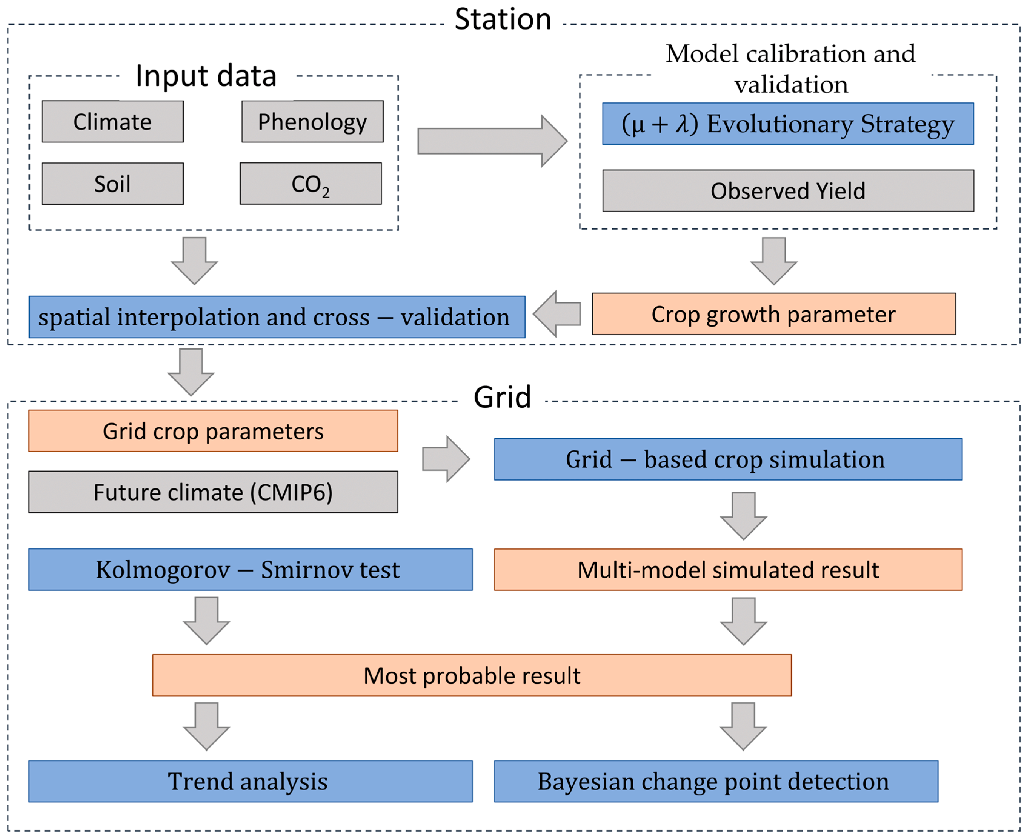
The overall research process is shown in Figure 2.

Figure 2.
Grid crop simulation and analysis flowchart. The gray squares represent the input data, the blue squares represent the method used, and the orange squares represent the processing results.
3. Results
3.1. Spatial–Temporal Variations of Future Cotton Yield in the TRB
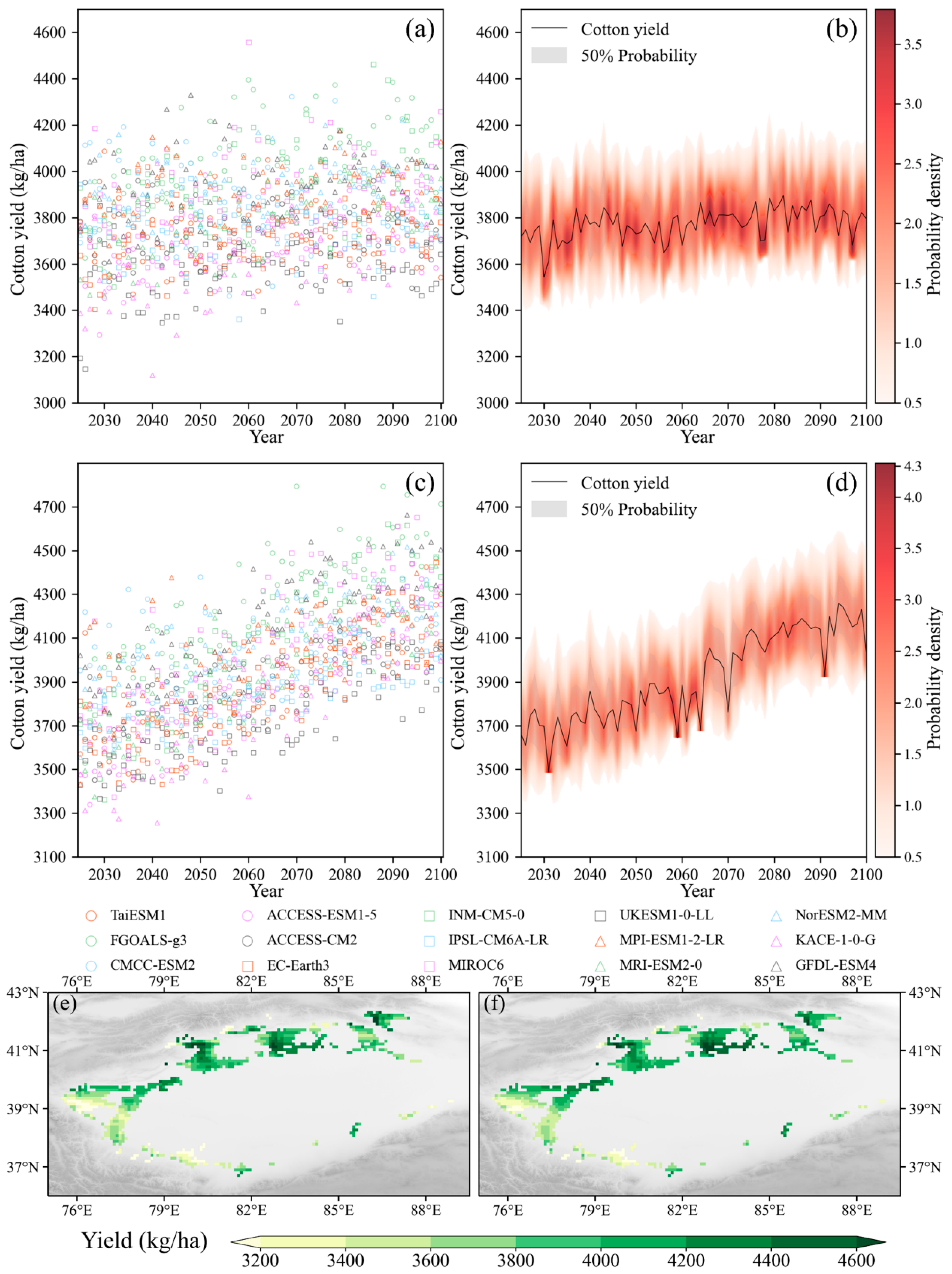
From the results of the multi-model simulations (Figure 3a,c), it can be seen that while most of the GCMs produced results that were concentrated within a narrow range of yields, some models showed significant differences. For example, when using climate data from the FGOALS-g3 model as the input, higher yields were simulated for most years compared to the other GCMs under both climate change scenarios. In order to better identify the trends in the future yield changes and quantify the uncertainty in the yield changes, the study performed goodness-of-fit tests on the multi-model ensemble of cotton yield projections from 2025 to 2100 under two climate change scenarios using the KS test (Figure S1). At a significance level of , the log-logistic distribution was optimal for SSP245, with 74 years of simulated results following the distribution, while the exponentially modified Gaussian distribution was optimal for SSP585, with 73 years of simulated results following it.

Figure 3.
Temporal trends and spatial distributions of cotton yield in the Tarim River Basin from 2025 to 2100 under different climate scenarios. (a) Yield simulation results from 15 sets of GCMs under the SSP245 scenario. (b) The cotton yield trend was calculated based on the simulation results and the optimal distribution under SSP245. The different shades of red represent the probability density, and the line connects the maximum probability density point for each year. The gray shaded area labeled “50% probability” indicates the most likely cotton yield range with a 50% probability. Only the part with a probability density greater than 0.5 is plotted. (c,d) The corresponding results under SSP585. The average values of all the regions reported in this study were calculated by weighing the area of each grid cell. (e,f) The spatial distribution of the average cotton yield under SSP245 and SSP585, respectively.
Based on the fitting results obtained from the best-fit distribution (Figure 3b,d), the probability density of the yield changes captured the concentrated range and overall trend of the simulation results very well. This indicated that the probability density of the best-fit distribution could effectively express the changing information contained in the multi-model ensemble and quantify the uncertainty within the ensemble. Therefore, the study used the yield corresponding to the maximum probability density as the final prediction and analyzed its changing characteristics in the future.
According to the prediction results (Figure 3b,d), the cotton yield showed an increasing trend under both scenarios in the future. Under SSP245, the cotton yield slowly increased at a rate of 13.82 kg/ha/10a (10 years), while under the more severe warming conditions of SSP585, it increased at a rate of 80.68 kg/ha/10a. It is worth noting that there was a significant difference in the interannual variability of the yield between the two climate scenarios. Under SSP245, the coefficient of variation in the yield after detrending was 0.016, whereas under SSP585, it increased to 0.024. This indicated that more severe climate change could intensify the interannual variability of the yield, making it more unstable. Such variations were reflected in SSP585, where sudden drops in the yield in some years were followed by a return to normal fluctuations in the following years. This kind of change can be extremely detrimental to agricultural production and seriously affect the production enthusiasm of farmers [57].
Looking at the cotton yield in the different regions in the future (Figure 3e,f), the spatial distribution pattern under the SSP245 and SSP585 scenarios was quite similar. The southwestern part of the TRB had lower yields, mostly below 3600 kg/ha, while the northern and northwestern plains had higher yields, with the highest cotton yield occurring in the basin’s northern plains, reaching over 4200 kg/ha. Furthermore, under SSP585, the cotton yield in many areas of the basin’s northern plains reached over 4400 kg/ha, whereas there was no significant difference in the average yield in the southwestern part of the basin under either scenario.
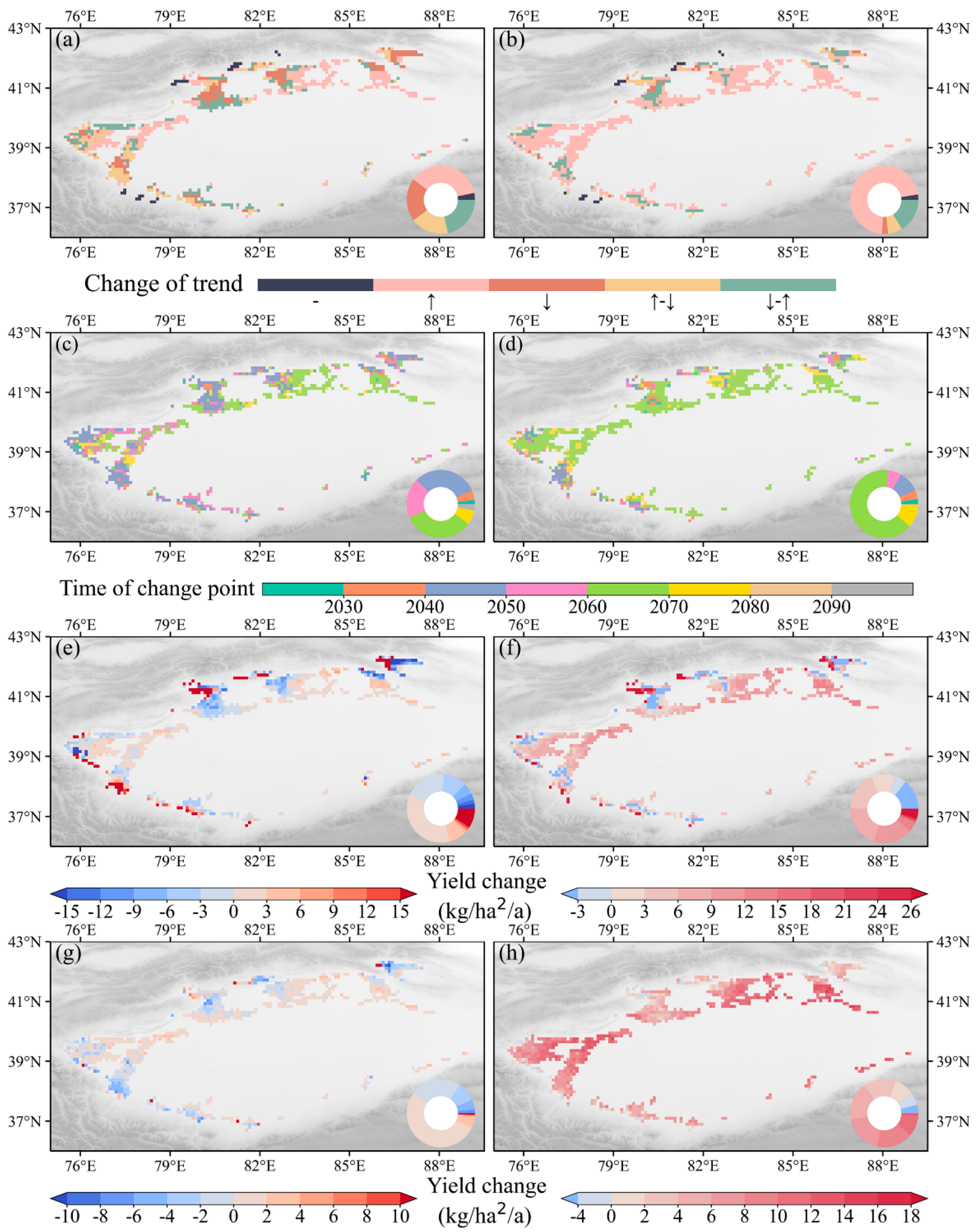
To analyze the trend change of the cotton yield in different regions of the basin further, the study conducted Bayesian change-point detection on each pixel. The detection results (Figure 4) showed that under SSP245, cotton in nearly half of the region exhibited a continuous upward trend, mainly distributed in the northern plains of the basin, with the change-point time concentrated in 2060 to 2070. Two trends—a continuous decline and a decline followed by an increase—mainly occurred in the northwestern TRB, with the change-point time concentrated in 2040 to 2050. However, under SSP585, most of the region was dominated by a continuous upward trend, while the areas that showed a continuous decline under SSP245 also turned into a declining trend followed by an increasing one. Therefore, under SSP585, nearly 75% of the TRB showed a continuous upward trend, and most of the change-point time was during 2060 to 2070.
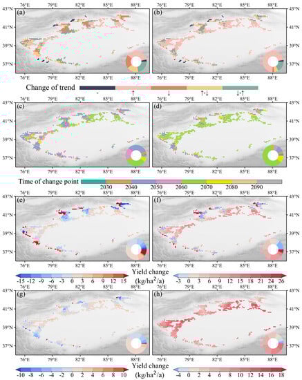
Figure 4.
Variations and trends in the yield changes from 2025 to 2100 under different climate change scenarios in the Tarim River Basin. The results for the SSP245 scenarios are shown in (a,c,e,g), while (b,d,f,h) show the results for the SSP585 scenarios. (a,b) The trend of the yield changes. “−” indicates a simulated yield accumulation of zero for more than three years between 2025 to 2100, so the trend was not analyzed. “↑”, “↓”, “↑−↓”, and “↓−↑” represent “a continuous increase”, “a continuous decrease”, “an increase followed by a decrease”, and “a decrease followed by an increase”, respectively, in the trend before and after the change point. (c,d) The time of the change point. (e,f) The trend before the change point. (g,h) The trend after the change point. The colored ring in the lower right corner of the figure represents the proportion of the different types of pixels.
It is worth noting that the spatial distribution of the areas with a simulated yield accumulation of zero for more than three years was nearly the same in both SSP scenarios and was distributed in the piedmont (foothills) of the TRB. This was mainly because the temperature in the foothills is usually relatively low, making it difficult to meet the heat requirements for crop maturity in colder years. The outcome was an inability to simulate the yield results. Therefore, the study believes that under climate change, the interannual variation in the yield in the TRB’s piedmont regions was too large, meaning that cotton production is not suitable for these areas. A trend analysis was, therefore, not performed.
By further comparing the change trends in cotton yield before and after the change point, the study found that the regions with large changes in both SSP scenarios significantly reduced after the change point, and that most of them were small changes. Even in those piedmont areas that showed a sharp increase in SSP245 before the change point, most had only small increases or decreases after the change point. In terms of the magnitude of changes in different scenarios, the overall change magnitude under SSP245 was smaller than that under SSP585. In addition, in the SSP245 scenario, although the change trend in many locations changed, the overall trend was a small fluctuation between ±3 kg/ha/a, resulting in little variation in the average yield.
3.2. Spatial-Temporal Variations of Future Cotton WPI in the TRB
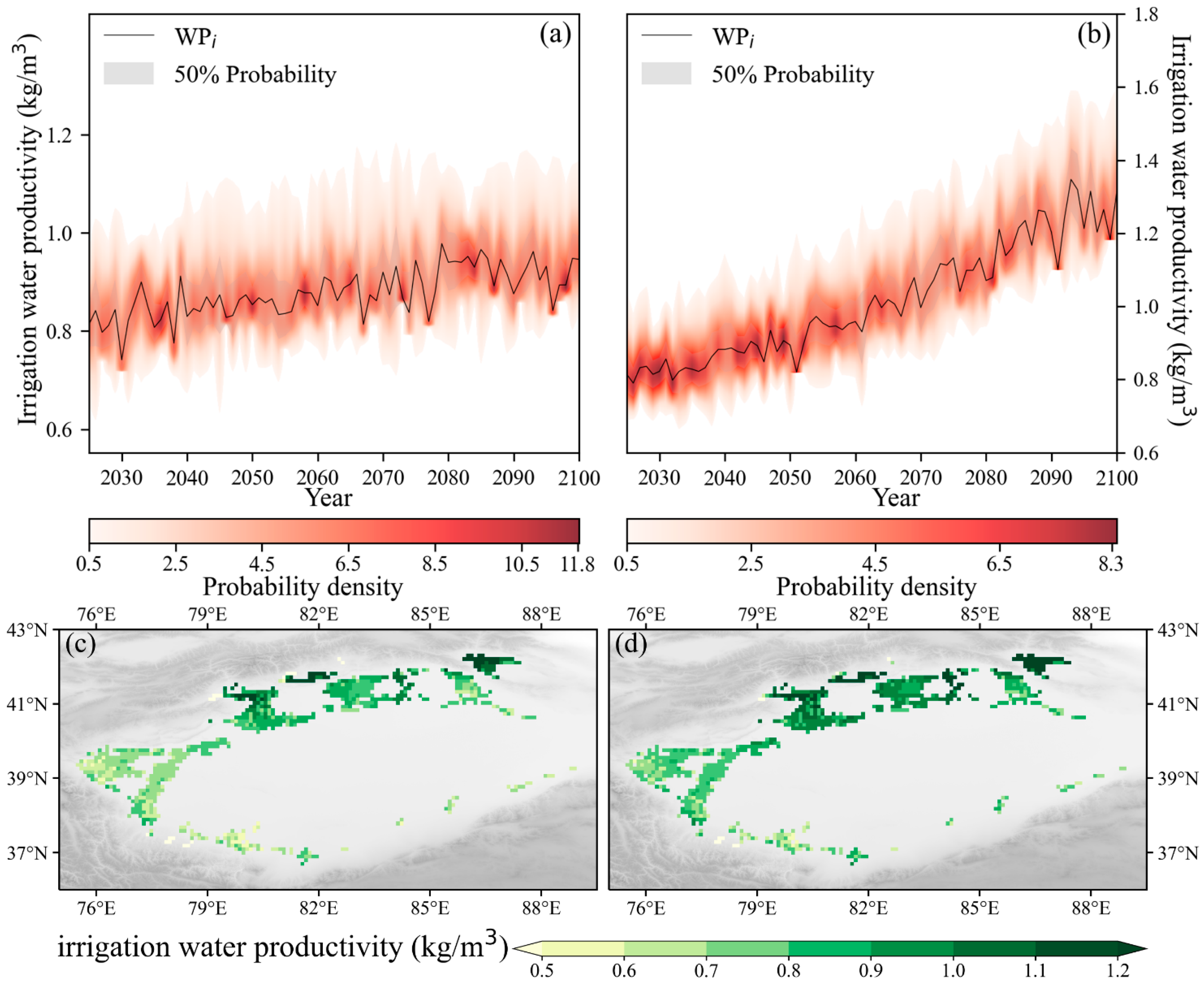
According to the goodness-of-fit test results (Figure S2), the optimal distribution for the future TRB cotton WPI under SSP245 was the Burr Type XII distribution, while under SSP585, it was the exponentially modified Gaussian distribution. The probability density fitted from the optimal distribution (Figure 5a,b) indicated that the future trends of the WPI in different scenarios were similar to those of the yield changes, with both showing an increasing trend. Under SSP245, the WPI increased by 0.015 kg/m3/10a, while under the more severe climate change scenario of SSP585, the increase was even greater, reaching 0.068 kg/m3/10a. However, the WPI showed a greater variability in its future trend changes than its yield, with coefficients of variation of 0.042 and 0.059 under SSP245 and SSP585, respectively.
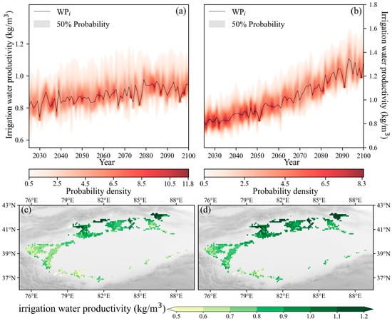
Figure 5.
(a–d) The trend and spatial distribution of the average cotton irrigation water productivity in the Tarim River Basin from 2025 to 2100 under different climate scenarios. (a,b) represent the probability density of the average cotton irrigation water productivity under SSP245 and SSP585, respectively. This was the same as Figure 5c,d, which showed the spatial distribution of the average cotton irrigation water productivity under SSP245 and SSP585, respectively.
The spatial distribution pattern of the WPI was also very similar to that of the yield (Figure 5c,d). In both climate change scenarios, the plains areas with the highest cotton yield in the northern part of the TRB also had a higher WPI, exceeding 0.7 kg/m3 (SSP245) and 0.8 kg/m3 (SSP585). In contrast, the WPI was lower in the southwestern part of the basin. Under SSP585, the average WPI in each region of the study area was generally higher than under SSP245. The highest WPI locations were often located in the piedmont and intermountain basins in the northern part of the TRB. However, the yield in these areas was not necessarily the highest, and some grids even had very low yields. Through an analysis of the relevant climatic factors (Figure S3), the study found that the main reason for this distribution pattern was that the temperatures and reference evapotranspiration were lower in the piedmont areas, while precipitation was significantly higher than in the plains areas, resulting in a lower IR and a higher WPI.
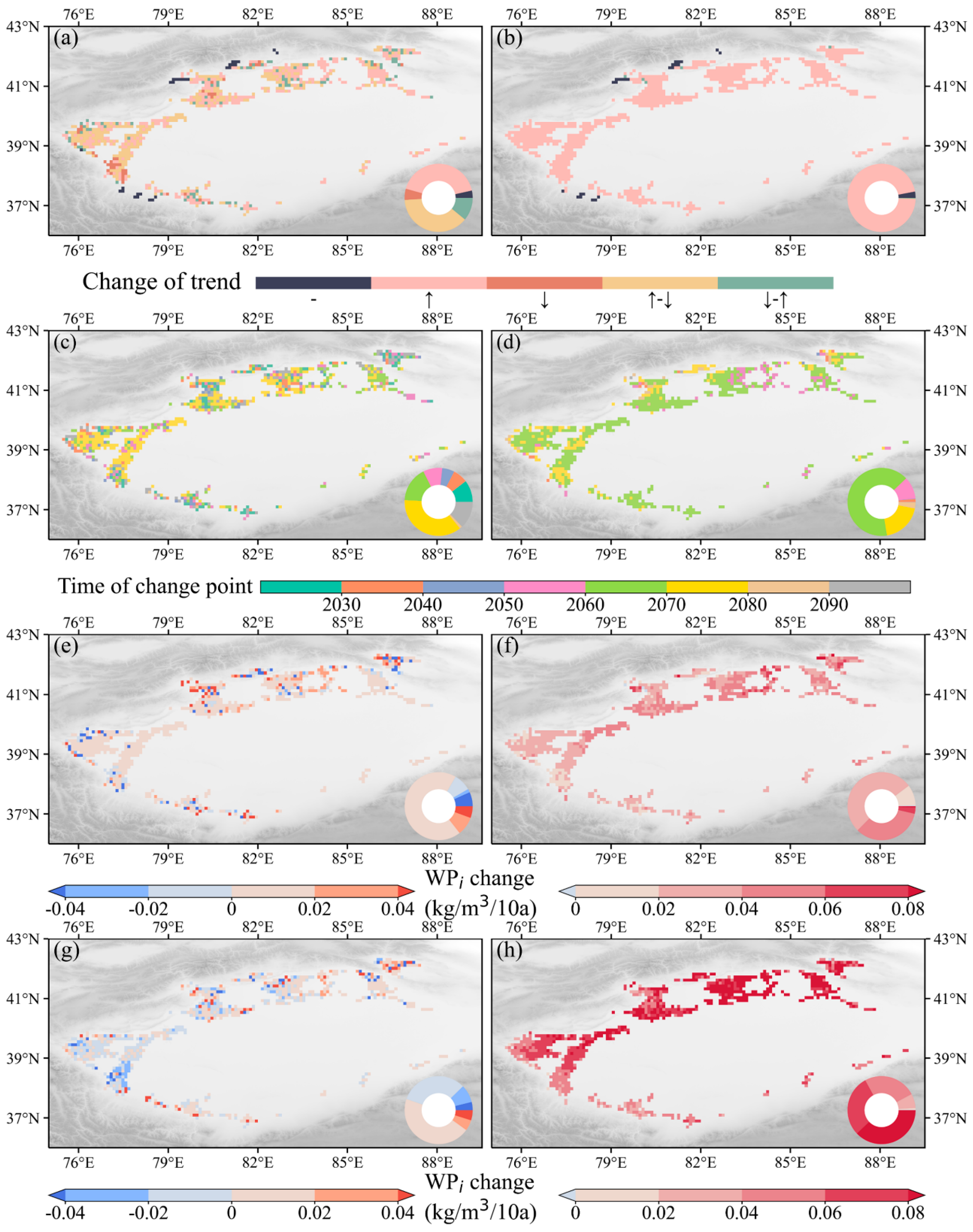
The analysis of the WPI trend changes across the different regions in the future (Figure 6) showed that under SSP585, the WPI in the entire basin had a continuous upward trend. The change point mostly appeared in 2060 to 2070, which was consistent with the yield change point. However, ahead of the change point, the increases were relatively small (0.02–0.06 kg/m3/10a), whereas after the change point they were significantly higher, with most areas reaching more than 0.06 kg/m3/10a. In the plains and intermountain areas in the northern TRB, the increase in the WPI exceeded 0.08 kg/m3/10a. Under SSP245, the trend was mainly a continuous increase and an increase followed by a decrease. The change-point time was relatively dispersed. Although more than half of the locations under SSP245 showed trend changes, the changes before and after the change point were between ± 0.02 kg/m3/10a, which was relatively small. Based on these findings, the overall time series change amplitude of the entire region was not significant.
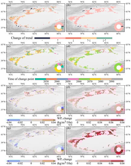
Figure 6.
Change points and trends of the irrigation water productivity in the Tarim River Basin under different climate change scenarios from 2025 to 2100. In (a,b), ‘−’ indicates that the simulated yield and/or irrigation requirements accumulated zero for more than three years during 2025 to 2100. “↑”, “↓”, “↑−↓”, and “↓−↑” represent “a continuous increase”, “a continuous decrease”, “an increase followed by a decrease”, and “a decrease followed by an increase”, respectively, in the trend before and after the change point. (c,d) The time of the change point. (e,f) The trend before the change point. (g,h) The trend after the change point. The colored ring in the lower right corner of the figure represents the proportion of the different types of pixels.
Therefore, considering the spatial distribution and trends for both the WPI and yield, the plains and intermountain areas in the northern TRB exhibited high yields and high WPI, along with a somewhat higher irrigation efficiency compared to the western and southwestern parts of the basin, making them more suitable for cotton production under future climate change.
3.3. FMDI’s Ability to Improve Future Cotton WPI in the TRB
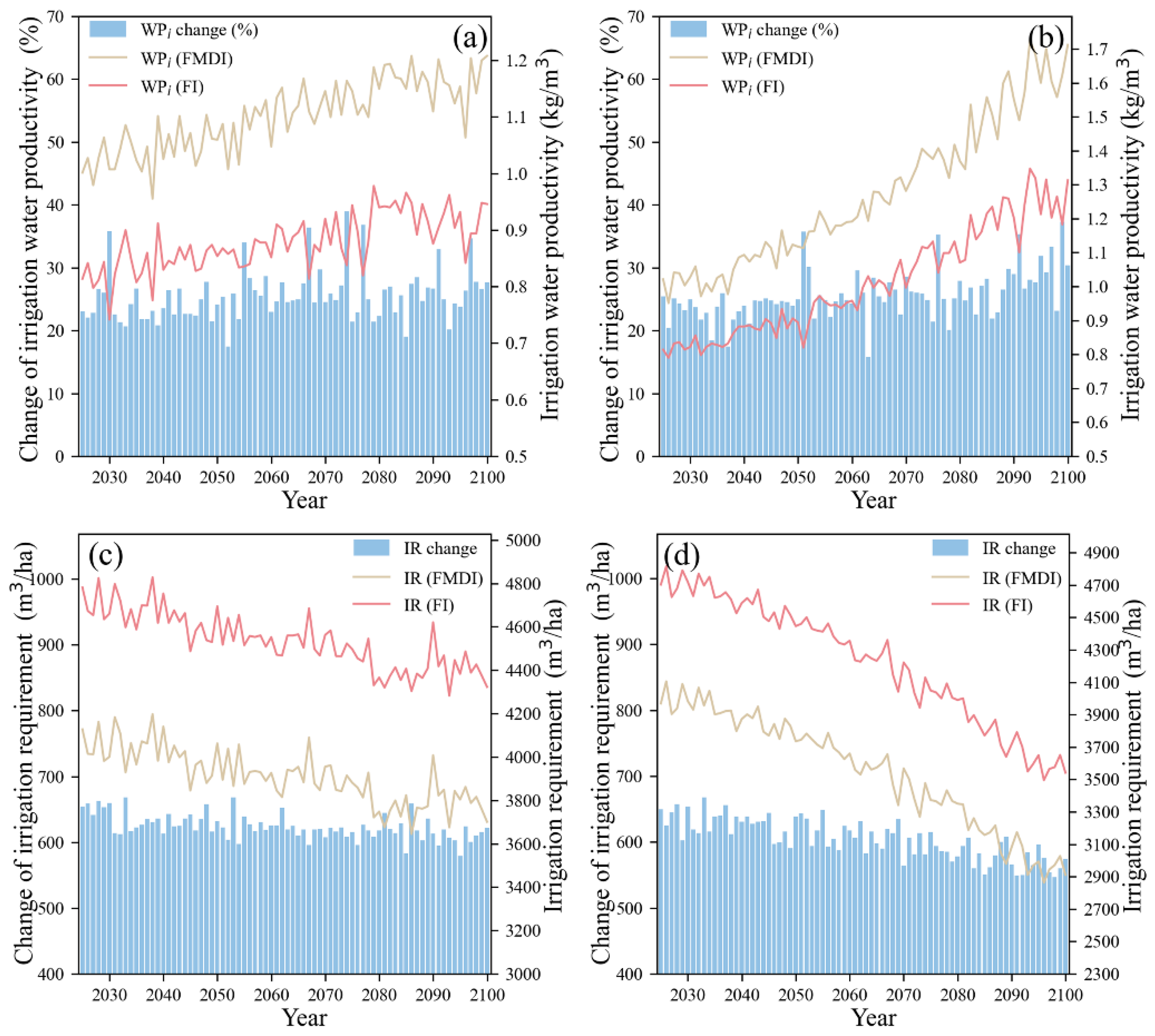
To analyze the water-saving abilities of FMDI in the TRB under climate change, the goodness-of-fit test was performed on the simulation results under FMDI (Figure S4). The change trends of the WPI under two irrigation conditions were then compared. The results (Figure 7a,b) indicated that FMDI showed a good water-saving effect in both of the climate change scenarios, with an average increase of about 25% in the WPI. Moreover, the effect was relatively stable and achieved an increase of over 20% almost every year. Under SSP245, FMDI reduced the interannual variation of the WPI, with the coefficient of variation decreasing from 0.042 to 0.035. However, under SSP585, there was a sharp fluctuation in the WPI after 2080 and the coefficient of variation did not show a significant improvement. From the perspective of the IR changes (Figure 7c,d), the fluctuation trends of the IRs under both irrigation conditions were essentially the same. After using FMDI, the IRs decreased by an average of 624 m3/ha (SSP245) and 605 m3/ha (SSP585). Such reductions in the IRs effectively alleviated the TRB’s agricultural water burden. Interestingly, in this study, the IRs gradually decreased over time, and the FMDI’s reduction in the IRs showed this trend. It is also worth noting that the decrease in the IRs under SSP585 was much greater than that under SSP245.
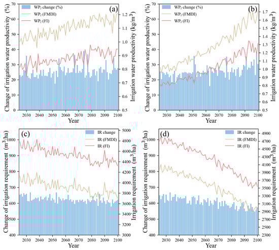
Figure 7.
Changes in the average cotton irrigation water productivity (WPI) and irrigation requirements (IRs) under different irrigation conditions in the Tarim River Basin from 2025 to 2100. (a,b) show the change trend for the average cotton irrigation water productivity under SSP245 and SSP585, respectively, and the bar chart shows the increase in the WPI achieved by adopting film-mulched drip irrigation (FMDI) relative to flood irrigation (FI). (c,d) display the time variations of the average cotton irrigation requirements under SSP245 and SSP585, respectively, while the bar chart shows the reduction in the IRs achieved by using FMDI compared to FI.
From a spatial perspective (Figure 8a,b), the improvement in the WPI using FMDI was generally consistent under both climate change scenarios, with an increase of over 15% in all the locations. However, the increase in the WPI was greater under SSP585 than under SSP245, and there were spatial differences in the degrees of improvement. In the plains areas of the northern and northwestern parts of the TRB, the improvement in the WPI using FMDI was smaller, with increases mainly between 15% and 25%. In contrast, in the intermountain basins and piedmont areas in the northern TRB, the improvement in the WPI was larger, with increases mostly exceeding 35%. However, the reduction in the IRs using FMDI did not show a consistent spatial distribution with the improvement in the WPI (Figure 8c,d), as FMDI could reduce the IRs by almost 550 m3/ha in all the areas.
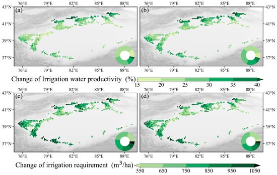
Figure 8.
Improvement capacities of FMDI for the average cotton irrigation water productivity and irrigation requirements in the Tarim River Basin during 2025 to 2100. (a,b) show the improvements in irrigation water productivity using FMDI under SSP245 and SSP585, respectively. (c,d) illustrate the reduced irrigation requirements using FMDI under SSP245 and SSP585, respectively.
The largest reductions in the IRs occurred in the western and southwestern parts of the basin, most of which exceeded 750 m3/ha. The piedmont areas in the southwest showed the greatest reductions (exceeding 950 m3/ha). Meanwhile, the IRs decreased using FMDI in the plains areas of the northern and northwestern parts of the basin where both high yields and a high WPI had been achieved. The results were relatively low, mostly ranging between 550 and 750 m3/ha. Overall, the reduction in the IRs using FMDI was higher under SSP245 than under SSP585, which was opposite to the improvement in the WPI using FMDI.
4. Discussion
4.1. Evaluation of the Simulation Results and Changes in the Cotton Yield and WPI
To assess the errors between the simulated and observed values, the present study evaluated the simulation results by using the RMSE and . The RMSE and for the validation period cotton yield were 131.91 kg/ha and 0.92, respectively. However, AquaCrop’s simulation performance for the cotton yield varied across different studies. Voloudakis [38] simulated the cotton yield in Greece, with the validation results showing an RMSE of 170 kg/ha and a of 0.94, while Tan [23] simulated the cotton yield in Xinjiang, China, obtaining an RMSE of 438 kg/ha and a of 0.82. Compared to these studies, the simulation results in this research were favorable. This suggested that the AquaCrop model, after calibration using the evolutionary strategy, could perform well in the Tarim River Basin.
However, when interpolating the various parameters for the grid-based simulation, there were significant differences in the validation results. The parameters such as HI0 and CCX had good validation results after interpolation, while CGC and HI_Start had poor validation results. This may have been related to the interpolation methods used in the study, as all eight methods used in the research were interpolated based on the spatial distribution and numerical values of the data itself, without introducing any covariates for assistance [58]. Other studies [59,60] have shown that the differences in a range of variables, such as elevation and climatic factors, can significantly affect the performance of the interpolation method. Thus, the accuracy of the interpolation results could be significantly improved by considering the spatial distribution of the covariates. Therefore, in future studies, other interpolation methods that consider covariates or machine-learning methods could be employed to improve the accuracy of the interpolation of the required parameters and further enhance the accuracy of the grid-based simulations [61].
According to the simulation results of this study, cotton yields are projected to increase under both of the future climate change scenarios, with a greater increase occurring under SSP585. This result was consistent with the other research findings [2,62]. The main reason for the projected increase was that in the hypothetical scenarios of the different degrees of climate change in the future, the rise in temperature and CO2 concentrations occur simultaneously. The increase in CO2 concentrations will have a significant water-saving and yield-increasing effect on C3 crops. This effect not only increases the yield, but also reduces crop transpiration and greatly improve the WPI [63]. Additionally, since nearly all the agriculture in the TRB is irrigated, it has a stronger resistance to meteorological drought, so the yield is less affected when drought occurs [38].
Moreover, the increase in the yield variability under SSP585 may be related to the interannual variability of climate factors. Under climate change, climate factors will exhibit a greater interannual variability, and the frequency of extreme weather events will also increase [64], making crops more vulnerable to stress and affecting their normal growth and yield formation [65]. In the warmer SSP585 scenario, the impact is expected to be stronger. Furthermore, the interannual variability of rainfall in the climate factors directly affects the interannual variability of the IRs, which in turn increases the interannual variability of the WPI.
4.2. Influencing Factors of the FMDI’s Water-Saving Capacities
The FMDI’s water-saving effects and its ability to improve the WPI were consistent with the results of the field experiments [15,41]. However, the spatial variability of the FMDI’s ability to improve the WPI was likely related to the crop growth situation. When considering the spatial distribution of the IRs and soil evaporation (Figures S3 and S5), it was observed that the northern and northwestern plains had high IRs and low soil evaporation. On one hand, this was related to the high yield in these regions, which usually means a higher crop transpiration water demand [66]. At this time, soil evaporation accounts for a smaller proportion of water consumption, and the reduction in the IRs caused by FMDI may not be sufficient to cause a significant increase in the WPI. In the TRB’s piedmont areas, the opposite was true. Both the crop transpiration water demand and the IR were lower, indicating that reductions in soil evaporation could easily lead to significant increases in the WPI. In the intermountain basins, due to climatic differences, the ET0 was lower, but when the cotton yield was similar to that in the plains area, the amount of water consumed by crop transpiration was less [67]. Therefore, it would be relatively easy to improve the WPI through FMDI. On the other hand, in the simulation process of the AquaCrop model, when the surface soil was relatively wet, the crop transpiration water demand was mainly extracted from the surface soil [40]. In this case, the simultaneous consumption of crop transpiration and soil evaporation would accelerate the reduction in surface soil water. In the northern and northwestern plains, the water demand for crop transpiration was greater, which further accelerated the consumption rate of surface soil water. However, when the surface soil water decreased to a certain extent, the crop could still obtain transpiration water from the lower soil layers [40], and soil evaporation could enter a decreasing stage. At this time, the amount of soil evaporation is highly dependent on the hydraulic properties of the soil. The simulation results of soil evaporation also reflect this law. In areas with a high yield and reference evapotranspiration, soil evaporation was lower, whereas in areas with low yield, the opposite was true.
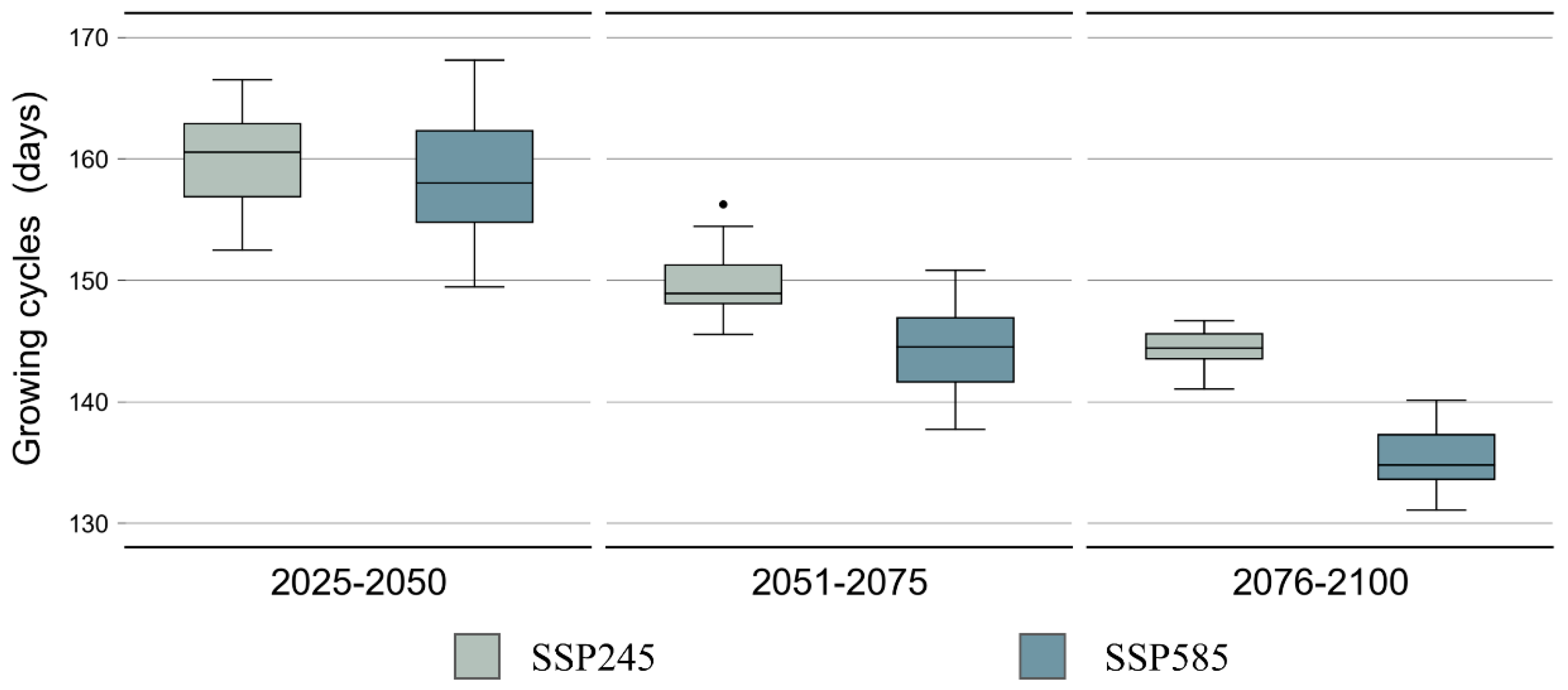
Additionally, the study demonstrated a decreasing trend over time, both in the TRB’s cotton IRs and the FMDI’s ability to reduce the IRs. This decrease was even greater under SSP585 and was mainly related to changes in the crop-growing cycles (Figure 9). Since the study did not consider variety improvement, crop development will likely accelerate with the continuous intensification of climate warming, leading to earlier maturity [68]. Therefore, the reduction in IRs should be consistent with the actual phenomenon. This does not mean that the water-saving ability of FMDI would be affected or that the accuracy of the model simulation is problematic, but that the total amount of soil evaporation and crop transpiration would be reduced due to the shortening of the growth cycle of crops.
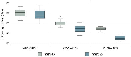
Figure 9.
Changes in the length of cotton-growing cycles under different climate scenarios. The growing cycles are defined as the period from sowing to harvesting. The horizontal line inside the box represents the median; the upper and lower edges of the box represent the 25th and 75th percentiles, respectively; and the whiskers represent a range of 1.5 times the interquartile range (1.5 IQR), with values outside 1.5 IQR not shown. The black dots represent the outliers.
Nevertheless, a warming climate also means the potential for a longer (prolonged) crop-growing period [69]. The related studies have shown that, by adjusting the sowing period of crops, improving the varieties to extend the growing cycle, and fully utilizing the increased heat conditions, the impact of climate change on crops can be alleviated and crop yields can be further improved [70]. However, the IRs will inevitably increase after extending the growing cycle. Therefore, the changes in the WPI when both FMDI and improved varieties are used at the same time still needs further study.
4.3. Shortcomings of AquaCrop and the Study Limitations
Although this study analyzed the water-saving abilities of FMDI under different climate change scenarios and validated its effectiveness as a water-saving measure, there were still some limitations in this work. Firstly, the AquaCrop model only evaluated the impact of FMDI on the IRs in the WPI, while the yield was only considered in terms of its response to climate change. In fact, the use of FMDI greatly improved the soil thermal conditions [19], which was difficult to achieve with organic cover materials such as wheat straw [71]. In regions with poor heat conditions in colder years, the use of FMDI can more easily meet the heat requirements of crops and reduce interannual variations in the yield. The related experimental results showed that these effects further increased the crop yield and improved the WPI [20]. However, the AquaCrop model did not include calculations for the processes involved and could not simulate the increase in the soil temperature and its impact on crops after the use of FMDI. Therefore, the degree of improvement in the WPI shown by FMDI in this study was underestimated, and the actual situation may in fact be even better.
A second limitation concerned the potential spread or conversion of croplands. Although the simulation range integrated all the cropland regions from 1980 to the present, new croplands may appear in other regions or established cropland may convert to a different type of land use. These potential future changes were not simulated here. A third limitation involved the transferability of FMDI. Since FMDI has been shown in this study to achieve water savings by reducing soil evaporation, it is likely to have the same excellent water-saving abilities in irrigated agriculture in other arid regions. However, due to the limitations in the study area, the performance of FMDI in other arid regions still needs further investigation.
5. Conclusions
Based on the site observation data and GCM model output, this study used the AquaCrop model to simulate potential future spatiotemporal changes in cotton yield and cotton WPI under SSP245 and SSP585 scenarios. The study also analyzed the ability of FMDI to improve cotton WPI and reduce IRs. The results showed the following.
(1) Under climate change, the TRB’s cotton yield in different future scenarios show an increasing trend of 13.82 kg/ha/decade (SSP245) and 80.68 kg/ha/decade (SSP585), but there were spatial differences in the extent of these increases. In terms of the spatial distribution, the highest yields occurred in the northern plains and northeastern intermountain basins.
(2) An increasing trend emerged in both the cotton WPI and yield. The rate of increase under SSP245 was 0.015 kg/m3/decade, while under SSP585 it reached 0.068 kg/m3/decade. The spatial differences in the change trend differed slightly from those in the yield. In terms of the spatial distribution, the WPI was higher in the northern and northwestern plains, and in the mountainous basins in the northeast.
(3) With the adoption of FMDI, the TRB’s cotton WPI improved by approx. 25%, and this improvement effect remained stable over time. Spatially, the WPI improvement for all the areas was above 15%, and the reduced IR was mostly above 550 m3/ha. Therefore, FMDI can be an effective water-saving measure in cotton production in the TRB and ensure the stable future development of agriculture in the region.
Supplementary Materials
The following supporting information can be downloaded at: https://www.mdpi.com/article/10.3390/rs15184615/s1, Figure S1: Results of the Kolmogorov-Smirnov test for yield multi-model ensembles under different climate scenarios; Figure S2: Results of the Kolmogorov-Smirnov test for irrigation water productivity multi-model ensembles under different climate scenarios; Figure S3: Annual average temperature, annual precipitation, annual reference evapotranspiration, and annual irrigation requirement under flood irrigation conditions in the Tarim River Basin (2025–2100) for different climate change scenarios; Figure S4: Results of the Kolmogorov-Smirnov test for irrigation water productivity multi-model ensembles under different climate scenarios for film-mulched drip irrigation; Figure S5: Spatial distribution of soil evaporation for different climate scenarios under flood irrigation; Table S1: Fifteen global climate models (GCMs) used in the study; Table S2: Range of crop parameters used in crop model calibration; Table S3: Interpolation methods used in the study and its main parameters; Table S4: Seventeen theoretical distributions used in the study.
Author Contributions
J.Z.: conceptualization, methodology, formal analysis, data curation, visualization, writing—original draft. Y.C.: resources, supervision, funding acquisition, writing—original draft. Z.L.: conceptualization, writing—review and editing. W.D.: writing—review and editing. G.F.: resources. C.W.: data curation, visualization. G.H.: methodology, software, formal analysis. W.W.: conceptualization. All authors have read and agreed to the published version of the manuscript.
Funding
The research was supported by the Tianshan Yingcai Program of the Xinjiang Uygur Autonomous Region (2022TSYCCX0038) and the International Cooperation Program of the Chinese Academy of Sciences (131965KYSB20210045).
Institutional Review Board Statement
Not applicable.
Informed Consent Statement
Not applicable.
Data Availability Statement
The data presented in this study are available upon request from the corresponding authors.
Conflicts of Interest
The authors declare no conflict of interest.
References
- IPCC. Climate Change 2021: The Physical Science Basis. In Contribution of Working Group I to the Sixth Assessment Report of the Intergovernmental Panel on Climate Change; Cambridge University Press: Cambridge, UK, 2021. [Google Scholar]
- Jägermeyr, J.; Müller, C.; Ruane, A.C.; Elliott, J.; Balkovic, J.; Castillo, O.; Faye, B.; Foster, I.; Folberth, C.; Franke, J.A.; et al. Climate impacts on global agriculture emerge earlier in new generation of climate and crop models. Nat. Food 2021, 2, 873–885. [Google Scholar] [CrossRef] [PubMed]
- Hasegawa, T.; Fujimori, S.; Havlík, P.; Valin, H.; Bodirsky, B.L.; Doelman, J.C.; Fellmann, T.; Kyle, P.; Koopman, J.F.L.; Lotze-Campen, H.; et al. Risk of increased food insecurity under stringent global climate change mitigation policy. Nat. Clim. Chang. 2018, 8, 699–703. [Google Scholar] [CrossRef]
- Guan, X.; Ma, J.; Huang, J.; Huang, R.; Zhang, L.; Ma, Z. Impact of oceans on climate change in drylands. Sci. China Earth Sci. 2019, 62, 891–908. [Google Scholar] [CrossRef]
- Lian, X.; Piao, S.; Chen, A.; Huntingford, C.; Fu, B.; Li, L.Z.X.; Huang, J.; Sheffield, J.; Berg, A.M.; Keenan, T.F.; et al. Multifaceted characteristics of dryland aridity changes in a warming world. Nat. Rev. Earth Environ. 2021, 2, 232–250. [Google Scholar] [CrossRef]
- Putnam, A.E.; Broecker, W.S. Human-induced changes in the distribution of rainfall. Sci. Adv. 2017, 3, e1600871. [Google Scholar] [CrossRef]
- Wang, J.; Song, C.; Reager, J.T.; Yao, F.; Famiglietti, J.S.; Sheng, Y.; MacDonald, G.M.; Brun, F.; Schmied, H.M.; Marston, R.A.; et al. Recent global decline in endorheic basin water storages. Nat. Geosci. 2018, 11, 926–932. [Google Scholar] [CrossRef]
- Qin, Y.; Abatzoglou, J.T.; Siebert, S.; Huning, L.S.; AghaKouchak, A.; Mankin, J.S.; Hong, C.; Tong, D.; Davis, S.J.; Mueller, N.D. Agricultural risks from changing snowmelt. Nat. Clim. Chang. 2020, 10, 459–465. [Google Scholar] [CrossRef]
- Yao, J.; Chen, Y.; Guan, X.; Zhao, Y.; Chen, J.; Mao, W. Recent climate and hydrological changes in a mountain–basin system in Xinjiang, China. Earth Sci. Rev. 2022, 226, 103957. [Google Scholar] [CrossRef]
- Koudahe, K.; Sheshukov, A.Y.; Aguilar, J.; Djaman, K. Irrigation-Water Management and Productivity of Cotton: A Review. Sustainability 2021, 13, 10070. [Google Scholar] [CrossRef]
- Fu, J.; Wang, W.; Zaitchik, B.; Nie, W.; Fei, E.X.; Miller, S.M.; Harman, C.J. Critical Role of Irrigation Efficiency for Cropland Expansion in Western China Arid Agroecosystems. Earth’s Future 2022, 10, e2022EF002955. [Google Scholar] [CrossRef]
- Zou, M.; Kang, S. Closing the irrigation water productivity gap to alleviate water shortage in an endorheic basin. Sci. Total Environ. 2022, 853, 158449. [Google Scholar] [CrossRef] [PubMed]
- Li, H.; Mei, X.; Wang, J.; Huang, F.; Hao, W.; Li, B. Drip fertigation significantly increased crop yield, water productivity and nitrogen use efficiency with respect to traditional irrigation and fertilization practices: A meta-analysis in China. Agric. Water Manag. 2021, 244, 106534. [Google Scholar] [CrossRef]
- Ding, Z.; Ali, E.F.; Elmahdy, A.M.; Ragab, K.E.; Seleiman, M.F.; Kheir, A.M.S. Modeling the combined impacts of deficit irrigation, rising temperature and compost application on wheat yield and water productivity. Agric. Water Manag. 2021, 244, 106626. [Google Scholar] [CrossRef]
- Feng, Y.; Hao, W.; Gao, L.; Li, H.; Gong, D.; Cui, N. Comparison of maize water consumption at different scales between mulched and non-mulched croplands. Agric. Water Manag. 2019, 216, 315–324. [Google Scholar] [CrossRef]
- Cheng, M.; Wang, H.; Fan, J.; Zhang, S.; Wang, Y.; Li, Y.; Sun, X.; Yang, L.; Zhang, F. Water productivity and seed cotton yield in response to deficit irrigation: A global meta-analysis. Agric. Water Manag. 2021, 255, 107027. [Google Scholar] [CrossRef]
- Zheng, J.; Fan, J.; Zhang, F.; Zhuang, Q. Evapotranspiration partitioning and water productivity of rainfed maize under contrasting mulching conditions in Northwest China. Agric. Water Manag. 2021, 243, 106473. [Google Scholar] [CrossRef]
- Kader, M.A.; Senge, M.; Mojid, M.A.; Ito, K. Recent advances in mulching materials and methods for modifying soil environment. Soil Tillage Res. 2017, 168, 155–166. [Google Scholar] [CrossRef]
- Mo, F.; Li, X.Y.; Niu, F.J.; Zhang, C.R.; Li, S.K.; Zhang, L.; Xiong, Y.C. Alternating small and large ridges with full film mulching increase linseed (Linum usitatissimum L.) productivity and economic benefit in a rainfed semiarid environment. Field Crops Res. 2018, 219, 120–130. [Google Scholar] [CrossRef]
- Zhou, L.-M.; Li, F.-M.; Jin, S.-L.; Song, Y. How two ridges and the furrow mulched with plastic film affect soil water, soil temperature and yield of maize on the semiarid Loess Plateau of China. Field Crops Res. 2009, 113, 41–47. [Google Scholar] [CrossRef]
- Zhang, M.; Dong, B.; Qiao, Y.; Yang, H.; Wang, Y.; Liu, M. Effects of sub-soil plastic film mulch on soil water and salt content and water utilization by winter wheat under different soil salinities. Field Crops Res. 2018, 225, 130–140. [Google Scholar] [CrossRef]
- Chen, N.; Li, X.; Šimůnek, J.; Zhang, Y.; Shi, H.; Hu, Q.; Xin, M. Evaluating soil salts dynamics under biodegradable film mulching with different disintegration rates in an arid region with shallow and saline groundwater: Experimental and modeling study. Geoderma 2022, 423, 115969. [Google Scholar] [CrossRef]
- Tan, S. Performance of AquaCrop model for cotton growth simulation under film-mulched drip irrigation in southern Xinjiang, China. Agric. Water Manag. 2018, 196, 99–113. [Google Scholar] [CrossRef]
- Ngwira, A.R.; Aune, J.B.; Thierfelder, C. DSSAT modelling of conservation agriculture maize response to climate change in Malawi. Soil Tillage Res. 2014, 143, 85–94. [Google Scholar] [CrossRef]
- Feng, P.; Wang, B.; Macadam, I.; Taschetto, A.S.; Abram, N.J.; Luo, J.-J.; King, A.D.; Chen, Y.; Li, Y.; Liu, D.L.; et al. Increasing dominance of Indian Ocean variability impacts Australian wheat yields. Nat. Food 2022, 3, 862–870. [Google Scholar] [CrossRef] [PubMed]
- Raes, D.; Steduto, P.; Hsiao, T.C.; Fereres, E. AquaCrop—The FAO Crop Model to Simulate Yield Response to Water: II. Main Algorithms and Software Description. Agron. J. 2009, 101, 438–447. [Google Scholar] [CrossRef]
- Liu, B.; Asseng, S.; Müller, C.; Ewert, F.; Elliott, J.; Lobell, D.B.; Martre, P.; Ruane, A.C.; Wallach, D.; Jones, J.W.; et al. Similar estimates of temperature impacts on global wheat yield by three independent methods. Nat. Clim. Chang. 2016, 6, 1130–1136. [Google Scholar] [CrossRef]
- Zhao, C.; Liu, B.; Piao, S.; Wang, X.; Lobell, D.B.; Huang, Y.; Huang, M.; Yao, Y.; Bassu, S.; Ciais, P.; et al. Temperature increase reduces global yields of major crops in four independent estimates. Proc. Natl. Acad. Sci. USA 2017, 114, 9326–9331. [Google Scholar] [CrossRef]
- Zheng, H.; Wei, X.; Tada, R.; Clift, P.D.; Wang, B.; Jourdan, F.; Wang, P.; He, M. Late Oligocene-early Miocene birth of the Taklimakan Desert. Proc. Natl. Acad. Sci. USA 2015, 112, 7662–7667. [Google Scholar] [CrossRef]
- Li, Z.; Liu, T.; Huang, Y.; Peng, J.; Ling, Y. Evaluation of the CMIP6 Precipitation Simulations Over Global Land. Earth’s Future 2022, 10, e2021EF002500. [Google Scholar] [CrossRef]
- Lange, S. Trend-preserving bias adjustment and statistical downscaling with ISIMIP3BASD (v1.0). Geosci. Model Dev. 2019, 12, 3055–3070. [Google Scholar] [CrossRef]
- Allen, R.G.; Pereira, L.S.; Raes, D.; Smith, M. Crop Evapotranspiration—Guidelines for Computing Crop Water Requirements—FAO Irrigation and Drainage Paper 56. Available online: https://www.fao.org/3/X0490E/X0490E00.htm (accessed on 10 September 2020).
- FAO; IIASA; ISRIC; ISSCAS; JRC. Harmonized World Soil Database (Version 1.2). Available online: http://webarchive.iiasa.ac.at/Research/LUC/External-World-soil-database/HTML/ (accessed on 10 September 2020).
- Committee, X.S.Y. Xinjiang Statistical Yearbook. Available online: https://tjj.xinjiang.gov.cn/tjj/zhhvgh/list_nj1.shtml (accessed on 10 September 2020).
- Xu, X.; Liu, J.; Zhang, S.; Li, R.; Yan, C.; Wu, S. Remote sensing data set of multi-period land use monitoring in China(CNLUCC). In Resource and Environmental Science Data Registration and Publication System; Resource and Environment Science and Data Center: Beijing, China, 2018. [Google Scholar] [CrossRef]
- Jiang, T.; Sun, S.; Li, Z.; Li, Q.; Lu, Y.; Li, C.; Wang, Y.; Wu, P. Vulnerability of crop water footprint in rain-fed and irrigation agricultural production system under future climate scenarios. Agric. For. Meteorol. 2022, 326, 109164. [Google Scholar] [CrossRef]
- Iqbal, M.A.; Shen, Y.; Stricevic, R.; Pei, H.; Sun, H.; Amiri, E.; Penas, A.; del Rio, S. Evaluation of the FAO AquaCrop model for winter wheat on the North China Plain under deficit irrigation from field experiment to regional yield simulation. Agric. Water Manag. 2014, 135, 61–72. [Google Scholar] [CrossRef]
- Voloudakis, D. Prediction of climate change impacts on cotton yields in Greece under eight climatic models using the AquaCrop crop simulation model and discriminant function analysis. Agric. Water Manag. 2015, 147, 116–128. [Google Scholar] [CrossRef]
- Kelly, T.D.; Foster, T. AquaCrop-OSPy: Bridging the gap between research and practice in crop-water modeling. Agric. Water Manag. 2021, 254, 106976. [Google Scholar] [CrossRef]
- Dirk, R.; Steduto, P.; Hsiao, T.C.; Fereres, A.E. FAO Crop-Water Productivity Model to Simulate Yield Response to Water. Available online: https://www.fao.org/aquacrop/resources/referencemanuals/en/ (accessed on 10 September 2020).
- Li, S.X.; Wang, Z.H.; Li, S.Q.; Gao, Y.J.; Tian, X.H. Effect of plastic sheet mulch, wheat straw mulch, and maize growth on water loss by evaporation in dryland areas of China. Agric. Water Manag. 2013, 116, 39–49. [Google Scholar] [CrossRef]
- Guo, D.; Olesen, J.E.; Pullens, J.W.M.; Guo, C.; Ma, X. Calibrating AquaCrop model using genetic algorithm with multi-objective functions applying different weight factors. Agron. J. 2021, 113, 1420–1438. [Google Scholar] [CrossRef]
- Zhu, A.X.; Lu, G.N.; Liu, J.; Qin, C.Z.; Zhou, C.H. Spatial prediction based on Third Law of Geography. Ann. GIS 2018, 24, 225–240. [Google Scholar] [CrossRef]
- Zhu, A.; Lv, G.; Zhou, C.; Qin, C. Geographic Similarity: Third Law of Geography? J. Geo-Inf. Sci. 2020, 22, 673–679. [Google Scholar] [CrossRef]
- Choudhury, M.R.; Mellor, V.; Das, S.; Christopher, J.; Apan, A.; Menzies, N.W.; Chapman, S.; Dang, Y.P. Improving estimation of in-season crop water use and health of wheat genotypes on sodic soils using spatial interpolation techniques and multi-component metrics. Agric. Water Manag. 2021, 255, 107007. [Google Scholar] [CrossRef]
- Wu, Y.-H.; Hung, M.-C.; Patton, J. Assessment and visualization of spatial interpolation of soil pH values in farmland. Precis. Agric. 2013, 14, 565–585. [Google Scholar] [CrossRef]
- Rodrigues, G.C.; Pereira, L.S. Assessing economic impacts of deficit irrigation as related to water productivity and water costs. Biosyst. Eng. 2009, 103, 536–551. [Google Scholar] [CrossRef]
- Pereira, L.S.; Cordery, I.; Iacovides, I. Improved indicators of water use performance and productivity for sustainable water conservation and saving. Agric. Water Manag. 2012, 108, 39–51. [Google Scholar] [CrossRef]
- Fernández, J.E.; Alcon, F.; Diaz-Espejo, A.; Hernandez-Santana, V.; Cuevas, M.V. Water use indicators and economic analysis for on-farm irrigation decision: A case study of a super high density olive tree orchard. Agric. Water Manag. 2020, 237, 106074. [Google Scholar] [CrossRef]
- Massey, F.J. The kolmogorov-smirnov test for goodness of fit. J. Am. Stat. Assoc. 1951, 46, 68–78. [Google Scholar] [CrossRef]
- Vlček, O.; Huth, R. Is daily precipitation Gamma-distributed? Atmos. Res. 2009, 93, 759–766. [Google Scholar] [CrossRef]
- Zhang, Q.; Sun, P.; Chen, X.; Jiang, T. Hydrological extremes in the Poyang Lake basin, China: Changing properties, causes and impacts. Hydrol. Process. 2011, 25, 3121–3130. [Google Scholar] [CrossRef]
- Birnbaum, Z.W. Numerical Tabulation of the Distribution of Kolmogorov’s Statistic for Finite Sample Size. J. Am. Stat. Assoc. 1952, 47, 425–441. [Google Scholar] [CrossRef]
- Lilliefors, H.W. On kolmogorov-smirnov test for normality with mean and variance unknown. J. Am. Stat. Assoc. 1967, 62, 399–402. [Google Scholar] [CrossRef]
- Zhao, K.; Wulder, M.A.; Hu, T.; Bright, R.; Wu, Q.; Qin, H.; Li, Y.; Toman, E.; Mallick, B.; Zhang, X.; et al. Detecting change-point, trend, and seasonality in satellite time series data to track abrupt changes and nonlinear dynamics: A Bayesian ensemble algorithm. Remote Sens. Environ. 2019, 232, 111181. [Google Scholar] [CrossRef]
- Erdman, C.; Emerson, J.W. bcp: An R package for performing a Bayesian analysis of change point problems. J. Stat. Softw. 2007, 23, 1–13. [Google Scholar] [CrossRef]
- Ji, X.; Cobourn, K.M. Weather Fluctuations, Expectation Formation, and Short-Run Behavioral Responses to Climate Change. Environ. Resour. Econ. 2020, 78, 77–119. [Google Scholar] [CrossRef]
- Qiao, P.; Lei, M.; Yang, S.; Yang, J.; Guo, G.; Zhou, X. Comparing ordinary kriging and inverse distance weighting for soil as pollution in Beijing. Env. Sci. Pollut. Res. Int. 2018, 25, 15597–15608. [Google Scholar] [CrossRef] [PubMed]
- Meng, Q.; Liu, Z.; Borders, B.E. Assessment of regression kriging for spatial interpolation—Comparisons of seven GIS interpolation methods. Cartogr. Geogr. Inf. Sci. 2013, 40, 28–39. [Google Scholar] [CrossRef]
- Berndt, C.; Haberlandt, U. Spatial interpolation of climate variables in Northern Germany—Influence of temporal resolution and network density. J. Hydrol. Reg. Stud. 2018, 15, 184–202. [Google Scholar] [CrossRef]
- Sekulić, A.; Kilibarda, M.; Heuvelink, G.B.M.; Nikolić, M.; Bajat, B. Random Forest Spatial Interpolation. Remote Sens. 2020, 12, 1687. [Google Scholar] [CrossRef]
- Gamage, D.; Thompson, M.; Sutherland, M.; Hirotsu, N.; Makino, A.; Seneweera, S. New insights into the cellular mechanisms of plant growth at elevated atmospheric carbon dioxide concentrations. Plant Cell Env. 2018, 41, 1233–1246. [Google Scholar] [CrossRef]
- Allen, L.H.; Kimball, B.A.; Bunce, J.A.; Yoshimoto, M.; Harazono, Y.; Baker, J.T.; Boote, K.J.; White, J.W. Fluctuations of CO2 in Free-Air CO2 Enrichment (FACE) depress plant photosynthesis, growth, and yield. Agric. For. Meteorol. 2020, 284, 107899. [Google Scholar] [CrossRef]
- AghaKouchak, A.; Chiang, F.; Huning, L.S.; Love, C.A.; Mallakpour, I.; Mazdiyasni, O.; Moftakhari, H.; Papalexiou, S.M.; Ragno, E.; Sadegh, M. Climate Extremes and Compound Hazards in a Warming World. Annu. Rev. Earth Planet. Sci. 2020, 48, 519–548. [Google Scholar] [CrossRef]
- Hasegawa, T.; Sakurai, G.; Fujimori, S.; Takahashi, K.; Hijioka, Y.; Masui, T. Extreme climate events increase risk of global food insecurity and adaptation needs. Nat. Food 2021, 2, 587–595. [Google Scholar] [CrossRef]
- Bennett, D.R.; Harms, T.E. Crop Yield and Water Requirement Relationships for Major Irrigated Crops in Southern Alberta. Can. Water Resour. J. 2011, 36, 159–170. [Google Scholar] [CrossRef]
- Nistor, M.-M.; Cheval, S.; Gualtieri, A.F.; Dumitrescu, A.; Boţan, V.E.; Berni, A.; Hognogi, G.; Irimuş, I.A.; Porumb-Ghiurco, C.G. Crop evapotranspiration assessment under climate change in the Pannonian basin during 1991–2050. Meteorol. Appl. 2017, 24, 84–91. [Google Scholar] [CrossRef]
- Zabel, F.; Muller, C.; Elliott, J.; Minoli, S.; Jagermeyr, J.; Schneider, J.M.; Franke, J.A.; Moyer, E.; Dury, M.; Francois, L.; et al. Large potential for crop production adaptation depends on available future varieties. Glob. Chang. Biol. 2021, 27, 3870–3882. [Google Scholar] [CrossRef] [PubMed]
- He, L.; Asseng, S.; Zhao, G.; Wu, D.; Yang, X.; Zhuang, W.; Jin, N.; Yu, Q. Impacts of recent climate warming, cultivar changes, and crop management on winter wheat phenology across the Loess Plateau of China. Agric. For. Meteorol. 2015, 200, 135–143. [Google Scholar] [CrossRef]
- Minoli, S.; Jagermeyr, J.; Asseng, S.; Urfels, A.; Muller, C. Global crop yields can be lifted by timely adaptation of growing periods to climate change. Nat. Commun. 2022, 13, 7079. [Google Scholar] [CrossRef] [PubMed]
- Li, S.; Li, Y.; Lin, H.; Feng, H.; Dyck, M. Effects of different mulching technologies on evapotranspiration and summer maize growth. Agric. Water Manag. 2018, 201, 309–318. [Google Scholar] [CrossRef]


Disclaimer/Publisher’s Note: The statements, opinions and data contained in all publications are solely those of the individual author(s) and contributor(s) and not of MDPI and/or the editor(s). MDPI and/or the editor(s) disclaim responsibility for any injury to people or property resulting from any ideas, methods, instructions or products referred to in the content. |
© 2023 by the authors. Licensee MDPI, Basel, Switzerland. This article is an open access article distributed under the terms and conditions of the Creative Commons Attribution (CC BY) license (https://creativecommons.org/licenses/by/4.0/).