Article

Characterizing the Effect of Ocean Surface Currents on Advanced Scatterometer (ASCAT) Winds Using Open Ocean Moored Buoy Data

1
Frontier Science Center for Deep Ocean Multispheres and Earth System (FDOMES) and Physical Oceanography Laboratory, Ocean University of China, Qingdao 266100, China
2
Laoshan Laboratory, Qingdao 266237, China
3
College of Marine Technology, Faculty of Information Science and Engineering, Ocean University of China, Qingdao 266100, China
*
Author to whom correspondence should be addressed.
Remote Sens. 2023, 15(18), 4630; https://doi.org/10.3390/rs15184630
Submission received: 29 July 2023 / Revised: 12 September 2023 / Accepted: 15 September 2023 / Published: 21 September 2023

Abstract

:
The ocean surface current influences the roughness of the sea surface, subsequently affecting the scatterometer’s measurement of wind speed. In this study, the effect of surface currents on ASCAT-retrieved winds is investigated based on in-situ observations of both surface winds and currents from 40 open ocean moored buoys in the tropical and mid-latitude oceans. A total of 28,803 data triplets, consisting of buoy-observed wind vectors, current vectors, and ASCAT Level 2 wind vectors, were collected from the dataset spanning over 10 years. It is found that the bias between scatterometer-retrieved wind speed and buoy-observed wind speed is negatively correlated with the ocean surface current speed. The wind speed bias is approximately 0.96 times the magnitude of the downwind surface current. The root-mean-square error between the ASCAT wind speeds and buoy observations is reduced by about 15% if rectification with ocean surface currents is involved. Therefore, it is essential to incorporate surface current information into wind speed calibration, particularly in regions with strong surface currents.

1. Introduction

Conventionally, long-term and high-precision in-situ sea surface winds are mainly obtained from ships, buoys, and coastal weather stations [1,2]. However, these are single-point observations that struggle to satisfy large-scale and real-time ocean wind monitoring. With the continuous developments in satellite remote sensing technology since the 1970s, satellites have become an important way to monitor global surface winds [3]. The main sensors used to measure surface winds include the altimeter, microwave radiometer, scatterometer, and synthetic aperture radar [4,5,6,7]. As the wind blows over the sea surface, short waves with scales of centimeters are formed, giving rise to sea surface roughness [2]. The sea surface backscattering or sea surface brightness temperature measured via microwave sensors is a manifestation of the sea surface roughness, and then a certain empirical relationship between the sea surface roughness and sea surface wind speed, as well as the corresponding retrieval algorithms, can be derived. Because shortwaves in centimeters are generated by the movement of air relative to the sea surface, the wind observed from a scatterometer represents the wind velocity relative to the ocean surface velocity [8,9], which is distinct from the absolute movement of the atmosphere observed via moored buoys.
However, the in-situ observations of long-term and wide-range ocean surface currents are insufficient, particularly in the open ocean, which brings challenges in accurately assessing the effect of ocean surface currents on satellite-remotely sensed winds. In recent decades, studies regarding the effect of strong currents on satellite-remotely sensed winds have been conducted using tropical moored arrays and coastal buoys. To date, a basic understanding of this effect has been reached: the wind speed inferred from a satellite is generally lower (higher) than that measured via in-situ anemometers when the current is toward (against) the direction of surface winds [10,11,12,13,14]. For example, Dickinson et al. [10] and Kelly et al. [11] compared scatterometer-retrieved winds using the Tropical Atmosphere Ocean (TAO) array, concluding that the zonal wind speed observed via the scatterometer was significantly influenced by background zonal currents. A subsequent study by Kelly et al. [12] also showed that the zonal wind speed differences between TAO buoys and a QuickSCAT scatterometer were highly correlated with the observed zonal currents. The conclusions above are mainly drawn from a tropical moored array where zonal currents are dominant, while the representation of such an effect in extra-tropical regions is not documented, primarily due to insufficient moored buoys involving both wind and current observations.
With respect to the quantification of such an effect, Plagge et al. [13] projected the sea surface current velocity onto the wind direction and obtained a near-one-to-one correlation between the projections and the wind speed differences between satellites and buoys, which means that the difference of ~1.0 m/s in the wind speed principally resulted from the surface current of 1.0 m/s. However, only two buoys off the coast of the Gulf of Maine were used in their analysis, and it is still unclear whether their quantitative description is universal to the open ocean. In this paper, we applied the projection method and extended the analysis to the global open ocean to propose a general quantitative relationship between surface current and wind speed difference. McGregor et al. [14] attempted to correct the satellite-retrieved ocean surface winds and found the inadequacy of using a monthly top 30 m average current product. In this paper, we utilize hourly buoy-observed ocean currents at the very near surface to correct scatterometer winds. By removing the wind bias caused by background currents, the root-mean-square error (RMSE) between the in-situ observed wind speed and advanced scatterometer (ASCAT)-retrieved wind speed is expected to be significantly reduced. Additionally, a reprocessed surface current product is used for comparison in the correction process.
This paper is organized as follows. The data preprocessing and methods are introduced in Section 2. The detailed results, including the data comparison between buoys and ASCAT, the wind speed difference and its relationship with the surface current, and the correction of the ASCAT-retrieved winds, are described in Section 3. Discussions are presented in Section 4, followed by conclusion in Section 5.

2. Data and Methods

The remotely sensed wind speed and direction are obtained from two ASCAT product sets [15,16]. ASCAT is one of the instruments carried onboard the Metop polar satellites launched by the European Space Agency. Retrievals from the C-band ASCAT scatterometers onboard Metop-A and Metop-B show comparable statistics when compared to reanalysis winds [17]. The Level 2 (L2) and Level 3 (L3) ocean surface wind products derived from ASCAT are two types of commonly used satellite wind products. The L3 wind product relies on the L2 scatterometer wind vectors, which are re-gridded to a regular Lat-Lon grid with fixed spacing. To assess whether the accuracy of the L3 ASCAT wind speed diminishes or not after this meshing and averaging process, and to what extent the contribution of the surface current is inherited in this wind product, a comparison is made between data from the ASCAT L2 and L3 products. The Metop-B ASCAT L2 along-track data and the Metop-A ASCAT L3 daily instantaneous gridded data are collected over a 10 yr and 15 yr time period, respectively. The two scatterometer datasets are calibrated to approximate the wind at 10 m above the ocean surface in a neutrally stratified atmosphere with a spatial resolution of 25 km. Additionally, to fulfill the requirement for the simultaneous observation of the sea surface current and wind, a total of 40 mooring buoys were chosen, including buoys from Tropical Atmosphere Ocean/Triangle Trans-Ocean Buoy Network (TAO/TRIRTON), Prediction and Research Moored Array in the Tropical Atlantic (PIRATA), Research Moored Array for African–Asian–Australian Monsoon Analysis and Prediction (RAMA), and several other buoys at the mid-latitudes (Figure 1). These buoys provide high-temporal-resolution observations, with data recorded at 1 h intervals.
For the L2 along-track product, data pairs that contain ASCAT wind and buoy wind are collected when the scatterometer cell center is within 25 km of a moored buoy and the time lag is less than 30 min [10]. Then, all scatterometer data that meet the above criteria are averaged, generating a unique data pair of hourly winds [12]. For L3 daily instantaneous gridded data, the acquisition time of measurements is provided for each grid point. The scatterometer wind vectors are interpolated to the location of the moored buoy by means of nearest interpolation if the time lag is less than 30 min. A total of 28,803 (40,426) data triplets, consisting of buoy-observed wind vectors, current vectors, and ASCAT L2 (L3) wind vectors, were collected from the dataset spanning over 15 years. The numbers of triplets at each buoy station, during the period from 1 January 2007 to 31 December 2021, are shown in Figure 2.
To allow a comparison with the scatterometer-retrieved winds, the buoy-observed winds are adjusted to a 10 m neutral stability wind using the Coupled Ocean–Atmosphere Response Experiment (COARE) 3.0 bulk flux algorithm [18]. Ancillary buoy measurements, including the air temperature, sea surface temperature, and relative humidity were utilized for this adjustment. The surface velocity was determined via selecting the topmost current velocity measured by the buoy, while ensuring a sufficient data-recording duration. Table 1 presents the relevant information regarding the ocean current measurement sensors utilized by each buoy, along with the corresponding measured depths. The velocity measurements were selected at a minimum depth of 5 m and a maximum depth of 20 m. The hourly buoy-observed currents represent the actual oceanic currents, encompassing geostrophic currents and Ekman currents, as well as ageostrophic factors such as tidal currents. Furthermore, a collection of 3-hourly reprocessed current products with a spatial resolution of 1/4°, obtained from the Copernicus Marine Environment Monitoring Service (CMEMS), was utilized for comparison and ASCAT wind speed correction [19]. The surface ocean current velocities for this product are obtained as the sum of the surface geostrophic current derived from altimetry and the Ekman component, derived by applying an empirical Ekman model to ERA5 wind stress. There is no global bias in the currents, but the zonal velocity is found to be more accurate than the meridional velocity.
The 15-year averaged surface current field from 2007 to 2021 is depicted based on CMEMS data. Moored buoys are spreading in the regions characterized by strong surface currents, including the equatorial current system, wind-driven, and western boundary currents. Additionally, the sea area with a relatively weaker current is also deployed with moored buoys such as Station Papa (Figure 3a). We conducted an analysis of the probability density distribution (PDF) of the current speed and current direction, and the angle between the current direction and the wind direction, based on buoy observations. For this analysis, we employed 28,803 data triplets that included buoy-observed wind vectors, current vectors, and L2 ASCAT-derived wind vectors. These moored buoys provide a wide range of surface current speed observations from near zero to 1.0 m/s, with an average of about 0.23 m/s (Figure 3b). The PDF of current direction exhibits two peaks, at approximately 74° and 268°, respectively, with the peak near 268° being more pronounced (Figure 3c). It should be noted that the surface current direction is represented in the nautical coordinate system, where zero signifies the flow toward true north, with direction proceeding in a clockwise rotation. These observations indicate that the current directions are primarily oriented east–west, with the current from east to west predominant. Further examination of the angle between current direction and wind direction shows that although the surface current directions are mostly in alignment with the surface winds, the angle between them is widely distributed between 0 and 180°. It provides a good dataset for the subsequent analysis of the influence of ocean currents on scatterometer-retrieved winds.
Because a satellite scatterometer measures winds relative to the moving ocean surface, not to a stationary point, the ASCAT winds should be lower than those measured using anemometers when the current is in the same direction as the wind. Conversely, the ASCAT winds should be higher when the current opposes the wind. On one hand, the current effect on the scatterometer wind vector is revealed via analyzing the relationship between the zonal and meridional components of ASCAT wind bias and ocean surface current [10]. On the other hand, the current velocity is projected onto the anemometer’s wind heading direction ( θ w ) and is defined as
u p = u c cos θ c θ w
where u c is the magnitude of the surface current and θ c is the direction of the current in oceanographic convention [13]. Then, the current effect on the scatterometer wind speed is revealed via analyzing the relationship between the ASCAT wind speed bias and the projected current speed u p . It should be noted that the wind biases mentioned in this article were computed via subtracting the anemometer wind from the ASCAT wind. Following the approach described by Plagge et al. [13], we performed a linear least-squares regression analysis to establish the relationship between wind bias and u p . Subsequently, we applied the derived regression equation to correct the scatterometer winds. The correlation coefficient (R) is employed to characterize the relationship between the wind speed bias and the current speed, and the root-mean-square error is used to quantify the discrepancy between the satellite-retrieved winds and buoy-observed winds.

3. Results

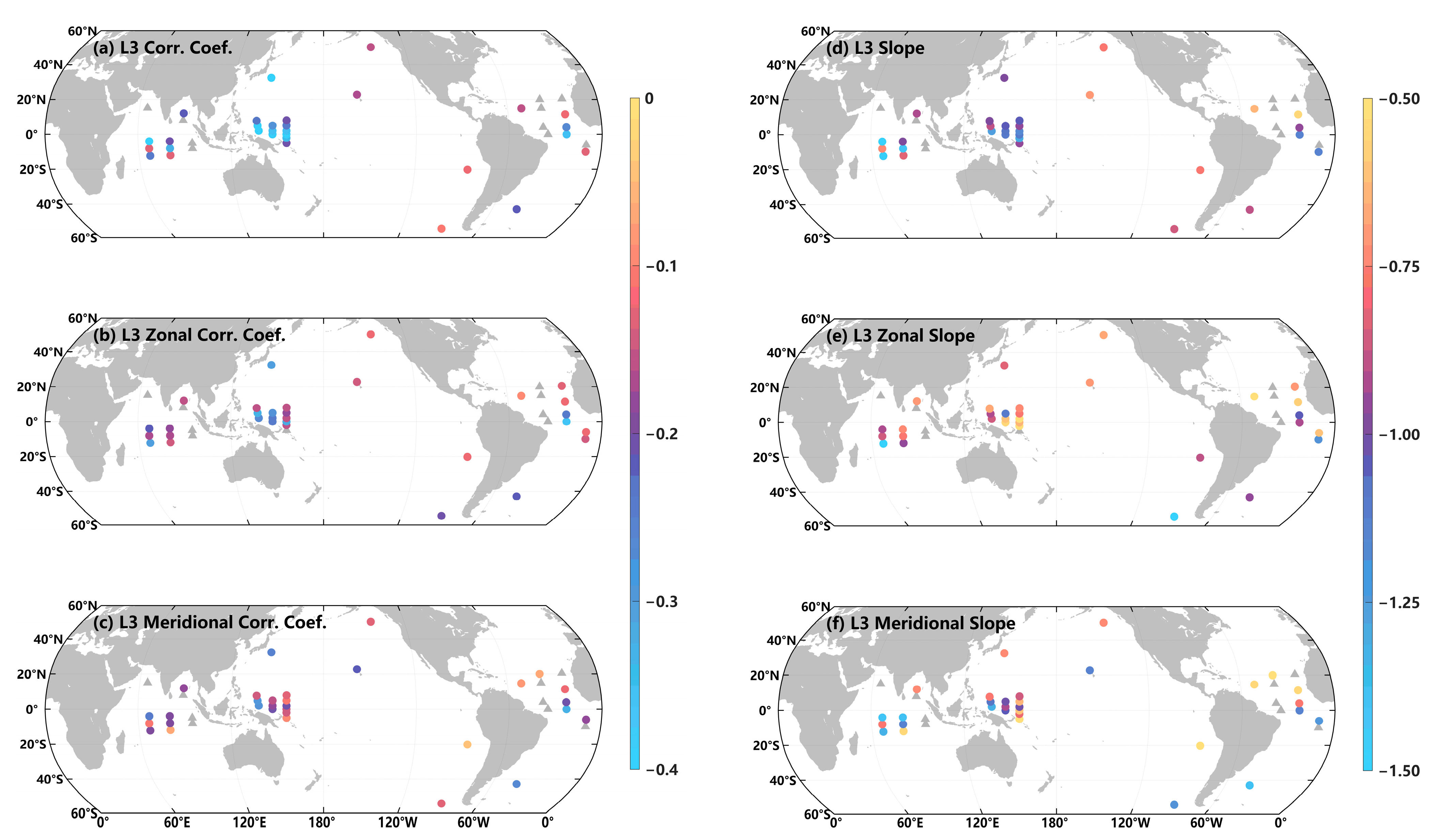
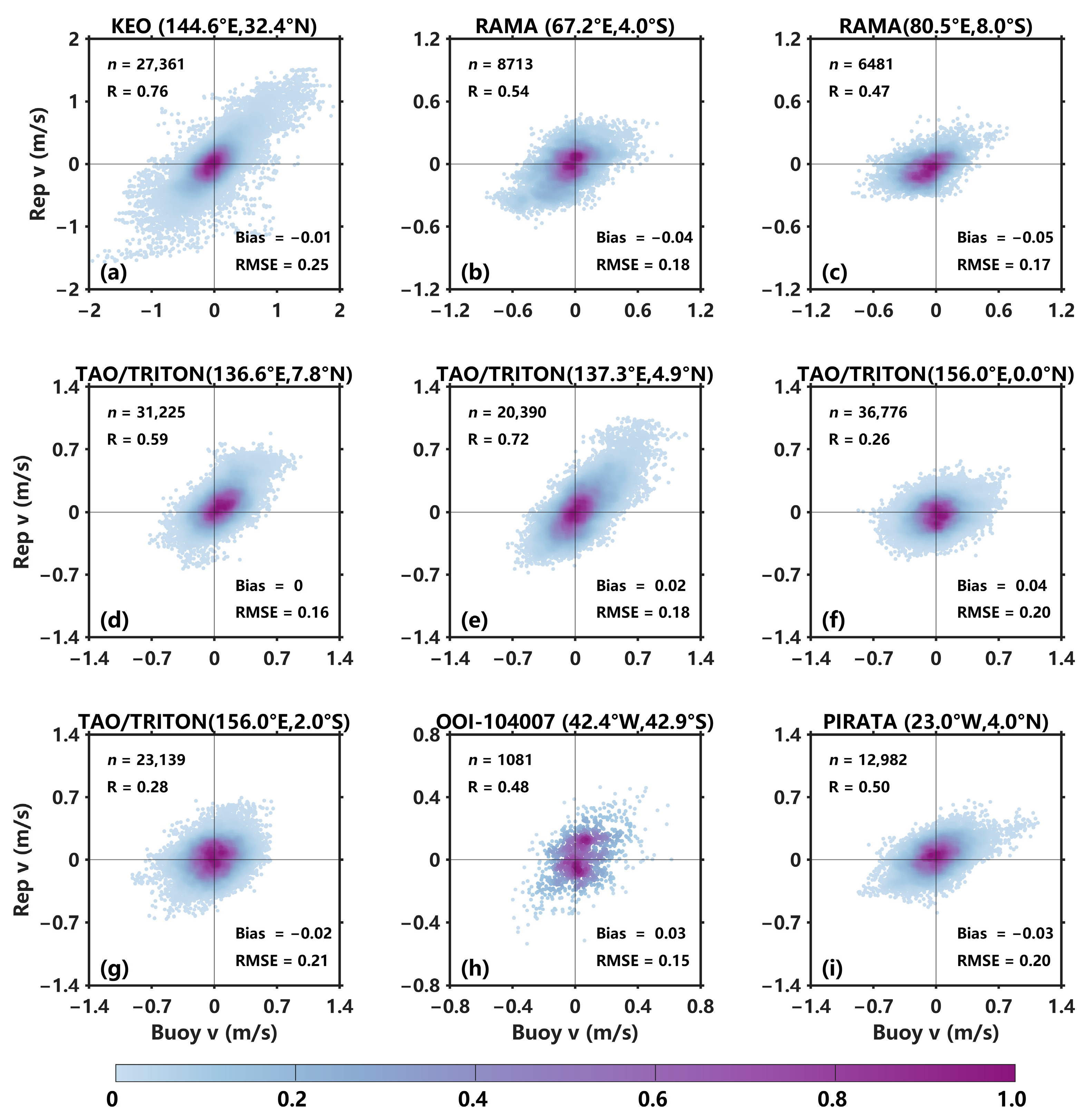
3.1. Effect of Surface Current on Satellite Wind

The buoy winds and scatterometer winds show a good consistency with each other, and the mean biases of both the ASCAT L2 and L3 winds are less than 0.3 m/s (Figure 4). The RMSE of the ASCAT scalar wind speed is about 1.0 m/s. In addition, for either the zonal or meridional components of wind vectors, it is about 1.3 m/s, which is larger due to the scatterometer’s wind direction bias [20]. The ASCAT L3 product underwent an interpolation to a regular Lat–Lon grid firstly, and then an interpolation to the buoy stations. Due to the two interpolations, the wind bias and RMSE for the L3 product are slightly larger compared to those for the ASCAT L2 product.
The equatorial current system, combined with wind-driven and western boundary currents, provides the conditions for intense air–sea interactions and a strong near-surface velocity [21,22]. With moored buoys extensively distributed across these areas, the influence of ocean currents on ASCAT L2 scalar winds is assessed via conducting a linear least-squares regression analysis to determine the relationship between wind speed bias and the projected ocean current u p . The projected current speed approximately satisfies the normal distribution both globally and for tropical ocean basins (Figure 5(a1–d1)). The global average ASCAT L2 wind speed bias is about −0.96 times the magnitude of the projected current speed u p , i.e., the ASCAT L2 winds are lower than the buoy winds when currents are in the same direction as the wind and are stronger when ocean currents oppose the wind. Regional analysis, using buoy data from the RAMA array in the Indian Ocean, the TAO/TRITON array in the tropical western Pacific, and the PIRATA array in the tropical Atlantic Ocean, reveals a consistent negative correlation between ASCAT L2 wind speed bias and u p . The correlation coefficients obtained for these regions are −0.20, −0.31, and −0.21, respectively (Figure 5(b1–d1)).
The ability for wind direction measurements in a satellite scatterometer enables the analysis of the effect of ocean surface currents on ASCAT wind speeds in both zonal and meridional directions. Applying the same analysis methodology employed for the scalar wind speed, the relationship between zonal/meridional wind speed bias and surface velocity is elucidated. Globally, the ASCAT L2 wind biases are −0.78 and −0.81 times the magnitude of the zonal and meridional current velocity, respectively (Figure 5(a2,a3)). The regression slopes for both the zonal and meridional components exhibit significant fluctuations near unity, suggesting that the ambiguity in the ASCAT wind direction contributes to larger errors in two wind speed components. Consequently, the observed deviation in ASCAT wind speed components cannot be solely attributed to ocean currents.
The same analysis is performed with the L3 daily instantaneous gridded data. The ASCAT L3 product is derived from the upstream L2 wind product via interpolating the wind vector cell measurements to a regular Lat–Lon grid. The measurements from the ascending and descending passes are gridded into separate datasets, both of which are used to obtain the triplet containing the satellite wind, buoy wind, and surface current. The ASCAT L3 wind speed bias also exhibits a negative correlation with the projected current speed u p , and the current velocity of 1.0 m/s corresponds to an error of 0.96 m/s in the scalar wind speed (Figure 6(a1)).
The above statistical analyses give us an intuitive impression of the relationship between the scatterometer wind bias and the ocean surface velocity. However, it is interesting to check whether the relationship is consistent in different sea areas. Subsequently, we conduct a detailed analysis of the effect of ocean currents on ASCAT winds at each mooring station. In our analysis of the ASCAT L2 data, we see that 34 out of the 40 buoys exhibit a negative correlation between wind speed bias and the projected surface current speed, with correlation coefficients mainly ranging from −0.3 to −0.1 (Figure 7a). The result suggests that the current projection approach employed by Plagge et al. [13], based on two coastal buoy datasets, can also be applied to the open ocean. The slope of the linear regression equation is close to −1.0 at these stations (Figure 7d); that is to say, in strong ocean currents such as the equatorial countercurrent and western boundary currents [23], the ocean surface velocity of 2.0 m/s will cause an error of the same magnitude in the satellite scatterometer wind speed. The relationships between the zonal and meridional components of the ASCAT L2 wind speed bias and the ocean surface current have also been investigated. The correlation coefficients and slopes obtained are consistent with the analysis of scalar wind speed bias (Figure 7b,c,e,f). Additionally, the zonal component shows a stronger negative correlation than the meridional component.
The correlation between the scatterometer wind residuals and surface current speeds is influenced by the air–sea condition, sea state, and wind speed. In addition, the variation in correlation coefficients is attributed more to a combination of marine environments and statistical effects than to an actual increase or decrease in surface current. Plagge et al. [13] showed that the best correlation is obtained in conditions with a near-neutral atmospheric stability and moderate wind speeds. In general, ocean surface winds and sea states are moderate near the equator and more turbulent in mid-latitude oceans. The variations in marine environments and the unequal distribution of data points may contribute to differences in the correlation coefficients at various sampling locations.
The linear correlation coefficients and slopes are quite similar to Figure 7 in the analysis of the ASCAT L3 wind product (Figure 8), which indicates that the L3 daily instantaneous gridded scatterometer wind product inherits the influence of the ocean surface current existing in the along-track measurements. In summary, a negative correlation is observed between the ASCAT wind speed bias and ocean surface velocity, regardless of the use of different products within the same sea area or of the same product across different sea areas (including tropical and mid-latitude oceans). The correspondence is consistent with the physical understanding that the relative motion of wind and current influences the roughness of the sea surface, resulting in the satellite scatterometer-retrieved wind speed being relative to the moving of the ocean surface. A simple linear relationship between the wind bias and surface current can then be used to correct the ASCAT wind to the absolute movement of the atmosphere.

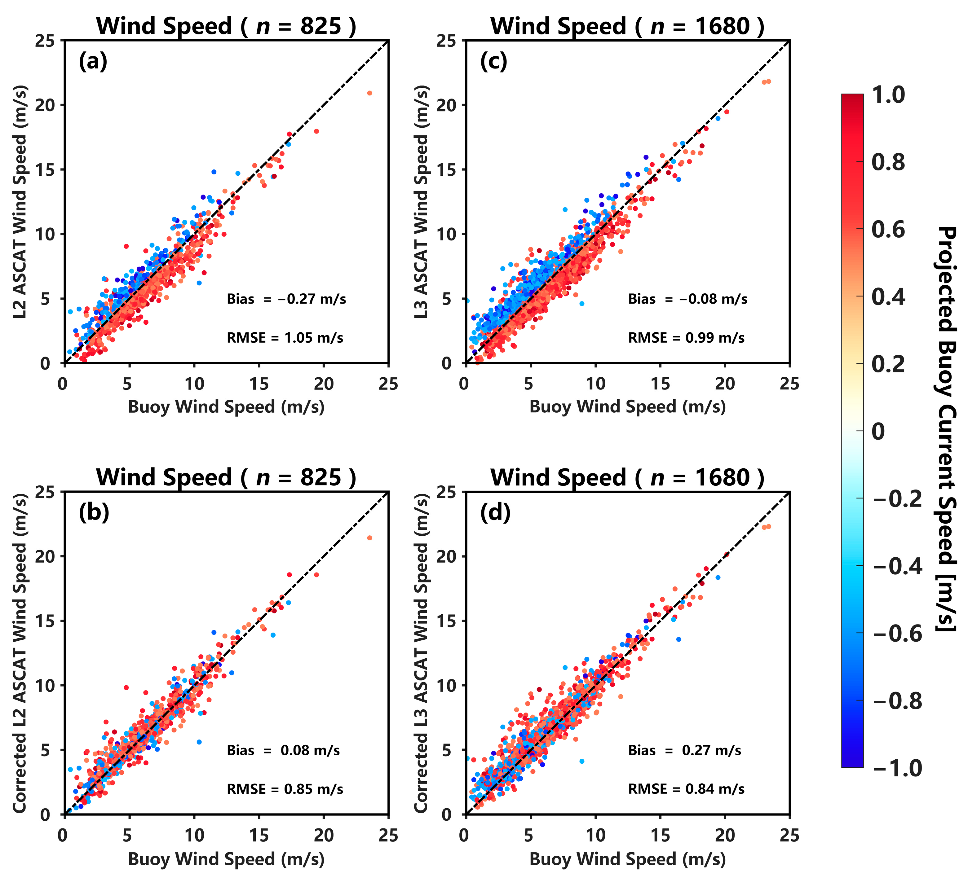
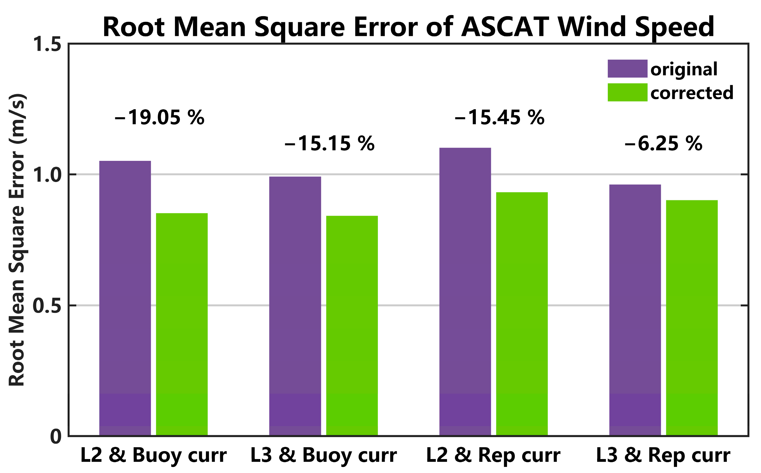
3.2. Correction of Scatterometer-Derived Ocean Surface Wind Speed

As mentioned above, the ocean surface winds derived from a scatterometer are the winds relative to the moving of the ocean surface. Thus, ASCAT winds should be weaker than buoy winds when currents are in the same direction as the wind and vice versa. We have obtained the approximate linear correspondence between the ASCAT wind speed bias and the projected current speed u p as follows:
w i n d   s p e e d   b i a s = k u p
In this section, k u p , where k equals −0.96, was subtracted from the ASCAT scalar wind speed for correction. We assume that the magnitude of the scatterometer wind bias is approximately equal to the surface current speed. To make this assumption valid, the anemometer’s wind needs to be in the same direction as the scatterometer wind. Moreover, only when the surface current speed is strong enough can its effect be revealed. Thus, only the triplets where the anemometer and scatterometer wind directions differed by no more than 30°, and where the current projection was no less than 0.5 m/s, are applied to evaluate the behavior of wind speed correction. These constraint conditions provide a total of 825 triplet matches (scatterometer wind speed, buoy wind speed, and u p ) for the ASCAT L2 data and 1680 matches for the ASCAT L3 data.
The mean bias and RMSE of the wind speed between the ASCAT L2 and buoy observations are −0.27 m/s and 1.05 m/s, respectively. For the ASCAT L3 wind product, they are −0.08 m/s and 0.99 m/s (Figure 9a,c), respectively. The RMSEs of the two sets of satellite scatterometer wind products are both less than 1.5 m/s, which is considered to be acceptable in commercial use, but the distribution of the wind speed bias is closely related to the projected current speed u p . When u p is positive, i.e., the surface wind and ocean current are in the same direction, the ASCAT wind speed is lower than that measured via buoy. On the contrary, the ASCAT wind speed is higher than the buoy measurement when u p is negative. In Figure 9a,c, the positive and negative u p are typically distributed on opposite sides of the boundary where the ASCAT wind speed is equal to the buoy wind speed. However, the distinct characteristic of this distribution is no longer apparent when comparing the corrected ASCAT winds with the buoy winds. Meanwhile, the RMSEs of the ASCAT L2 and L3 wind speeds are reduced to 0.85 m/s and 0.84 m/s (Figure 9b,d), respectively.
Considering that the surface currents measured via mooring buoys are sporadic, it is difficult to correct the satellite scatterometer winds based solely on buoy-observed currents. An attempt was made to utilize a set of reprocessed ocean surface current data obtained from CMEMS as a substitute. This dataset was derived through combining the geostrophic current and the Ekman current at the sea surface (0 m). After comparison with buoy-observed currents in regions with a relatively high surface velocity, the mean bias of the reprocessed current was found to be nearly zero (Figure 10 and Figure 11). In addition, the zonal velocities show a greater consistency with observations compared to the meridional components. The close correlation between the ASCAT wind speed bias and u p can also be broken after the correction using the reprocessed surface current, and the RMSE of the corrected ASCAT wind speed is significantly reduced (Figure 12). After correction using the buoy current and reprocessed current, the RMSE of the L2 ASCAT wind speed decreased by 19.05% and 15.45%, respectively (Figure 13). Ageostrophic signals, such as tidal currents, are excluded from this reprocessed current product. We know that tidal currents in the open ocean exhibit relative weakness compared to those in coastal areas [24]. Furthermore, we set a high current speed threshold of 0.5 m/s for screening, which further mitigated the influence of tidal currents on the assessment of correcting the scatterometer-retrieved wind speed with ocean current data. The linear correlation between ASCAT wind residuals and surface current speed remains valid both in the open ocean and in coastal areas. However, employing the current product that excludes tidal currents for wind correction in coastal areas is not recommended.

4. Discussions

Due to insufficient moored buoys involving both wind and current observations in the extra-tropical regions, the previous works mainly focus on the tropical ocean and coastal areas. Utilizing valuable data obtained from four mid-latitude moored buoys, our study validates that the linear correlation between the scatterometer-retrieved wind bias and the ocean surface current speed is also present at mid-latitudes, which expands the application range of previous studies. McGregor et al. [14] showed that applying the monthly OSCAR current product (top 30 m average) for correction did not reduce the overall bias between the mooring and satellite surface winds. It suggested that the estimation of currents at the very near surface may yield a more significant correction effect. In this study, we used hourly current data measured via moored buoys at the very near surface to correct the wind speed derived from ASCAT. The mean bias and RMSE between the ASCAT-derived and buoy-observed wind speeds are both reduced significantly in strong ocean current conditions.
A satellite scatterometer measures the stress-equivalent wind, which is relative to the moving ocean surface, but the absolute winds measured by the buoy relative to the stationary point are often used to calibrate and verify the scatterometer winds. Our comparisons and analyses suggest that caution will be needed if the buoy is located at a region with strong ocean surface currents (≥0.5 m/s). The current velocity may introduce an error of approximately 10–20% to the validation of wind speed. For regions with strong surface currents, simultaneous observations of surface winds and currents are urgently needed. In the presence of sea surface current data, it is essential to consider the current velocity during the calibration of scatterometer-retrieved ocean surface winds.

5. Conclusions

Based on ASCAT ocean surface winds, as well as simultaneous wind and surface current observations from 40 buoys in the tropical and mid-latitude ocean, this study characterizes and quantifies the effect of ocean surface currents on satellite-remotely sensed ocean surface winds. The results show that the ASCAT wind speed can be regarded as the wind relative to the moving ocean surface. Scatterometer winds are weaker than buoy winds when currents are in the same direction as the wind and are stronger when ocean currents oppose the wind, which is consistent with previous studies [10,13]. Statistical analysis of a substantial dataset shows that the magnitude of scatterometer wind speed bias is slightly lower than the projected current speed, with a proportional relationship estimated at approximately 0.96. Additionally, the correlation between zonal wind bias and the surface current is stronger than that for the meridional component. Based on the relationship between the ASCAT wind bias and the ocean surface current, we correct the ASCAT wind speed from that which is relative to the moving ocean to that which is the absolute movement of the atmosphere. Both the surface current velocity measured via the moored buoy and a set of reprocessed currents obtained from CMEMS are employed for the purpose of correction. The correction process disrupts the negative relationship between the ASCAT wind speed bias and the projected current speed. Subsequent to correction using both the buoy current and reprocessed current, the root-mean-square error of the ASCAT L2 wind speed is reduced by 19.05% and 15.45%, respectively.

Author Contributions

Conceptualization, T.C. and Z.C.; methodology, T.C. and Z.C.; software, T.C.; validation, T.C., Z.C., J.L. and Q.X.; investigation, T.C., Z.C., J.L. and Q.X.; resources, Z.C.; data curation, T.C.; writing—original draft preparation, T.C.; writing—review and editing, T.C., Z.C., J.L., Q.X. and H.Y.; project administration, Z.C., J.L. and Q.X.; funding acquisition, Z.C., J.L., Q.X. and H.Y. All authors have read and agreed to the published version of the manuscript.

Funding

This research was funded by the National Natural Science Foundation of China (grant number 42225601, 42076009, 42176018, 41976163 and 42176006) and Fundamental Research Funds for the Central Universities (grant number 202072001, 842241006 and 202261001). Z. Chen is partly supported by the Taishan Scholar Funds (grant number tsqn201812022).

Data Availability Statement

The ASCAT Level 2 wind product is provided by NASA Physical Oceanography Distributed Active Archive Center (https://podaac.jpl.nasa.gov/, accessed on 2 May 2022). The ASCAT Level 3 wind product WIND_GLO_WIND_L3_REP_OBSERVATIONS_012_005 and the reprocessed current product MULTIOBS_GLO_PHY_REP_015_004 are provided by the Copernicus Marine Environment Monitoring Service (https://marine.copernicus.eu/, accessed on 20 June 2023). The in situ observational data of moored buoys are obtained from Global Tropical Moored Buoy Array (https://www.pmel.noaa.gov/gtmba/, accessed on 1 March 2022) for 33 buoys in the tropical ocean, from the Ocean Observatories Initiative (https://oceanobservatories.org/, accessed on 1 March 2022) for 2 buoys in the Southern Ocean, and from Ocean Climate Stations (https://www.pmel.noaa.gov/ocs/, accessed on 1 March 2022) and Upper Ocean Processes Group (http://uop.whoi.edu/index.html, accessed on 20 June 2023) for the other 5 buoys.

Acknowledgments

The authors would like to thank NASA Physical Oceanography Distributed Active Archive Center for the distribution of the ASCAT along-track data, the CMEMS for the distribution of ASCAT gridded data and ocean current data, the NOAA Pacific Marine Environmental Laboratory, WHOI Upper Ocean Processes Group, and NSF Ocean Observatories Initiative for the distribution of moored buoy data.

Conflicts of Interest

The authors declare no conflict of interest.

References

  1. Bailey, K.; Steinberg, C.; Davies, C.; Galibert, G.; Hidas, M.; McManus, M.A.; Murphy, T.; Newton, J.; Roughan, M.; Schaeffer, A. Coastal mooring observing networks and their data products: Recommendations for the next decade. Front. Mar. Sci. 2019, 6, 180. [Google Scholar] [CrossRef]
  2. Bôas, A.B.V.; Ardhuin, F.; Ayet, A.; Bourassa, M.A.; Brandt, P.; Chapron, B.; Cornuelle, B.D.; Farrar, J.T.; Fewings, M.R.; Fox-Kemper, B.; et al. Integrated observations and modeling of global winds, currents, and waves: Requirements and challenges for the next decade. Front. Mar. Sci. 2019, 6, 425. [Google Scholar] [CrossRef]
  3. Brown, R.A.; Cardone, V.J.; Guymer, T.; Hawkins, J.; Overland, J.E.; Pierson, W.J.; Peteherych, S.; Wilkerson, J.C.; Woiceshyn, P.M.; Woiceshyn, P.M. Surface wind analyses for SEASAT. J. Geophys. Res. Ocean 1982, 87, 3355–3364. [Google Scholar] [CrossRef]
  4. Lin, H.; Xu, Q.; Zheng, Q. An overview on SAR measurements of sea surface wind. Prog. Nat. Sci. 2008, 18, 913–919. [Google Scholar] [CrossRef]
  5. Yang, X.; Li, X.; Pichel, W.G.; Li, Z. Comparison of ocean surface winds from ENVISAT ASAR, MetOp ASCAT scatterometer, buoy measurements, and NOGAPS model. IEEE Trans. Gosci. Remote Sens. 2011, 49, 4743–4750. [Google Scholar] [CrossRef]
  6. Yin, X.; Wang, Z.; Song, Q.; Huang, Y.; Zhang, R. Estimate of ocean wind vectors inside tropical cyclones from polarimetric radiometer. IEEE J. Sel. Top. Appl. Earth Obs. Remote Sens. 2017, 10, 1701–1714. [Google Scholar] [CrossRef]
  7. Zhang, B.; Mouche, A.; Lu, Y.; Perrie, W.; Zhang, G.; Wang, H. A Geophysical Model Function for Wind Speed Retrieval from C-Band HH-Polarized Synthetic Aperture Radar. IEEE Geosci. Remote Sens. Lett. 2019, 16, 1521–1525. [Google Scholar] [CrossRef]
  8. Bourassa, M.A.; Meissner, T.; Cerovecki, I.; Chang, P.S.; Dong, X.; De Chiara, G.; Donlon, C.; Dukhovskoy, D.S.; Elya, J.; Fore, A.; et al. Remotely sensed winds and wind stresses for marine forecasting and ocean modeling. Front. Mar. Sci. 2019, 6, 443. [Google Scholar] [CrossRef]
  9. Cornillon, P.; Park, K. Warm core ring velocities inferred from NSCAT. Geophys. Res. Lett. 2001, 28, 575–578. [Google Scholar] [CrossRef]
  10. Dickinson, S.; Kelly, K.A.; Caruso, M.J.; McPhaden, M.J. Comparisons between the TAO buoy and NASA scatterometer wind vectors. J. Atmos. Ocean. Technol. 2001, 18, 799–806. [Google Scholar] [CrossRef]
  11. Kelly, K.A.; Dickinson, S.; McPhaden, M.J.; Johnson, G.C. Ocean currents evident in satellite wind data. Geophys. Res. Lett. 2001, 28, 2469–2472. [Google Scholar] [CrossRef]
  12. Kelly, K.A.; Dickinson, S.; Johnson, G.C. Comparisons of scatterometer and TAO winds reveal time-varying surface currents for the tropical Pacific Ocean. J. Atmos. Ocean. Technol. 2005, 22, 735–745. [Google Scholar] [CrossRef]
  13. Plagge, A.M.; Vandemark, D.; Chapron, B. Examining the impact of surface currents on satellite scatterometer and altimeter ocean winds. J. Atmos. Ocean. Technol. 2012, 29, 1776–1793. [Google Scholar] [CrossRef]
  14. McGregor, S.; Sen Gupta, A.; Dommenget, D.; Lee, T.; McPhaden, M.J.; Kessler, W.S. Factors influencing the skill of synthesized satellite wind products in the tropical Pacific. J. Geophys. Res. Ocean. 2017, 122, 1072–1089. [Google Scholar] [CrossRef]
  15. Vogelzang, J.; Stoffelen, A.; Verhoef, A.; Figa-Saldana, J. On the quality of high-resolution scatterometer winds. J. Geophys. Res. 2011, 116, C10033. [Google Scholar] [CrossRef]
  16. Bentamy, A.; Fillon, D.C. Gridded surface wind fields from Metop/ASCAT measurements. Int. J. Remote Sens. 2012, 33, 1729–1754. [Google Scholar] [CrossRef]
  17. Paiva, V.; Kampel, M.; Camayo, R. Comparison of multiple surface ocean wind products with buoy data over blue amazon (Brazilian continental margin). Adv. Meteorol. 2021, 6680626. [Google Scholar] [CrossRef]
  18. Fairall, C.W.; Bradley, E.F.; Hare, J.E.; Grachev, A.A.; Edson, J.B. Bulk parameterization of air–sea fluxes: Updates and verification for the COARE algorithm. J. Clim. 2003, 16, 571–591. [Google Scholar] [CrossRef]
  19. Rio, M.-H.; Mulet, S.; Picot, N. Beyond GOCE for the ocean circulation estimate: Synergetic use of altimetry, gravimetry, and in situ data provides new insight into geostrophic and Ekman currents. Geophys. Res. Lett. 2014, 41, 8918–8925. [Google Scholar] [CrossRef]
  20. Bentamy, A.; Fillon, D.C.; Perigaud, C. Characterization of ASCAT measurements based on buoy and QuikSCAT wind vector observations. Ocean. Sci. 2008, 4, 265–274. [Google Scholar] [CrossRef]
  21. Nonaka, M.; Xie, S.-P. Covariations of sea surface temperature and wind over the Kuroshio and its extension: Evidence for ocean-to-atmosphere feedback. J. Clim. 2003, 16, 1404–1413. [Google Scholar] [CrossRef]
  22. Song, X. The importance of including sea surface current when estimating air-sea turbulent heat fluxes and wind stress in the Gulf Stream region. J. Atmos. Ocean. Technol. 2021, 38, 119–138. [Google Scholar] [CrossRef]
  23. Hu, D.; Wu, L.; Cai, W.; Gupta, A.S.; Ganachaud, A.; Qiu, B.; Gordon, A.L.; Lin, X.; Chen, Z.; Hu, S.; et al. Pacific western boundary currents and their roles in climate. Nature 2015, 522, 299–308. [Google Scholar] [CrossRef]
  24. Sterl, M.F.; Delandmeter, P.; van Sebille, E. Influence of barotropic tidal currents on transport and accumulation of floating microplastics in the global open ocean. J. Geophys. Res. Ocean. 2020, 125, e2019JC015583. [Google Scholar] [CrossRef]
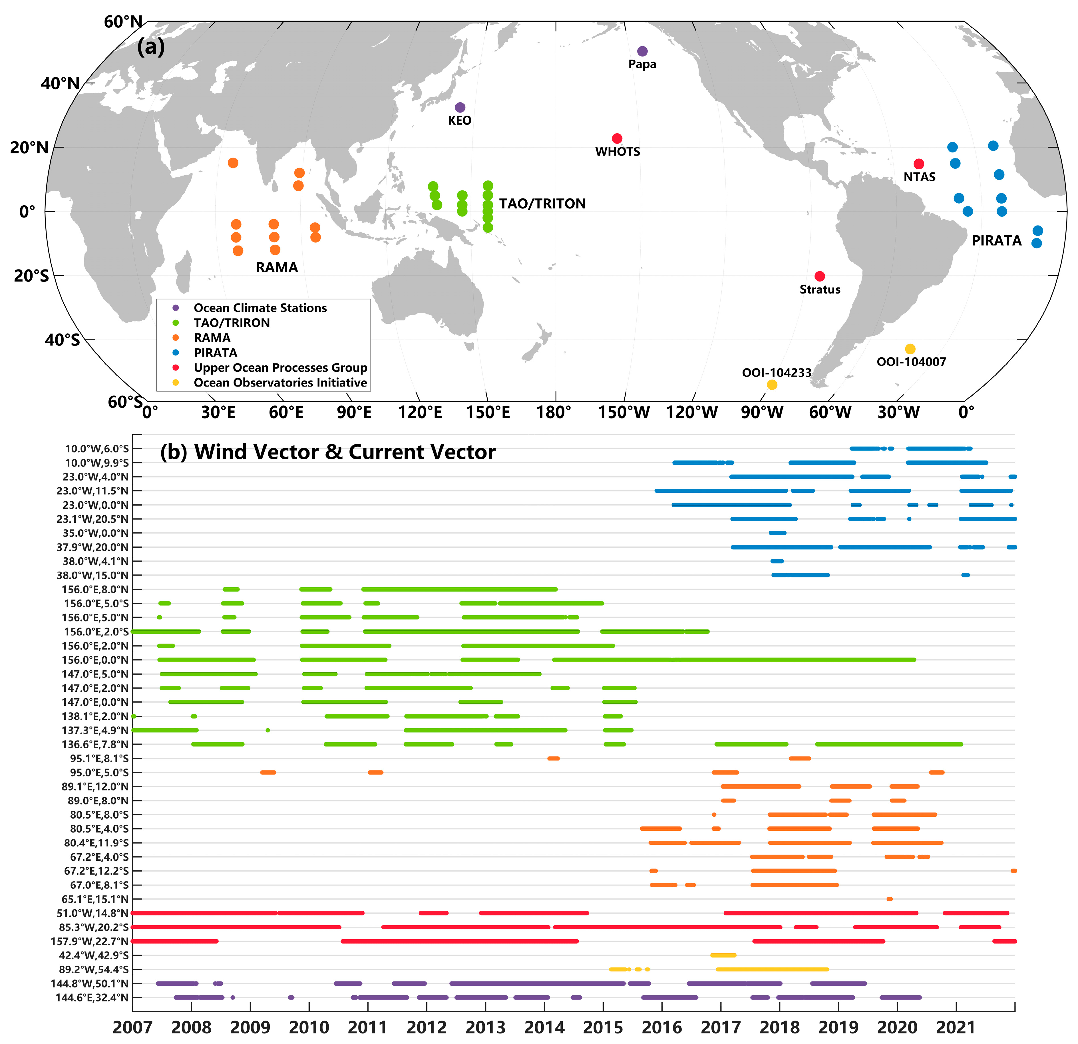
Figure 1. (a) The spatial distributions of the 40 moored buoys. (b) Timeline of hourly wind vector and current vector observations from these operational buoys. Distinct colors are utilized to denote moored buoy data acquired from various projects or organizations.
Remotesensing 15 04630 g001
Figure 2. (a) The number of data triplets that the ASCAT L2 wind vector matched with the moored buoy’s wind vector and current vector. (b) is the same as (a), but for the ASCAT L3 wind vector.
Remotesensing 15 04630 g002
Figure 3. (a) Multi-year averaged ocean surface current speed from 2007 to 2021. The gray arrows indicate the average current direction. (b) The probability density function (PDF) of the magnitude of the current speed, zonal component |u|, and meridional component |v|. (c) The PDF of the current direction and the angle between the current vector and wind vector.
Remotesensing 15 04630 g003
Figure 4. Comparisons of (a) the wind speed (WSPD), (b) the zonal and (c) meridional wind components between the buoy-based earth-relative observations and the collocated ASCAT L2 data. (df) are the same as (ac) but for the ASCAT L3 products. The color of each dot represents the density of the data. The number (n) of data pairs in each panel is noted in the title.
Remotesensing 15 04630 g004
Figure 5. The relationship between the ASCAT L2 wind bias and ocean surface velocity. The panels in each column represent differing buoys with all buoys on the left. The panels in each row represent the differing variables, with the scalar wind speed bias on the top. The bin-averaged wind bias with error bars as a function of the surface current is shown in each panel. The black dashed line provides the result from a linear regression fit, and the gray dashed line indicates a linear relationship with a slope of unity. The regression equation and the correlation coefficient (R) are noted in each panel. The number of data triplets and the distribution of the surface current speed are depicted in red shades.
Remotesensing 15 04630 g005
Figure 6. The same as Figure 5 but for the ASCAT L3 wind product.
Remotesensing 15 04630 g006
Figure 7. (ac) The correlation coefficients and (df) the slopes of the linear regression equation between the ASCAT L2 wind bias and the surface current velocity. (a,d) are for the scalar wind speed bias and projected current speed. (b,e) represent the zonal wind speed bias and surface velocity, while (c,f) correspond to the meridional component. Stations where the linear correlation does not pass the significance test at a 95% confidence level are labeled with gray triangles.
Remotesensing 15 04630 g007
Figure 8. The same as Figure 7 but for the ASCAT L3 wind product.
Remotesensing 15 04630 g008
Figure 9. Comparison of the ASCAT scalar wind speed and the buoy wind speed. The ASCAT wind speeds in (a,c) are uncorrected, while they have been corrected with surface current measured via moored buoys in (b,d). (ad) represent the results for the ASCAT L2 and L3 wind products, respectively. The color of the points indicates the projection of the ocean surface current onto the direction of the buoy-observed wind. The number (n) of data triplets in each panel is noted in the title.
Remotesensing 15 04630 g009
Figure 10. Comparisons of the zonal current u between the buoy observations and CMEMS reprocessing. Each subfigure represents data from different buoy stations, with the coordinates of each buoy indicated in the subfigure’s title. The color of each dot represents the density of the data. The number (n) of data pairs and the correlation coefficient (R) are noted in the top left corner of each panel. The units of bias and RMSEs are in meters per second (m/s).
Remotesensing 15 04630 g010
Figure 11. The same as Figure 10 but for the meridional current v .
Remotesensing 15 04630 g011
Figure 12. The same as Figure 9, but the reprocessed current is utilized for the correction of the ASCAT winds.
Remotesensing 15 04630 g012
Figure 13. The root-mean-square error of the ASCAT wind speed before and after correction using the ocean surface current. The corresponding percentages indicate the extent of the reduction in RMSE achieved.
Remotesensing 15 04630 g013
Table 1. The multi-year averaged coordinates of each buoy, along with the sensor types and deployment depths for ocean current measurements.
Buoy IDLongitudeLatitudeDepthSensor Type
KEO144.6°E32.4°N5 m, 6 m, 8 m, 11.5 m, 15 m, and 15.6 m at different deployment durationsSontek, TRDI Doppler volume sampler and Nortek Aquadopp current meter at different deployment durations
Papa144.8°W50.1°N5 m, 6 m, and 15 m at different deployment durationsSontek, TRDI Doppler Volume Sampler and Nortek Aquadopp Current Meter at different deployment durations
OOI-10423389.2°W54.4°S12 mSingle-point velocity meter
OOI-10400742.4°W42.9°S12 mSingle-point velocity meter
WHOI-WHOTS157.9°W22.7°N10 mVector measuring current meter
WHOI-Stratus85.3°W20.2°S7 m, 10 m, 13 m 15 m, and 20 m at different deployment durationsAanderaa ADCM, NORTEK ADCM, and Aanderaa RCM11 at different deployment durations
WHOI-NTAS51.0°W14.8°N5.7 m, 6 m, 12 m, and 13 m at different deployment durationsAquadopp current meter, NORTEK ADCM, and NORTEK current meter at different deployment durations
RAMA65.1°E15.1°N12 mSontek
67.0°E8.1°S
67.2°E12.2°S
67.2°E4.0°S
80.4°E11.9°S
80.5°E4.0°S
80.5°E8.0°S
89.0°E8.0°N
89.1°E12.0°N
95.0°E5.0°S10 m
95.1°E8.1°S
TAO/TRITON136.6°E7.8°N10 mSontek
137.3°E4.9°N
138.1°E2.0°N
147.0°E0.0°N
147.0°E2.0°N
147.0°E5.0°N
156.0°E0.0°N
156.0°E2.0°N
156.0°E2.0°S
156.0°E5.0°N
156.0°E5.0°S
156.0°E8.0°N
PIRATA38.0°W15.0°N12 mSontek
38.0°W4.1°N
37.9°W20.0°N
35.0°W0.0°N
23.1°W20.5°N
23.0°W0.0°N
23.0°W11.5°N
23.0°W4.0°N
10.0°W9.9°S
10.0°W6.0°S
Disclaimer/Publisher’s Note: The statements, opinions and data contained in all publications are solely those of the individual author(s) and contributor(s) and not of MDPI and/or the editor(s). MDPI and/or the editor(s) disclaim responsibility for any injury to people or property resulting from any ideas, methods, instructions or products referred to in the content.

