Analysis of Infrared Spectral Radiance of O₂ 1.27 μm Band Based on Space-Based Limb Detection

Abstract

The infrared spectral radiance of O₂ is of great significance for space-based infrared detection. In this work, based on the demand for near-infrared spectral radiance of O₂ limb detection, a method of spectral radiance calculation coupled with an atmospheric remote sensing model of limb detection is proposed. According to the selection criteria of fine spectral lines, the most suitable spectral lines of the O₂ 1.27 μm band for detection are given. Specifically, the limb infrared radiances of the O₂ 1.27 μm band were simulated by using the spectral line data from the spectral database, and the effects of molecular self-absorption were also considered. Furthermore, the infrared spectral radiance distribution of the O₂ 1.27 μm band was simulated under the influence of altitude, and finally, the detectability of the 1.27 μm band of O₂ molecules was analyzed using the criteria of spectral line selection, radiance intensity, spectral separation range and temperature sensitivity. The calculation results show that the spectral radiance of the 1.27 μm band of O₂ molecules first increases and then decreases with the decrease of the limb height, and the radiance reaches the peak value in the range of 40–50 km. In terms of the selection of spectral lines, the two groups of spectral lines R₇R₇, R₇Q₈ and R₁₁R₁₁, R₁₁Q₁₂ are most suitable for the limb detection and measurement of the O₂ 1.27 μm band.

1. Introduction

Wind field is an important physical quantity that characterizes the atmospheric state [1]. Current wind data can be widely obtained by ground-based detection [2] and indirect space-borne sensors [3]. However, these wind measurement methods are limited in both height coverage and temporal or spatial resolution. The continuous development of space measurement technology provides favorable conditions for space-borne wind temperature detection technology [4,5]. Space-borne airglow imaging interferometers adopt limb observation and can detect atmospheric wind fields and temperature fields on a global scale by detecting frequency shifts and intensity changes of the airglow spectral line, and they have become the forefront of the international satellite remote sensing field [6]. For wind field detection, the accuracy of wind field detection depends on the fine measurement of the spectral lines of specific components in the atmosphere [7]. In order to improve the accuracy of wind field measurements, the spectral lines of specific atmospheric components need to be analyzed, and fine spectral lines suitable for detection should be selected from numerous spectral lines. In the composition of the earth’s atmosphere, the infrared radiance of O₂ is strong, and the height coverage is wide, which provides an important means for remote sensing of the composition structure and dynamics of the global upper atmosphere [8].

At present, the atmospheric measurement and analysis of O₂ are widely used in wind field measurements. For near-infrared space-based detection, the instruments currently in orbit focus on the O₂ absorption band of 0.76 μm [9] and the CO₂/CH₄ absorption bands of 1.6 μm and 2.0 μm [8]. The O₂ 0.76 μm band has traditionally been used for satellite remote sensing [10], including the SCanning Imaging Absorption spectroMeter for Atmospheric CHartographY (SCIAMACHY) [11], the Greenhouse gas Observing SATellite (GOSAT) [12], the Orbiting Carbon Observatory-2 (OCO-2) [13], and others. However, the O₂(a¹Δ) band near 1.27 μm may be an optimal choice, with the wavelength of O₂ (a¹Δ) being closer to the CO₂ absorption band, which reduces the uncertainty associated with spectral changes in the atmospheric path [14]. In addition, the absorption lines are weaker than those in the 0.76 μm band, so the radiative transfer modeling is more accurate. Jean-Loup Bertaux et al. studied the O₂ absorption band for greenhouse gas monitoring and microcarb applications, indicating the presence of another, weaker O₂ absorption band at 1.27 μm [15]. Since the wavelength is closer to the CO₂ and CH₄ bands, there is less uncertainty when using it as a proxy for the atmospheric path length of the CO₂ and CH₄ bands. In addition, the reduced spectral spacing may also enable a simpler instrument design and potentially reduce the cost of the payload. It has been pointed out that O₂ radiance can be completely separated from sunlight without a significant loss of precision and accuracy [16]. Meanwhile, the O₂ 0.76 μm band is stronger and mostly saturated compared to the CO₂/CH₄ band, while the O₂ 1.27 μm band is weaker and able to maintain sensitivity over a wider range [15]. Therefore, the use of the O₂ 1.27 μm band for detection can meet various requirements, such as atmospheric wind field detection and temperature detection.

Currently, there are many measurement experiments for the detection of the O₂ 1.27 μm band’s infrared spectral radiance. Total Carbon Column Observing Network (TCCON) [17] used the O₂ 1.27 μm band instead of the 0.76 μm band to calculate the CO₂/dry-air mix ratio [18]; WAves Michelson Interferometer (WAMI) measures the O₃ concentration, rotation temperature, and O₂ airglow from 45 to 95 km, and it proposed two sets observation lines, one strong and one weak, to measure the O₂ 1.27 μm band radiance [19]. The Doppler Asymmetric Spatial Heterodyne-spectroscopy (DASH) instrument was used to measure the O₂ 1.27 μm limb radiance [16]. It has been proposed that the emission line of O₂ O₁₉P₁₈ (7772.030 cm⁻¹) be used as the target source for wind field detection [20]. However, current research on the O₂ 1.27 μm band mainly focuses on experimental infrared observation for the detection of greenhouse gases such as CO₂/CH₄, etc. For wind field detection, there is a lack of a fine spectral line selection model. In order to improve the measurement accuracy of wind field detection, it is necessary to analyze the spectral lines of the O₂ 1.27 μm band accurately to determine the spectral line with the best detection effect.

Focused on the need for a fine spectral line selection for the limb infrared detection of the O₂ 1.27 μm band, this paper combined spectral radiance calculation with an atmospheric remote sensing model to simulate the limb spectral radiance of the O₂ 1.27 μm band and to select the most suitable spectral line for detection. Firstly, the spectral lines of the O₂ 1.27 μm band were obtained through the HIgh-resolution TRANsmission molecular absorption database (HITRAN). Then, the self-absorption effect of the O₂ 1.27 μm band was analyzed. Then, the spectral radiance of O₂ 1.27 μm on the limb observation path was simulated by the line-by-line method, the spectral lines were selected according to the selection criteria of spectral lines, and the spectral lines with the best detection effect were obtained. In Section 2, the radiance characteristics of the earth’s spectral lines for O₂ 1.27 μm and the calculation method for the spectral radiation characteristics of the edge are introduced. In Section 3, the spectral radiance of limb detection, which varies with height, is calculated by the line-by-line method, and the spectral lines are screened according to the selection criteria. Section 4 is the conclusion of this paper.

2. Data and Methods

The photochemical interaction and spectral emission transition mechanism have become important factors that affect the detection of O₂ in the atmospheric wind field [21]. The infrared atmospheric spectral information and radiation characteristics determine the theoretical design of the detector observing the O₂ infrared atmospheric band and the accuracy of the radiation model for calculating the emission spectrum of the O₂(a¹Δ) → O₂(X³Σ) band [22]. Figure 1 shows the schematic diagram of O₂ limb detection, where $I_0$ represents the initial radiance, and $l_n$ represents the length of the nth layer.

2.1. O₂ (a¹Δ) Emission in the Earth’s Atmosphere

In the earth’s atmosphere, the emission radiance in the near infrared region at 1.27 µm occurs when molecular oxygen in its first excited electronic state O₂(a¹Δ) spontaneously relaxes to its fundamental state O₂(X³Σ). This is the source of oxygen molecular radiation at the 1.27 μm band [15]. Figure 2 shows the schematic diagram of the photochemical processes of O₂ in the earth’s atmosphere, where $J$ represents solar photolysis, $k$ represents collisional quenching, $A$ represents spontaneous emission, and $g$ represents solar excitation.

The radiance in the 1.27 μm band of the oxygen molecule results from the spontaneous emission and collisional quenching generated by the first excited state O₂(a¹Δ). The spontaneous emission process A_Δ is as follows:

$$A_{\Delta }:{ \mathrm{O}}_2\left({\mathrm{a}}^1\Delta \right) \to { \mathrm{O}}_2({\mathrm{X}}^3\Sigma )+h\nu \left(1.27 \mathsf{\mu }\mathrm{m}\right)$$

(1)

The collisional quenching of O₂(a¹Δ) can be performed with O₂, N₂, O, O₃, or CO₂. Of these, collisions with O₂ k_Δ dominate the earth’s atmosphere [24]:

$$k_{\Delta }:{ \mathrm{O}}_2\left({\mathrm{a}}^1\Delta \right)+ \mathrm{M}\to {\mathrm{O}}_2\left({\mathrm{X}}^3\Sigma \right)+ \mathrm{M}$$

(2)

The main direct source of the formation of O₂(a¹Δ) is the photo-dissociation of O₃ at wavelengths shorter than 310 nm in the earth’s atmosphere. The photo-dissociation of O₃ produces molecules of O₂ in the electronic state O₂(a¹Δ) and oxygen atoms of O in the excited state O(¹D) [25]:

$$J_H:{ \mathrm{O}}_3+h\nu \left(\lambda <310 \mathrm{nm}\right)\to {\mathrm{O}}_2\left({\mathrm{a}}^1\Delta \right)+ \mathrm{O}\left({}^1\mathrm{D}\right)$$

(3)

The processes of photo-dissociation also include Schumann–Runge continuum J_SRC and J_Ly-α. However, this is not taken into account in this article, since it only represents about 1% of the integrated emission [15].

Another direct production process of O₂(a¹Δ) is the recombination of oxygen atoms in their fundamental state O(³P). However, since this production of O₂(a¹Δ) is mainly generated in the upper atmosphere and contributes little to O₂ radiance, it will be neglected here.

Another source of O₂(a¹Δ) is the indirect production by O(¹D). Once O(¹D) is formed by the photo-dissociation of ozone occurring at the rate J_H, its relaxation towards O(³P) occurs in spontaneous emission A_D and collisional quenching k_D. The spontaneous emission A_D leads to the emission of a photon at 630 nm, and the collisional quenching O(¹D) can be performed with N₂ or O₂:

$$A_{\mathrm{D}}: \mathrm{O}\left({}^1\mathrm{D}\right)\to \mathrm{O}\left({}^3\mathrm{P}\right)+h\nu \left(630 \mathrm{nm}\right)$$

(4)

$$k_{{\mathrm{D},\mathrm{N}}_2}: \mathrm{O}\left({}^1\mathrm{D}\right)+{ \mathrm{N}}_2\to \mathrm{O}\left({}^3\mathrm{P}\right)+{ \mathrm{N}}_2$$

(5)

$$k_{{\mathrm{D},\mathrm{O}}_2}: \mathrm{O}\left({}^1\mathrm{D}\right){+\mathrm{O}}_2\to \mathrm{O}\left({}^3\mathrm{P}\right){+\mathrm{O}}_2\left({\mathrm{b}}^1\mathsf{\Sigma }\right)$$

(6)

The collisional quenching process k_D,O2 in which O₂ participates produces O₂ in its second excited state O₂(b¹Σ). This unstable molecule O₂(b¹Σ) relaxes into the fundamental state O₂(X³Σ) after spontaneous emission A_Σ and is accompanied by emission radiance at 762 nm. Meanwhile, the collisional quenching k_Σ of O₂(b¹Σ) can be performed with O, O₂, O₃, N₂, and CO₂, and it results in the first excited state O₂(a¹Δ) [26]:

$$A_{\Sigma }:{ \mathrm{O}}_2\left({\mathrm{b}}^1\Sigma \right) \to { \mathrm{O}}_2\left({\mathrm{X}}^3\Sigma \right)+h\nu \left(762 \mathrm{nm}\right)$$

(7)

$$k_{\mathsf{\Sigma },\mathrm{O}}:{ \mathrm{O}}_2\left({\mathrm{b}}^1\mathsf{\Sigma }\right)+ \mathrm{M} \to { \mathrm{O}}_2\left({\mathrm{a}}^1\mathsf{\Delta }\right)+ \mathrm{M}$$

(8)

In these processes, the absorption by the fundamental state O₂(X³Σ) of the solar radiance at 762 nm raises it to its second excited state O₂(b¹Σ):

$$g_{\mathrm{O}}{}_{{}_2}:{ \mathrm{O}}_2\left({\mathrm{X}}^3\mathsf{\Sigma }\right)+h\nu \left(762\mathrm{nm}\right) \to { \mathrm{O}}_2\left({\mathrm{b}}^1\mathsf{\Sigma }\right)$$

(9)

The second excited state O₂(b¹Σ) produced by the previous process is then affected by the same processes, which in the case of quenching lead to the O₂(a¹Δ) state. These processes form the theoretical basis of the O₂(a¹Δ) emission model.

2.2. O₂ Limb Spectral Radiance

In order to accurately simulate the limb infrared spectral radiance characteristics of the O₂ 1.27 μm band and determine the best spectral line for detection, the line-by-line method was used to simulate the infrared spectral radiation of an O₂ molecule in the 1.27 μm band. At present, the line-by-line method is the most accurate method for calculating the absorption coefficient, and it has a high resolution and is appropriate for fine spectral line analysis [27]. Therefore, in this paper, the line-by-line method is used to calculate the limb infrared spectral radiance of O₂ at the 1.27 μm band.

It is necessary to obtain the atmospheric parameters of the target region in order to calculate the spectral radiance through the line-by-line method. After determining the thermodynamic state of the target region, including temperature T and pressure P, the absorption coefficient $k_{\nu }\left(P,T\right)$ can be expressed as:

$$k_{\nu }\left(P,T\right)=N_0(\frac{T_{0}P}{T{P}_0}){\displaystyle \sum _{j=1}^n{S}_{\nu ,j}\left(T\right)f_{\nu ,j}\left(P,T\right)}$$

(10)

where $\nu$ is the spectral frequency, $N_0$ is the number density under the reference state (temperature $T_0$, pressure $P_0$), $S_{\nu ,j}(T)$ is the spectral line intensity at temperature T, $f_{\nu ,j}(P,T)$ is the normalized spectral line linear function, and n is the total number of spectral lines. In order to calculate the spectral line intensity $S_{\nu ,j}(T)$ at temperature T, it is necessary to obtain the spectral line intensity $S_{\nu ,j}(T_0)$ under the reference temperature T₀ through the HITRAN database [28]. The $S_{\nu ,j}(T)$ can be calculated according to the following equation:

$$S_{\nu ,j}\left(T\right)=S_{\nu ,j}\left(T_0\right)\frac{Q_{tot}(T_0)}{Q_{tot}(T)}\exp \left[-c_{2}E\left(\frac{1}{T}-\frac{1}{T_0}\right)\right]\frac{\left[1-\exp \left(-c_2\nu /T\right)\right]}{\left[1-\exp \left(-c_2\nu /T_0\right)\right]}$$

(11)

where $c_2=hc/k$ is the second radiation constant, $Q_{tot}\left(T\right)$ is the total partition function at the reference temperature, and E is the energy of the low-level state. The HITRAN database is the most commonly used source of reference molecular spectroscopic data for molecules of atmospheric interest. In this work, the 1.27 μm band line for an oxygen molecule was obtained from HITRAN on the Web. Figure 3 shows the O₂ 1.27 μm spectral line at 296 K found in HITRAN data [29], where P, Q, R represent the set of “local” quantum numbers for upper and lower rotational states.

The normalized spectral line linear function $f_{\nu ,j}(P,T)$ used in this paper is the Voigt broadening linear function. Voigt broadening is the most commonly used spectral line broadening [30]:

$$f_V\left(\nu -{\nu }_0\right)=\frac{{\alpha }_L}{{\pi }^{3/2}}{\displaystyle {\int }_{-\infty }^{+\infty }\frac{\exp (-x^2)}{{\left(\nu -{\nu }_0-x{\alpha }_D/\sqrt{\ln 2}\right)}^2+{\alpha }_L^2}dx}$$

(12)

where ${\alpha }_L$ is the Lorentz half width, and ${\alpha }_D$ is the Doppler half width. The Lorentz half-width ${\alpha }_L$ is expressed as [27]:

$${\alpha }_L=\left[\left(1-x\right){\gamma }_{air}+x{\gamma }_{self}\right]P{\left(\frac{T_0}{T}\right)}^{n_{air}}$$

(13)

where $x$ is the partial pressure ratio, ${\gamma }_{air}$ is the broadening caused by air, ${\gamma }_{self}$ is the line’s self-broadening, and $n_{air}$ is the temperature dependence coefficient; the Doppler half width ${\alpha }_D$ is expressed as [31]:

$${\alpha }_D=\frac{v_0}{c}\sqrt{\frac{2kT}{M}\ln 2}$$

(14)

where M is the mass of a single molecule. The monochromatic transmittance ${\tau }_{\nu }$ obtained by integrating the path l from s = 0 to s = s₁ is expressed as:

$${\tau }_{\nu }=\exp [-{\displaystyle {\int }_0^{s_1}{k}_{\nu }(P,T)ldl}]$$

(15)

According to Beer–Lambert’s law, the radiance intensity $I_{\nu }$ at the end of the path $s_1$ is expressed as:

$$I_{\nu }=I_B(1-{\tau }_{\nu })$$

(16)

where $I_B$ is the radiance of Blackbody radiation. Formulas (10)–(16) represent the calculation method of spectral radiance when the path is a single-layer homogeneous medium. However, in the process of limb detection, the non-uniformity of the atmospheric profile will lead to error in the calculation of the absorption coefficient. At the same time, the molecular transition radiates photons, and the photons will be re-absorbed by the same kinds of particles in the ground state during the propagation process, which is the self-absorption effect of photons [20]. Under the optical thin hypothesis, the self-absorption effect of photons can usually be ignored. However, in practice, the optical thin hypothesis is not valid in research objects such as combustion and plasma, and the self-absorption effect will lead to changes in the structure of the emission spectrum. The self-absorption effect should be considered in the calculation of line-of-sight integration. The spectral radiance of each layer is determined by the atmospheric parameters of that layer. Considering the molecular self-absorption effect, the spectral radiance of multilayer gas is:

$$I=\left\{\begin{array}{l}{I}_0{e}^{-{\displaystyle \sum _{m=1}^N{k}_m\cdot l_m}}+{\displaystyle \sum _{n=2}^N\left[I_{n-1}(1-e^{-k_{n-1}\cdot l_{n-1}})e^{-{\displaystyle \sum _{j=n}^N{k}_j\cdot l_j}}\right]}\hspace{0.33em}\hspace{0.33em}(\mathrm{with}\hspace{0.33em}\mathrm{self}-\mathrm{absorption})\\ I_0+{\displaystyle \sum _{n=1}^N{I}_n{e}^{-k_n\cdot l_n}}\hspace{0.33em}\hspace{0.33em}\hspace{0.33em}\hspace{0.33em}\hspace{0.33em}\hspace{0.33em}\hspace{0.33em}\hspace{0.33em}\hspace{0.33em}\hspace{0.33em}\hspace{0.33em}\hspace{0.33em}\hspace{0.33em}\hspace{0.33em}\hspace{0.33em}\hspace{0.33em}\hspace{0.33em}\hspace{0.33em}\hspace{0.33em}\hspace{0.33em}(\mathrm{without}\hspace{0.33em}\mathrm{self}-\mathrm{absorption})\end{array}\right.$$

(17)

where I_n is the emission radiance of the nth layer, k_n is the absorption coefficient of the nth layer, and l_n is the path length of the nth layer.

Figure 4 shows the infrared spectral radiance of the O₂ 7870 cm⁻¹ band for the same path length (100 km) at a tangent height of 90–20 km and shows the contrast of spectral line brightness with and without the effect of self-absorption. As shown in Figure 5, in the height range above 60 km, self-absorption has little effect on spectral radiance, while in the range below 50 km, the effect is significant, and the phenomenon of self-absorption increases with a decrease of the tangential height. At the same time, the self-absorption phenomenon is very obvious in most of the Q-branch infrared atmospheric band with the highest radiation peak, which makes it difficult to use this band in many applications with a low tangent height.

3. Results and Discussion

As shown in Figure 5, according to Equations (10)–(17), the limb infrared spectral radiance of O₂ at the limb height of 10–90 km was simulated, with the observed height being 100 km. The atmospheric parameters are based on the 1976 US Standard Atmospheric Model [32]. Figure 5 shows that with the decrease of the limb height, the O₂ spectral radiance of the 7870 cm⁻¹ band first increases and then decreases, and the peak radiance exceeds 4.5 × 10⁻¹⁶ (W/m²·sr·cm⁻¹) at 40–50 km. Above 60 km, the spectral radiance of O₂ is lower because the molar fraction of O₂ in the upper atmosphere is low, and the limb observation path is too long. Below 20 km, due to the strong self-absorption effect of the molecules, the spectral radiance of O₂ is reduced.

Although the results show that the oxygen molecule has multiple bright spectral lines in the 7870 cm⁻¹ band, the lines in the band are closely spaced and therefore difficult to cleanly isolate. These issues can be overcome through the spectral line selection. The spectral lines that are suitable for detection are selected by the following criteria:

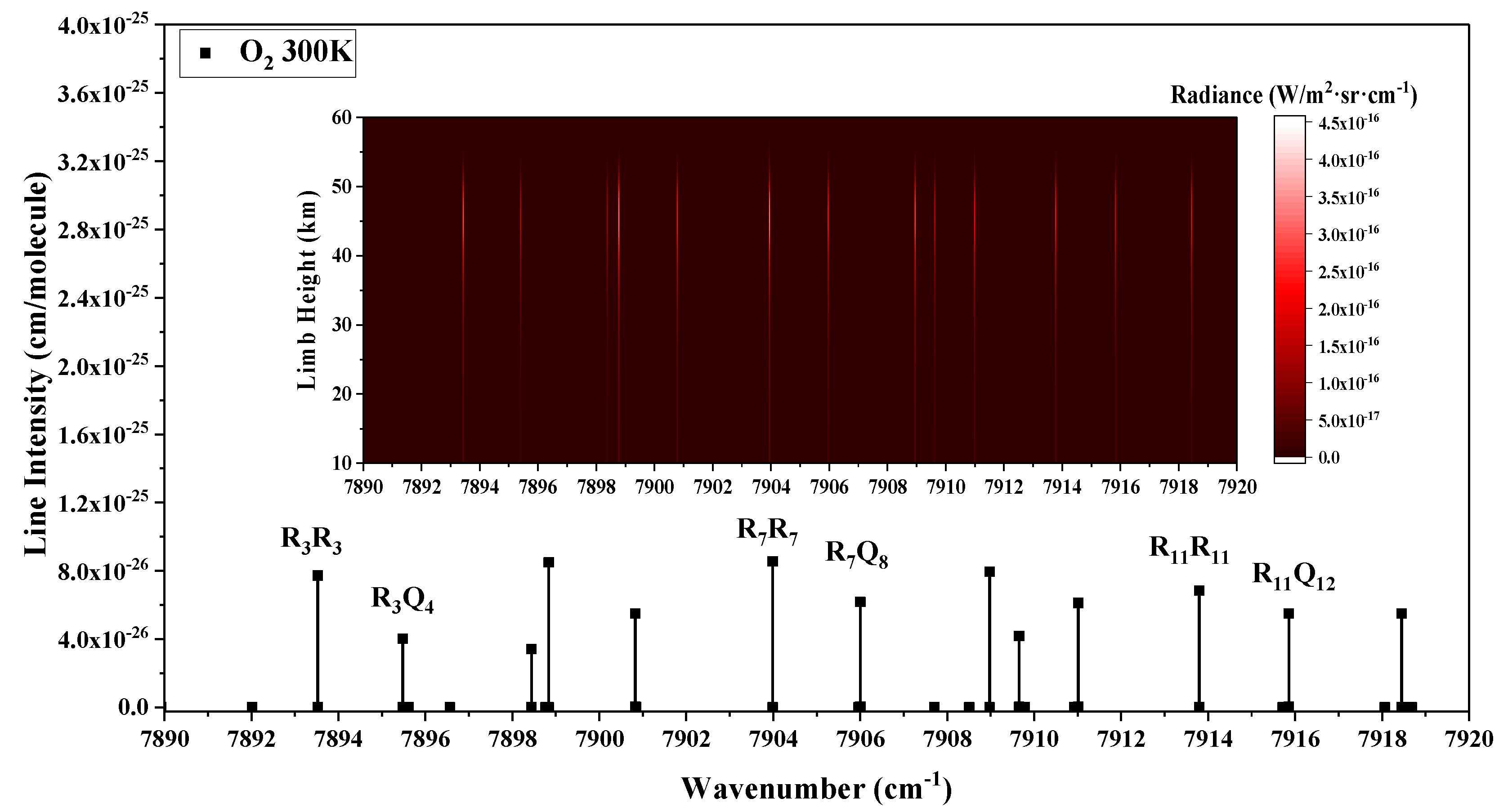
• The separation of spectral lines. There are thousands of molecular spectral lines, and the distribution is relatively dense; thus, it is necessary to select spectral lines with a better separation, so that the optical system can separate the target spectral lines [19]. They are relatively well separated from the neighboring lines, with a distance of more than 0.4 nm.
• The temperature sensitivity. It is necessary to select a group comprised of several spectral lines located in close proximity and with different temperature sensitivities to ensure the sensitivity of the spectral line intensity ratio to temperature [7]. Among these, spectral lines with a weak temperature sensitivity are used for the calibration of atmospheric parameters to determine the accuracy of measurement, and spectral lines with a strong temperature sensitivity are used for temperature inversion and atmospheric parameter measurements, with high sensitivity.

As shown in Figure 6, the spectral lines with a strong radiance in the results were selected for spectral line separation; there were three groups of spectral lines with a strong radiation intensity and high spectral line separation, namely group R₃R₃ (7893.528299 cm⁻¹), R₃Q₄ (7895.477867 cm⁻¹), group R₇R₇ (7903.988200 cm⁻¹), R₇Q₈ (7906.004087 cm⁻¹), and group R₁₁R₁₁ (7913.794638 cm⁻¹), R₁₁Q₁₂ (7915.856069 cm⁻¹). These three groups of spectral lines can be used as measured spectral lines with a distance greater than 0.4 nm from the neighboring spectral lines, and they can be used as measured spectral lines under the conditions of satisfying the radiance intensity and spectral line separation.

The temperature sensitivity of the selected spectral lines is shown in Figure 7. Among them, the group R₃R₃, R₃Q₄ and group R₇R₇, R₇Q₈ bands and two groups of lines have a strong temperature sensitivity, while the group R₁₁R₁₁, R₁₁Q₁₂ bands have a weak temperature sensitivity. However, considering the self-absorption effect of molecules, R₃R₃, R₃Q₄ is closer to the Q branch spectral line in the center of the 7870 cm⁻¹ band, and the self-absorption effect is stronger, resulting in a narrow height application range. Therefore, the most suitable spectral lines for detection are group R₇R₇, R₇Q₈ and group R₁₁R₁₁, R₁₁Q₁₂.

4. Conclusions

Based on the need to detect the limb infrared spectral radiance characteristics of O₂ in the 1.27 μm band, a method of spectral radiance calculation coupled with an atmospheric remote sensing model of limb detection is proposed, which can effectively simulate the spectral radiance distribution of the atmospheric composition. According to the criteria of fine spectral line selection, the O₂ spectral line of the 1.27 μm band is selected. In this paper, the absorption coefficient of O₂ spectral lines obtained from the HITRAN database is calculated by using the line-by-line method. Then, the atmospheric path is stratified by the limb atmospheric model, and the infrared spectral radiance of the 1.27 μm band of O₂ is calculated by the LOS method. The spectral radiance distribution for 10–90 km is calculated. The results show that the spectral radiance of the O₂ 1.27 μm band first increases and then decreases with the decrease of limb height, and the peak radiance exceeds 4.5 × 10⁻¹⁶(W/m²·sr·cm⁻¹) at 40–50 km. After considering the radiation intensity, spectral line separation, and temperature sensitivity, it is shown that the group R₇R₇, R₇Q₈ and group R₁₁R₁₁, R₁₁Q₁₂ spectral lines in the O₂ 1.27 μm band are the most suitable for the limb detection. Among them, group R₇R₇, R₇Q₈ has a strong temperature sensitivity and can be used for temperature inversion and atmospheric parameter measurements, with a high sensitivity, and group R₁₁R₁₁, R₁₁Q₁₂ has a weak temperature sensitivity and can be used for the calibration of atmospheric parameters to determine the accuracy of measurements.

References

1. Han, Y.; Sun, D.; Han, F.; Liu, H.; Zhao, R.; Zhen, J.; Zhang, N.; Chen, C.; Li, Z. Demonstration of daytime wind measurement by using mobile Rayleigh Doppler Lidar incorporating cascaded Fabry-Perot etalons. Opt. Express 2019, 27, 34230–34246. [Google Scholar] [CrossRef]
2. Baumgarten, G. Doppler Rayleigh/Mie/Raman lidar for wind and temperature measurements in the middle atmosphere up to 80 km. Atmos. Meas. Tech. 2010, 3, 1509–1518. [Google Scholar] [CrossRef]
3. Mitra, A.K.; Kundu, P.K.; Giri, R.K. A quantitative analysis of KALPANA-1 derived water vapor winds and its impact on NWP model. Meteorol. Atmos. Phys. 2013, 120, 29–44. [Google Scholar] [CrossRef]
4. Šavli, M.; Kloe, J.; Marseille, G.J.; Rennie, M.; Žagar, N.; Wedi, N. The prospects for increasing the horizontal resolution of the Aeolus horizontal line-of-sight wind profiles. Q. J. R. Meteorol. Soc. 2019, 145, 3499–3515. [Google Scholar] [CrossRef]
5. Shepherd, G.G. Development of wind measurement systems for future space missions. Acta Astronaut. 2015, 115, 206–217. [Google Scholar] [CrossRef]
6. Englert, C.R.; Harlander, J.M.; Brown, C.M.; Marr, K.D.; Miller, I.J.; Stump, J.E.; Hancock, J.; Peterson, J.Q.; Kumler, J.; Morrow, W.H.; et al. Michelson Interferometer for Global High-resolution Thermospheric Imaging (MIGHTI): Instrument Design and Calibration. Space Sci. Rev. 2017, 212, 553–584. [Google Scholar] [CrossRef] [PubMed]
7. Kassi, S.; Guessoum, S.; Abanto, J.C.A.; Tran, H.; Campargue, A.; Mondelain, D. Temperature Dependence of the Collision-Induced Absorption Band of O2 Near 1.27 µm. J. Geophys. Res. Atmos. 2021, 126, e2021JD034860. [Google Scholar] [CrossRef]
8. Boesche, E.; Stammes, P.; Bennartz, R. Aerosol influence on polarization and intensity in near-infrared O2 and CO2 absorption bands observed from space. J. Quant. Spectrosc. Radiat. Transf. 2009, 110, 223–239. [Google Scholar] [CrossRef]
9. Tran, H.; Hartmann, J.M. An improved O2 A band absorption model and its consequences for retrievals of photon paths and surface pressures. J. Geophys. Res. 2008, 113, 18104. [Google Scholar] [CrossRef]
10. Drouin, B.J.; Benner, D.C.; Brown, L.R.; Cich, M.J.; Crawford, T.J.; Devi, V.M.; Guillaume, A.; Hodges, J.T.; Mlawer, E.J.; Robichaud, D.J.; et al. Multispectrum analysis of the oxygen A-band. J. Quant. Spectrosc. Radiat. Transf. 2017, 186, 118–138. [Google Scholar] [CrossRef]
11. de Laat, A.T.J.; Gloudemans, A.M.S.; Aben, I.; Schrijver, H. Global evaluation of SCIAMACHY and MOPITT carbon monoxide column differences for 2004–2005. J. Geophys. Res. 2010, 115, D06307. [Google Scholar] [CrossRef]
12. Butz, A.; Guerlet, S.; Hasekamp, O.; Schepers, D.; Galli, A.; Aben, I.; Frankenberg, C.; Hartmann, J.M.; Tran, H.; Kuze, A.; et al. Toward accurate CO2 and CH4observations from GOSAT. Geophys. Res. Lett. 2011, 38, L14812. [Google Scholar] [CrossRef]
13. Jung, Y.; Kim, J.; Kim, W.; Boesch, H.; Lee, H.; Cho, C.; Goo, T.-Y. Impact of Aerosol Property on the Accuracy of a CO2 Retrieval Algorithm from Satellite Remote Sensing. Remote Sens. 2016, 8, 322. [Google Scholar] [CrossRef]
14. Sun, K.; Gordon, I.E.; Sioris, C.E.; Liu, X.; Chance, K.; Wofsy, S.C. Reevaluating the Use of O2 a1Δg Band in Space borne Remote Sensing of Greenhouse Gases. Geophys. Res. Lett. 2018, 45, 5779–5787. [Google Scholar] [CrossRef]
15. Bertaux, J.-L.; Hauchecorne, A.; Lefèvre, F.; Bréon, F.-M.; Blanot, L.; Jouglet, D.; Lafrique, P.; Akaev, P. The use of the 1.27 µm O2 absorption band for greenhouse gas monitoring from space and application to MicroCarb. Atmos. Meas. Tech. 2020, 13, 3329–3374. [Google Scholar] [CrossRef]
16. He, W.; Hu, X.; Wang, H.; Wang, D.; Li, J.; Li, F.; Wu, K. Influence of Scattered Sunlight for Wind Measurements with the O2(a1Δg) Dayglow. Remote Sens. 2022, 15, 232. [Google Scholar] [CrossRef]
17. Wunch, D.; Toon, G.C.; Blavier, J.F.; Washenfelder, R.A.; Notholt, J.; Connor, B.J.; Griffith, D.W.; Sherlock, V.; Wennberg, P.O. The total carbon column observing network. Philos. Trans. A Math. Phys. Eng. Sci. 2011, 369, 2087–2112. [Google Scholar] [CrossRef]
18. Jacob, D.J.; Turner, A.J.; Maasakkers, J.D.; Sheng, J.; Sun, K.; Liu, X.; Chance, K.; Aben, I.; McKeever, J.; Frankenberg, C. Satellite observations of atmospheric methane and their value for quantifying methane emissions. Atmos. Chem. Phys. 2016, 16, 14371–14396. [Google Scholar] [CrossRef]
19. Fujisada, H.; Ward, W.E.; Lurie, J.B.; Gault, W.A.; Shepherd, G.G.; Weber, K.; Rowlands, N. Waves Michelson Interferometer: A visible/near-IR interferometer for observing middle atmosphere dynamics and constituents. In Sensors, Systems, and Next-Generation Satellites V; Society of Photo Optical: Bellingham, WA, USA, 2001. [Google Scholar]
20. Wu, K.; Fu, D.; Feng, Y.; Li, J.; Hao, X.; Li, F. Simulation and application of the emission line O19P18 of O2(a1Δg) dayglow near 1.27 mum for wind observations from limb-viewing satellites. Opt. Express 2018, 26, 16984–16999. [Google Scholar] [CrossRef]
21. He, W.; Wu, K.; Feng, Y.; Fu, D.; Chen, Z.; Li, F. The Radiative Transfer Characteristics of the O2 Infrared Atmospheric Band in Limb-Viewing Geometry. Remote Sens. 2019, 11, 2702. [Google Scholar] [CrossRef]
22. Mondelain, D.; Kassi, S.; Campargue, A. Accurate Laboratory Measurement of the O2 Collision-Induced Absorption Band Near 1.27 μm. J. Geophys. Res. Atmos. 2019, 124, 414–423. [Google Scholar] [CrossRef]
23. Yankovsky, V.; Manuilova, R.; Babaev, A.; Feofilov, A.; Kutepov, A. Model of electronic-vibrational kinetics of the O3 and O2 photolysis products in the middle atmosphere: Applications to water vapour retrievals from SABER/TIMED 6.3 μm radiance measurements. Int. J. Remote Sens. 2011, 32, 3065–3078. [Google Scholar] [CrossRef]
24. Zarboo, A.; Bender, S.; Burrows, J.P.; Orphal, J.; Sinnhuber, M. Retrieval of O2(1Σ) and O2(1Δ) volume emission rates in the mesosphere and lower thermosphere using SCIAMACHY MLT limb scans. Atmos. Meas. Tech. 2018, 11, 473–487. [Google Scholar] [CrossRef]
25. Martyshenko, K.V.; Yankovsky, V.A. IR band of O2 at 1.27 μm as the tracer of O3 in the mesosphere and lower thermosphere: Correction of the method. Geomagn. Aeron. 2017, 57, 229–241. [Google Scholar] [CrossRef]
26. Yee, J.-H.; DeMajistre, R.; Morgan, F. The O2(b1Σ) dayglow emissions: Application to middle and upper atmosphere remote sensing1This article is part of a Special issue that honours the work of Dr. Donald M. Hunten FRSC who passed away in December 2010 after a very illustrious career. Can. J. Phys. 2012, 90, 769–784. [Google Scholar] [CrossRef]
27. Coelho, F.R.; Ziemniczak, A.; Roy, S.P.; França, F.H.R. A new line-by-line methodology based on the spectral contributions of the bands. Int. J. Heat Mass Transf. 2021, 164, 120423. [Google Scholar] [CrossRef]
28. Gordon, I.E.; Rothman, L.S.; Hargreaves, R.J.; Hashemi, R.; Karlovets, E.V.; Skinner, F.M.; Conway, E.K.; Hill, C.; Kochanov, R.V.; Tan, Y.; et al. The HITRAN2020 molecular spectroscopic database. J. Quant. Spectrosc. Radiat. Transf. 2022, 277, 107949. [Google Scholar] [CrossRef]
29. Kochanov, R.V.; Gordon, I.E.; Rothman, L.S.; Shine, K.P.; Sharpe, S.W.; Johnson, T.J.; Wallington, T.J.; Harrison, J.J.; Bernath, P.F.; Birk, M.; et al. Infrared absorption cross-sections in HITRAN2016 and beyond: Expansion for climate, environment, and atmospheric applications. J. Quant. Spectrosc. Radiat. Transf. 2019, 230, 172–221. [Google Scholar] [CrossRef]
30. Humlicek, J. Reprint of: Optimized computation of the voigt and complex probability functions. J. Quant. Spectrosc. Radiat. Transf. 2010, 111, 1545–1552. [Google Scholar]
31. Schreier, F. The Voigt and complex error function: A comparison of computational methods. J. Quant. Spectrosc. Radiat. Transf. 1992, 48, 743–762. [Google Scholar] [CrossRef]
32. Berk, A.; Hawes, F. Validation of MODTRAN®6 and its line-by-line algorithm. J. Quant. Spectrosc. Radiat. Transf. 2017, 203, 542–556. [Google Scholar] [CrossRef]
Figure 1. Schematic diagram of O2 space-based limb detection.
Remotesensing 15 04648 g001
Figure 2. Schematic diagram of the photochemical processes of O2 in the earth’s atmosphere [23]. (The left axis represents the wavenumber generated by the molecular transition, and the right axis represents the energy of the molecule in that energy state).
Remotesensing 15 04648 g002
Figure 3. O2 1.27 μm spectral line intensity at 296 K found in HITRAN data.
Remotesensing 15 04648 g003
Figure 4. The simulated spectral radiance of the O2 7870 cm−1 band at a tangent height of 90–20 km (with and without the effect of self-absorption).
Remotesensing 15 04648 g004
Figure 5. The spectral radiance distribution of O2 7870 cm−1 band with the limb height.
Remotesensing 15 04648 g005
Figure 6. Spectral lines that can be detected considering spectral line separation (greater than 0.4 nm). (Group R3R3, R3Q4, group R7R7, R7Q8, and group R11R11, R11Q12).
Remotesensing 15 04648 g006
Figure 7. Distribution of O2 spectral lines with temperature.
Remotesensing 15 04648 g007
Disclaimer/Publisher’s Note: The statements, opinions and data contained in all publications are solely those of the individual author(s) and contributor(s) and not of MDPI and/or the editor(s). MDPI and/or the editor(s) disclaim responsibility for any injury to people or property resulting from any ideas, methods, instructions or products referred to in the content.