
Deep Seasonal Network for Remote Sensing Imagery Classification of Multi-Temporal Sentinel-2 Data


Abstract
:1. Introduction
2. Related Work
2.1. DCNN
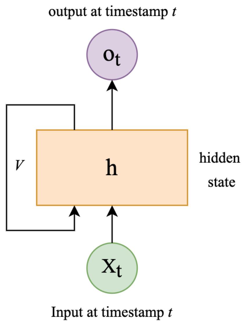
2.2. RNN
2.3. CNN & RNN Composites
3. Data Collection
3.1. Boma Locations
3.2. Sentinel-2 Data
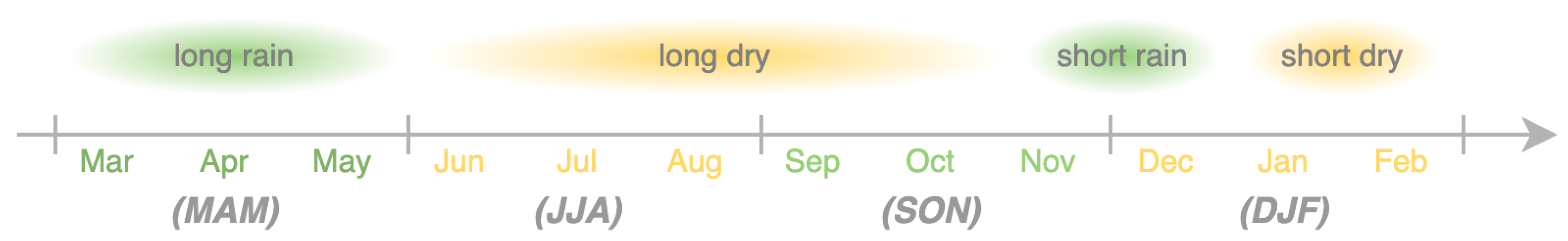
3.3. Season Alignment
4. Method
4.1. DCNN as Feature Extractor
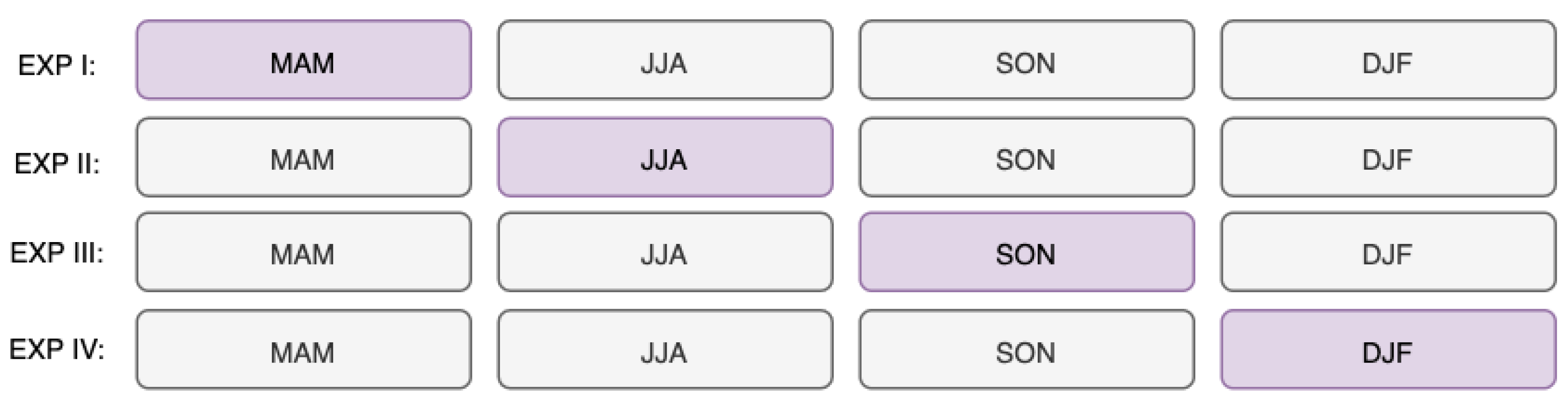
4.2. Cross-Season Validation
4.3. Deep Seasonal Network
5. Experiments
5.1. Cross-Season Validation
5.2. Performance of Deep Seasonal Network
5.3. Evaluating Robustness by Withholding a Season from Inference
5.4. Efficiency
6. Discussion
7. Conclusions
Author Contributions
Funding
Data Availability Statement
Conflicts of Interest
References
- Bank, A.D. A Critical Appraisal of the MDGs. MDGs in Tanzania: Progress and Challenges. 2009. Available online: https://sarpn.org/documents/d0001556/P1909-Afrodad_MDGs_Tanzania.pdf (accessed on 9 August 2023).
- Lawson, D.W.; Borgerhoff Mulder, M.; Ghiselli, M.E.; Ngadaya, E.; Ngowi, B.; Mfinanga, S.G.; Hartwig, K.; James, S. Ethnicity and child health in northern Tanzania: Maasai pastoralists are disadvantaged compared to neighbouring ethnic groups. PLoS ONE 2014, 9, 0110447. [Google Scholar] [CrossRef] [PubMed]
- Cheng, K.; Popescu, I.M.; Sheets, L.; Scott, G.J. Automatic Maasailand Boma Mapping with Deep Neural Networks. In Proceedings of the 2021 IEEE International Geoscience and Remote Sensing Symposium IGARSS, Brussels, Belgium, 11–16 July 2021; pp. 2839–2842. [Google Scholar] [CrossRef]
- Cai, H.; Zhu, L.; Han, S. ProxylessNAS: Direct Neural Architecture Search on Target Task and Hardware. arXiv 2018, arXiv:1812.00332. [Google Scholar]
- Cheng, K.; Popescu, I.; Sheets, L.; Scott, G.J. Analysis of Deep Learning Techniques for Maasai Boma Mapping in Tanzania. IEEE J. Sel. Top. Appl. Earth Obs. Remote Sens. 2022, 15, 3916–3924. [Google Scholar] [CrossRef]
- Cheng, K.; Bajkowski, T.M.; Scott, G.J. Evaluation of Sentinel-2 Data for Automatic Maasai Boma Mapping. In Proceedings of the 2021 IEEE Applied Imagery Pattern Recognition Workshop (AIPR), Washington, DC, USA, 12–14 October 2021; pp. 1–5. [Google Scholar] [CrossRef]
- Scott, G.J.; England, M.R.; Starms, W.A.; Marcum, R.A.; Davis, C.H. Training Deep Convolutional Neural Networks for Land-Cover Classification of High-Resolution Imagery. IEEE Geosci. Remote Sens. Lett. 2017, 14, 549–553. [Google Scholar] [CrossRef]
- Hu, F.; Xia, G.S.; Hu, J.; Zhang, L. Transferring Deep Convolutional Neural Networks for the Scene Classification of High-Resolution Remote Sensing Imagery. Remote Sens. 2015, 7, 14680–14707. [Google Scholar] [CrossRef]
- Chen, Z.; Zhang, T.; Ouyang, C. End-to-End Airplane Detection Using Transfer Learning in Remote Sensing Images. Remote Sens. 2018, 10, 139. [Google Scholar] [CrossRef]
- Fang, B.; Kou, R.; Pan, L.; Chen, P. Category-Sensitive Domain Adaptation for Land Cover Mapping in Aerial Scenes. Remote Sens. 2019, 11, 2631. [Google Scholar] [CrossRef]
- Panboonyuen, T.; Jitkajornwanich, K.; Lawawirojwong, S.; Srestasathiern, P.; Vateekul, P. Semantic Segmentation on Remotely Sensed Images Using an Enhanced Global Convolutional Network with Channel Attention and Domain Specific Transfer Learning. Remote Sens. 2019, 11, 83. [Google Scholar] [CrossRef]
- Qiu, C.; Mou, L.; Schmitt, M.; Zhu, X.X. Local climate zone-based urban land cover classification from multi-seasonal Sentinel-2 images with a recurrent residual network. ISPRS J. Photogramm. Remote Sens. 2019, 154, 151–162. [Google Scholar] [CrossRef]
- Chen, H.; Wu, C.; Du, B.; Zhang, L.; Wang, L. Change Detection in Multisource VHR Images via Deep Siamese Convolutional Multiple-Layers Recurrent Neural Network. IEEE Trans. Geosci. Remote Sens. 2020, 58, 2848–2864. [Google Scholar] [CrossRef]
- Scott, G.J.; Marcum, R.A.; Davis, C.H.; Nivin, T.W. Fusion of Deep Convolutional Neural Networks for Land Cover Classification of High-Resolution Imagery. IEEE Geosci. Remote Sens. Lett. 2017, 14, 1638–1642. [Google Scholar] [CrossRef]
- Scott, G.J.; Hagan, K.C.; Marcum, R.A.; Hurt, J.A.; Anderson, D.T.; Davis, C.H. Enhanced Fusion of Deep Neural Networks for Classification of Benchmark High-Resolution Image Data Sets. IEEE Geosci. Remote Sens. Lett. 2018, 15, 1451–1455. [Google Scholar] [CrossRef]
- Anderson, D.T.; Scott, G.J.; Islam, M.; Murray, B.; Marcum, R. Fuzzy Choquet Integration of Deep Convolutional Neural Networks for Remote Sensing. In Computational Intelligence for Pattern Recognition; Pedrycz, W., Chen, S.M., Eds.; Springer International Publishing: Cham, Switzerland, 2018; pp. 1–28. [Google Scholar] [CrossRef]
- Hurt, J.A.; Scott, G.J.; Davis, C.H. Comparison of Deep Learning Model Performance between Meta-Dataset Training Versus Deep Neural Ensembles. In Proceedings of the IGARSS 2019–2019 IEEE International Geoscience and Remote Sensing Symposium, Yokohama, Japan, 28 July–2 August 2019; pp. 1326–1329. [Google Scholar] [CrossRef]
- Bajkowski, T.M.; Scott, G.J.; Hurt, J.A.; Davis, C.H. Extending Deep Convolutional Neural Networks from 3-Color to Full Multispectral Remote Sensing Imagery. In Proceedings of the 2020 IEEE International Conference on Big Data (Big Data), Virtual, 10–13 December 2020; pp. 3895–3903. [Google Scholar] [CrossRef]
- Baghdasaryan, L.; Melikbekyan, R.; Dolmajain, A.; Hobbs, J. Deep Density Estimation Based on Multi-Spectral Remote Sensing Data for In-Field Crop Yield Forecasting. In Proceedings of the Proceedings of the IEEE/CVF Conference on Computer Vision and Pattern Recognition (CVPR) Workshops, New Orleans, LA, USA, 18–24 June 2022; pp. 2014–2023. [Google Scholar]
- Senecal, J.J.; Sheppard, J.W.; Shaw, J.A. Efficient Convolutional Neural Networks for Multi-Spectral Image Classification. In Proceedings of the 2019 International Joint Conference on Neural Networks (IJCNN), Budapest, Hungary, 14–19 July 2019; pp. 1–8. [Google Scholar] [CrossRef]
- Albertini, C.; Gioia, A.; Iacobellis, V.; Manfreda, S. Detection of Surface Water and Floods with Multispectral Satellites. Remote Sens. 2022, 14, 6005. [Google Scholar] [CrossRef]
- Chen, H.; Shi, Z. A Spatial-Temporal Attention-Based Method and a New Dataset for Remote Sensing Image Change Detection. Remote Sens. 2020, 12, 1662. [Google Scholar] [CrossRef]
- Gargees, R.S.; Scott, G.J. Deep Feature Clustering for Remote Sensing Imagery Land Cover Analysis. IEEE Geosci. Remote Sens. Lett. 2020, 17, 1386–1390. [Google Scholar] [CrossRef]
- Yang, A.; Hurt, J.A.; Veal, C.T.; Scott, G.J. Remote Sensing Object Localization with Deep Heterogeneous Superpixel Features. In Proceedings of the 2019 IEEE International Conference on Big Data (Big Data), Los Angeles, CA, USA, 9–12 December 2019; pp. 5453–5461. [Google Scholar] [CrossRef]
- Rashkovetsky, D.; Mauracher, F.; Langer, M.; Schmitt, M. Wildfire Detection From Multisensor Satellite Imagery Using Deep Semantic Segmentation. IEEE J. Sel. Top. Appl. Earth Obs. Remote Sens. 2021, 14, 7001–7016. [Google Scholar] [CrossRef]
- Wang, Y.; Li, Z.; Zeng, C.; Xia, G.S.; Shen, H. An Urban Water Extraction Method Combining Deep Learning and Google Earth Engine. IEEE J. Sel. Top. Appl. Earth Obs. Remote Sens. 2020, 13, 769–782. [Google Scholar] [CrossRef]
- Nejad, S.M.M.; Abbasi-Moghadam, D.; Sharifi, A.; Farmonov, N.; Amankulova, K.; Lászlź, M. Multispectral Crop Yield Prediction Using 3D-Convolutional Neural Networks and Attention Convolutional LSTM Approaches. IEEE J. Sel. Top. Appl. Earth Obs. Remote Sens. 2023, 16, 254–266. [Google Scholar] [CrossRef]
- Le, X.H.; Ho, H.V.; Lee, G.; Jung, S. Application of Long Short-Term Memory (LSTM) Neural Network for Flood Forecasting. Water 2019, 11, 1387. [Google Scholar] [CrossRef]
- Simonyan, K.; Zisserman, A. Very deep convolutional networks for large-scale image recognition. In Proceedings of the International Conference on Learning Representations, Banff, AB, Canada, 14–16 April 2014. [Google Scholar]
- He, K.; Zhang, X.; Ren, S.; Sun, J. Deep Residual Learning for Image Recognition. In Proceedings of the 2016 IEEE Conference on Computer Vision and Pattern Recognition (CVPR), Las Vegas, NV, USA, 27–30 June 2016; pp. 770–778. [Google Scholar] [CrossRef]
- Szegedy, C.; Liu, W.; Jia, Y.; Sermanet, P.; Reed, S.; Anguelov, D.; Erhan, D.; Vanhoucke, V.; Rabinovich, A. Going deeper with convolutions. In Proceedings of the Proceedings of the IEEE Conference on Computer Vision and Pattern Recognition, Boston, MA, USA, 7–12 June 2015; pp. 1–9. [Google Scholar]
- Huang, G.; Liu, Z.; Weinberger, K.Q.; van der Maaten, L. Densely connected convolutional networks. In Proceedings of the IEEE Conference on Computer Vision and Pattern Recognition, Honolulu, HI, USA, 21–26 July 2017; pp. 4700–4708. [Google Scholar]
- Tan, M.; Le, Q.V. EfficientNet: Rethinking Model Scaling for Convolutional Neural Networks. arXiv 2019, arXiv:1905.11946. [Google Scholar]
- Sundermeyer, M.; Ney, H.; Schlüter, R. From Feedforward to Recurrent LSTM Neural Networks for Language Modeling. IEEE/ACM Trans. Audio Speech Lang. Process. 2015, 23, 517–529. [Google Scholar] [CrossRef]
- Bahdanau, D.; Cho, K.; Bengio, Y. Neural Machine Translation by Jointly Learning to Align and Translate. arXiv 2014, arXiv:1409.0473. [Google Scholar]
- Graves, A.; Jaitly, N. Towards End-To-End Speech Recognition with Recurrent Neural Networks. In Proceedings of the 31st International Conference on Machine Learning, Bejing, China, 22–24 June 2014; PMLR Volume 32, pp. 1764–1772. [Google Scholar]
- Greff, K.; Srivastava, R.K.; Koutnik, J.; Steunebrink, B.R.; Schmidhuber, J. LSTM: A Search Space Odyssey. IEEE Trans. Neural Netw. Learn. Syst. 2017, 28, 2222–2232. [Google Scholar] [CrossRef] [PubMed]
- Xingjian, S.; Chen, Z.; Wang, H.; Yeung, D.Y.; Wong, W.k.; Woo, W.C. Convolutional LSTM Network: A Machine Learning Approach for Precipitation Nowcasting. arXiv 2015, arXiv:1506.04214. [Google Scholar]
- Hu, W.S.; Li, H.C.; Pan, L.; Li, W.; Tao, R.; Du, Q. Spatial–Spectral Feature Extraction via Deep ConvLSTM Neural Networks for Hyperspectral Image Classification. IEEE Trans. Geosci. Remote Sens. 2020, 58, 4237–4250. [Google Scholar] [CrossRef]
- Yin, J.; Qi, C.; Chen, Q.; Qu, J. Spatial-Spectral Network for Hyperspectral Image Classification: A 3-D CNN and Bi-LSTM Framework. Remote Sens. 2021, 13, 2353. [Google Scholar] [CrossRef]
- Zijlma, A. The Weather and Climate in Tanzania. 2020. Available online: https://www.tripsavvy.com/tanzania-weather-and-average-temperatures-4071465 (accessed on 9 August 2023).


| Architecture | Training Season | Precision | Recall | F1 |
|---|---|---|---|---|
| ResNet50 | MAM | 85.70% | 59.51% | 70.24% |
| JJA | 86.16% | 53.03% | 65.65% | |
| SON | 79.79% | 43.31% | 56.15% | |
| DJF | 75.48% | 24.45% | 36.94% | |
| ProxylessNAS | MAM | 65.25% | 47.28% | 54.83% |
| JJA | 70.07% | 44.78% | 54.64% | |
| SON | 63.19% | 28.79% | 39.55% | |
| DJF | 53.40% | 13.11% | 21.06% | |
| EfficientNet | MAM | 94.61% | 63.38% | 75.90% |
| JJA | 95.28% | 60.08% | 73.70% | |
| SON | 93.33% | 51.10 % | 66.04% | |
| DJF | 90.53% | 21.06 % | 34.17% |
| Train Data | Model | Precision | Recall | F1 | F1 Error Reduction |
|---|---|---|---|---|---|
| MAM | EfficientNet | 90.82% | 72.53% | 80.63% | – |
| DeepSN | 99.92% | 99.92% | 99.92% | 99.60% | |
| JJA | EfficientNet | 92.08% | 70.06% | 79.53% | – |
| DeepSN | 96.40% | 94.40% | 95.39% | 77.46% | |
| SON | EfficientNet | 89.51% | 63.32% | 74.17% | – |
| DeepSN | 90.69% | 83.19% | 86.78% | 48.82% | |
| DJF | EfficientNet | 90.10% | 40.64% | 55.95% | – |
| DeepSN | 78.46% | 57.09% | 66.09% | 23.02% |
| Architecture | Data Source | Precision | Recall | F1 |
|---|---|---|---|---|
| ProxylessNAS | VHR | 97.38% | 97.29% | 97.29% |
| ProxylessNAS | Sentinel-2 1C Annual Median | 73.15% | 73.90% | 73.42% |
| EfficientNet | Sentinel-2 1C Annual Median | 73.05% | 74.04% | 73.42% |
| DeepSN-ProxylessNAS | Sentinel-2 1C Multi-Temporal | 95.62% | 88.87% | 92.12% |
| DeepSN-EfficientNet | Sentinel-2 1C Multi-Temporal | 99.92% | 99.92% | 99.92% |
| EfficientNet (MAM-trained) | Sentinel-2 1C Multi-Temporal | 90.82% | 72.53% | 80.63% |
| Architecture | Scheme | Precision | Recall | F1 |
|---|---|---|---|---|
| EfficientNet-B0 | – | 86.64% | 63.38% | 73.20% |
| Deep Seasonal Net | 89.25% | 82.45% | 85.71% | |
| Deep Seasonal Net | 91.15% | 82.29% | 86.49% | |
| Deep Seasonal Net | 87.70% | 86.05% | 86.87% |
| Architecture | Data Source | Resolution | GPU | Time (h) |
|---|---|---|---|---|
| ResNet50 | VHR | 512 px | NVIDIA Tesla P100 | 8.57 |
| ProxylessNAS | VHR | 512 px | NVIDIA Tesla P100 | 6.92 |
| ResNet50 | Sentinel-2 1C | 64 px | NVIDIA GeForce RTX 3090 | 0.45 |
| ProxylessNAS | Sentinel-2 1C | 64 px | NVIDIA GeForce RTX 3090 | 0.49 |
| EfficientNet | Sentinel-2 1C | 64 px | NVIDIA Tesla T4 | 0.75 |
Disclaimer/Publisher’s Note: The statements, opinions and data contained in all publications are solely those of the individual author(s) and contributor(s) and not of MDPI and/or the editor(s). MDPI and/or the editor(s) disclaim responsibility for any injury to people or property resulting from any ideas, methods, instructions or products referred to in the content. |
© 2023 by the authors. Licensee MDPI, Basel, Switzerland. This article is an open access article distributed under the terms and conditions of the Creative Commons Attribution (CC BY) license (https://creativecommons.org/licenses/by/4.0/).
Share and Cite
Cheng, K.; Scott, G.J. Deep Seasonal Network for Remote Sensing Imagery Classification of Multi-Temporal Sentinel-2 Data. Remote Sens. 2023, 15, 4705. https://doi.org/10.3390/rs15194705
Cheng K, Scott GJ. Deep Seasonal Network for Remote Sensing Imagery Classification of Multi-Temporal Sentinel-2 Data. Remote Sensing. 2023; 15(19):4705. https://doi.org/10.3390/rs15194705
Chicago/Turabian StyleCheng, Keli, and Grant J. Scott. 2023. "Deep Seasonal Network for Remote Sensing Imagery Classification of Multi-Temporal Sentinel-2 Data" Remote Sensing 15, no. 19: 4705. https://doi.org/10.3390/rs15194705
APA StyleCheng, K., & Scott, G. J. (2023). Deep Seasonal Network for Remote Sensing Imagery Classification of Multi-Temporal Sentinel-2 Data. Remote Sensing, 15(19), 4705. https://doi.org/10.3390/rs15194705