Abstract
This paper proposes an information enhancement network based on self-supervised learning (SEL-Net) for runway area detection. During the self-supervised learning phase, the distinctive attributes of PolSAR multi-channel data are fully harnessed to enhance the generated pretrained model’s focus on airport runway areas. During the detection phase, this paper presents an improved U-Net detection network. Edge Feature Extraction Modules (EEM) are integrated into the encoder and skip connection sections, while Semantic Information Transmission Modules (STM) are embedded into the decoder section. Furthermore, improvements have been applied to the network’s upsampling and downsampling architectures. Experimental results demonstrate that the proposed SEL-Net effectively addresses the issues of high false alarms and runway integrity, achieving a superior detection performance.
1. Introduction
As essential military and civilian facilities, the detection of airport runway areas holds significant importance in emergency rescue, public services, and aircraft automatic landing [1]. Polarimetric Synthetic Aperture Radar (PolSAR) images exhibit such characteristics as all-day, all-weather capabilities, and they contain more abundant polarization information, which enables a more comprehensive reflection of object features. Consequently, the interpretation of PolSAR images holds high research value [2,3]. With the advancement of PolSAR technology, the acquisition of a vast amount of polarimetric synthetic aperture radar data has propelled the application of deep learning algorithms in PolSAR image interpretation research [4,5].
However, due to the lack of labeled images and the imaging mechanism that makes the boundary of the runway area blurred, the difficulty of image annotation is high. As a result, the current focus of airport runway area detection predominantly revolves around using optically acquired images that are easier to annotate and are available in larger quantities [6]. Due to the limited availability of annotated samples required for effective deep learning training, the detection of airport runway areas in PolSAR images mostly relies on traditional methods. Traditional polarized SAR image runway detection techniques involve manual feature extraction to identify regions of interest [7,8,9,10,11]. Subsequently, suspected targets are classified based on various manually set thresholds and using different classifiers, such as support vector machines [12,13,14,15], effectively filtering out false alarms from ground objects. Moreover, traditional methods necessitate the integration of prior information regarding airport runway areas, such as straight-line features, geometric characteristics, and dimensions of runways. However, the running time of these traditional methods is also long, and compared with some deep learning methods, it is difficult to guarantee the timeliness of detection [16].
With the development of deep learning theory, neural networks such as convolutional neural networks (CNN) [17,18,19,20] and quaternion neural networks (QNN) [21,22], have been well applied in PolSAR image processing. QNN is suitable for processing multidimensional and complex data, and can maintain the interdependence between channels. However, due to the large computational cost of QNN networks, and the lack of regularization methods and activation functions designed for QNN networks, the network layers are generally shallow when used, making it difficult to extract deeper features. Therefore, PolSAR image processing is still dominated by CNN. With the emergence of high-precision and generalizable semantic segmentation networks such as U-Net [17] and Deeplab V3 [20], CNN has been promoted for airport runway area detection. For instance, in reference [23], the integration of a geospatial context attention mechanism into the Deeplab V3 network enhanced the learning of geospatial features. Similarly, in reference [18], an innovative atrous convolution module was designed to expand the model’s receptive field, resulting in a reduced false alarm rate during airport runway area detection and yielding commendable detection outcomes.
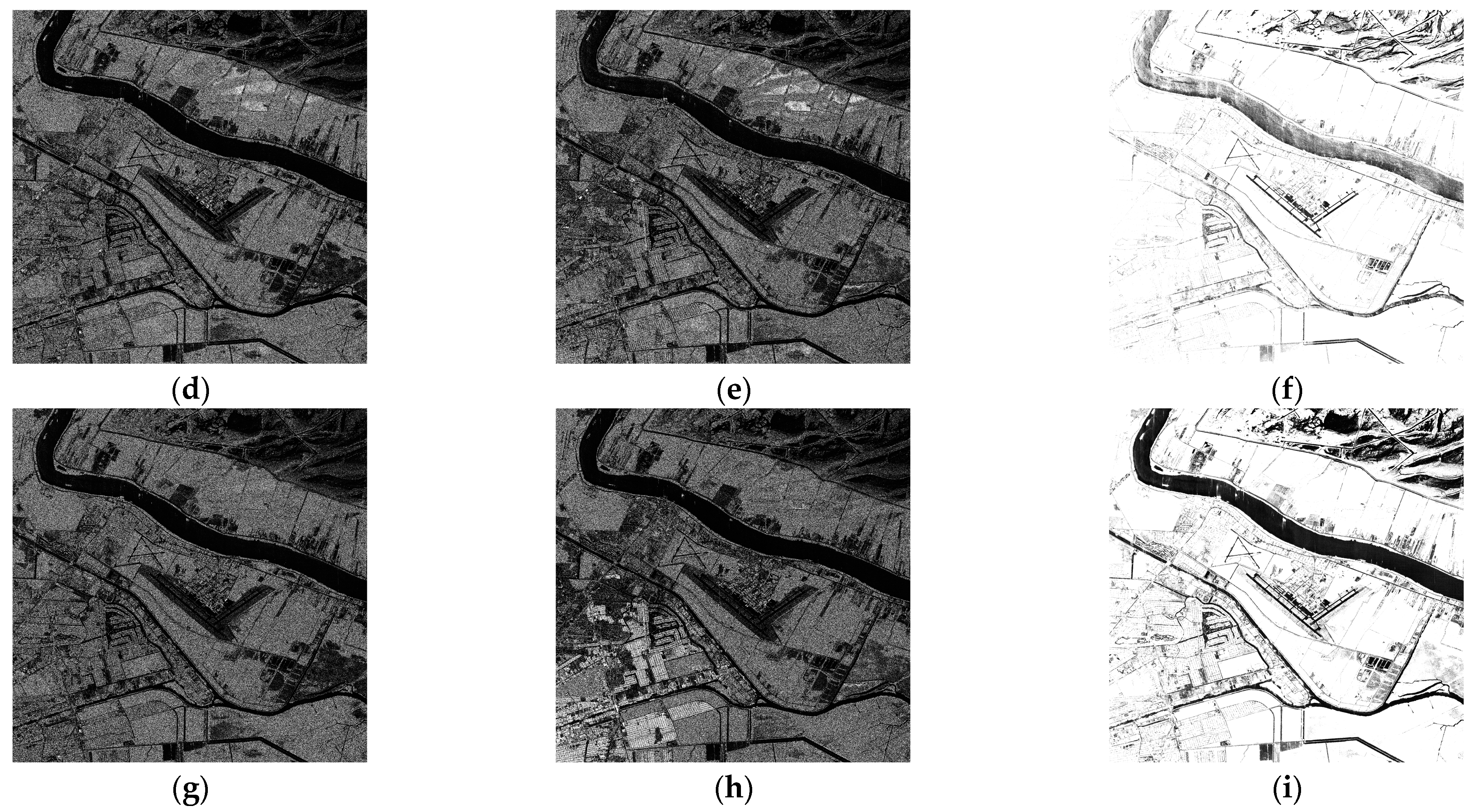
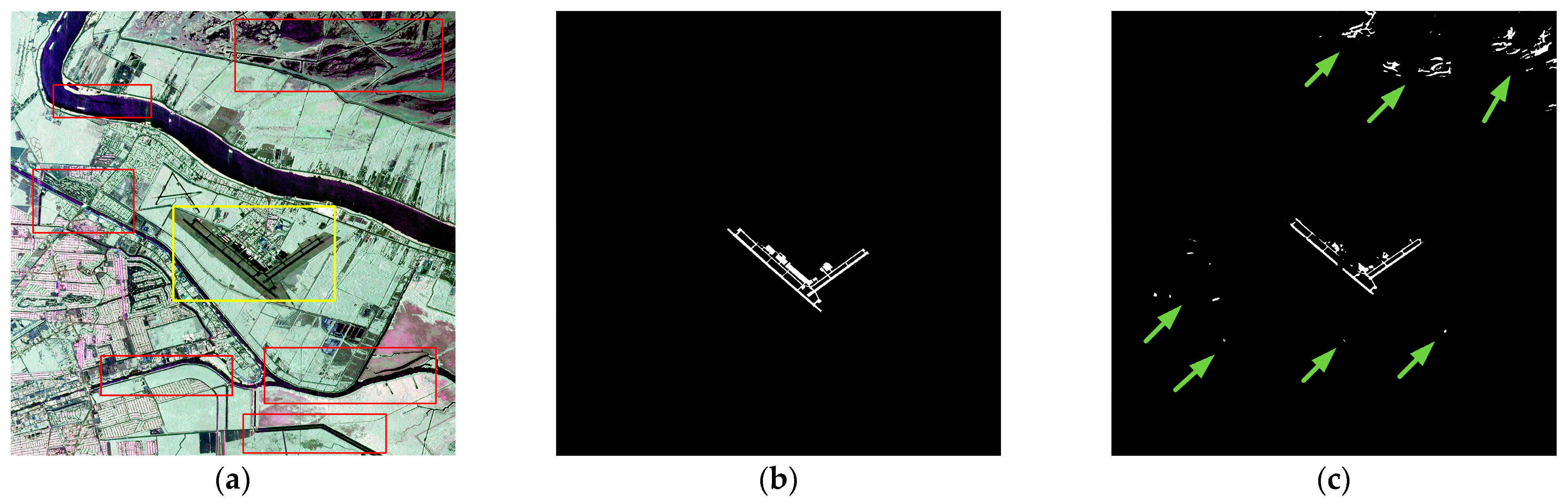
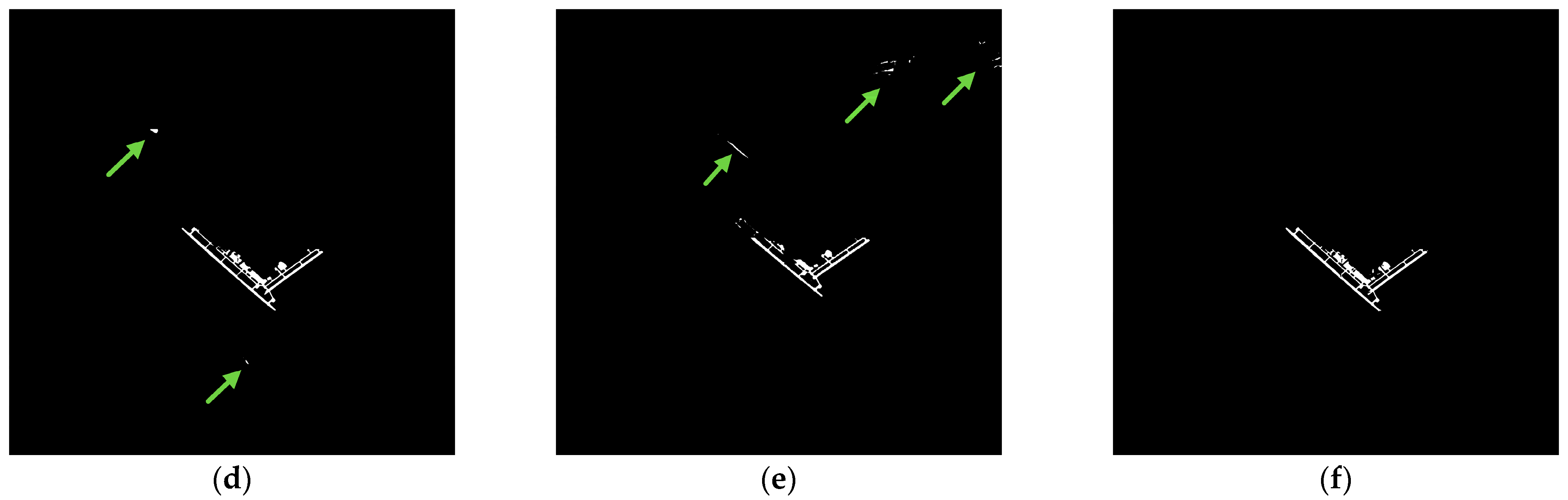
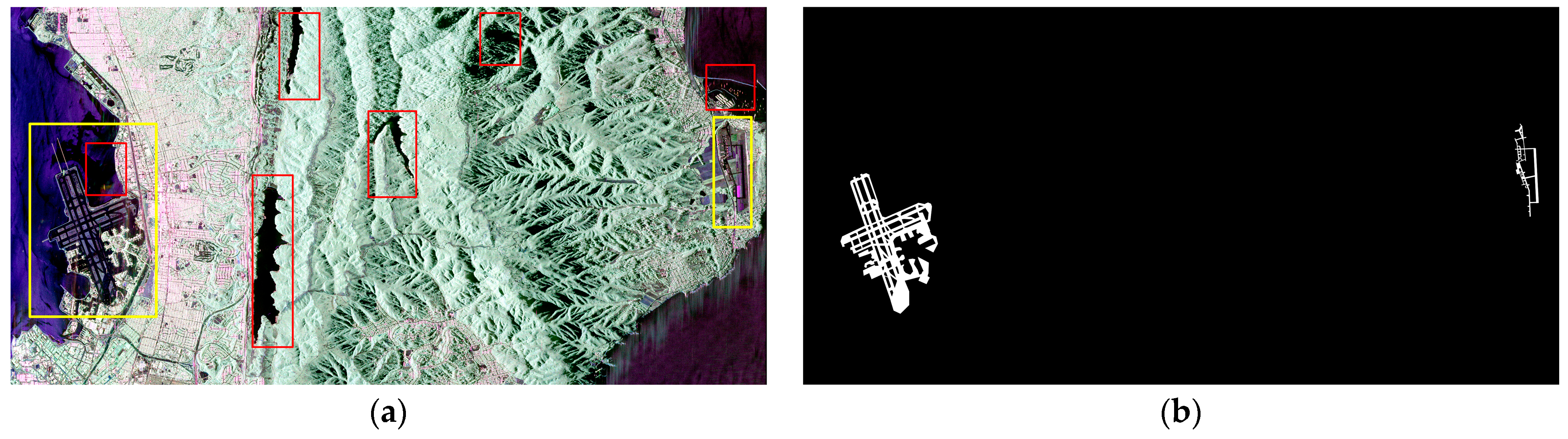
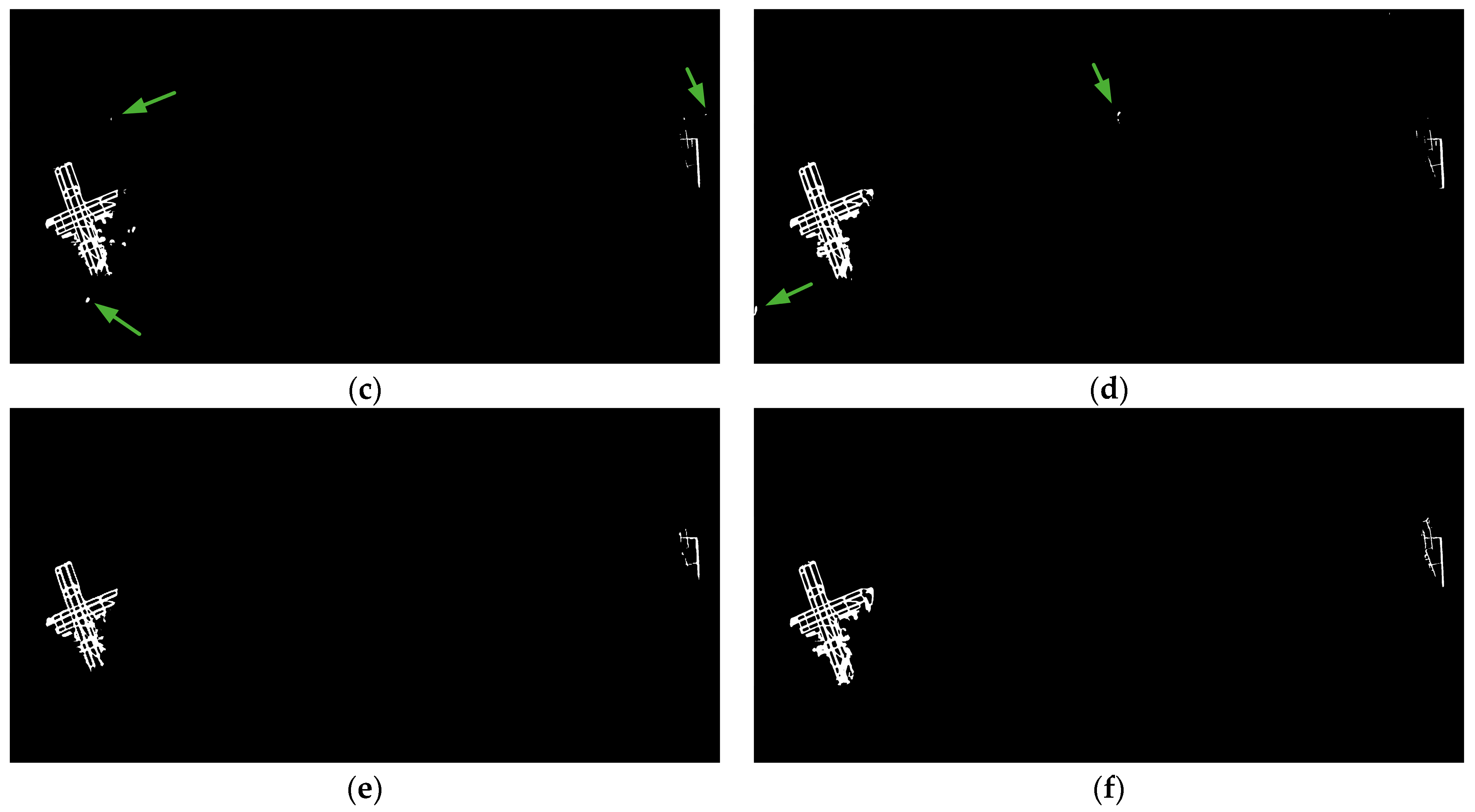
However, there are still shortcomings in some methods that use deep learning for airport runway area detection using PolSAR data [17,18,19,20,24]. Firstly, due to the imaging characteristics of PolSAR, ground targets such as rivers exhibit similar scattering properties to runways. This is manifested in the PauliRGB image, where colors appear quite alike, resulting in a significant number of false alarm occurrences. As depicted in Figure 1c, the detection results obtained from the notable Unet++ [19] network, an improved version of U-Net, are showcased. Unet++ has demonstrated favorable outcomes when applied to remote sensing imagery [25,26,27]. However, when utilized for runway area detection, certain limitations arise due to the scarcity of annotated training data. This data paucity impairs the network’s ability to extract deep semantic information specific to runway areas or results in the loss of critical semantic information during its propagation within the network. Consequently, the network struggles to effectively discern runways from other ground objects. Another shortcoming lies in the segmentation results, where the detection performance of certain runway or taxiway areas between runways is relatively poor. This is due to the presence of many narrow taxiways in the runway area of PolSAR images, which makes it difficult for the network to accurately detect. Adding edge information will enable the image to reference connected region information during detection. For example, as depicted in Figure 1f, the detection results obtained from the runway area segmentation algorithm D-Unet [18] illustrate its limitations in detecting taxiway regions within the red circle. Despite being an improved version of the U-Net network, specifically tailored for runway area detection, D-Unet still exhibits missed detections in taxiway regions. Indeed, numerous U-Net-based networks, with various improvements, have showcased remarkable performance across a multitude of image segmentation tasks [19,28,29,30,31]. However, when it comes to the specific challenge of runway area detection in PolSAR data, especially in large-scale scenarios, certain limitations hinder their overall effectiveness. These challenges are often rooted in the network’s structural designs, leading to the loss of critical semantic information during information propagation. For instance, the expression bottleneck structure mentioned in Inception V3 [32] could potentially result in information loss. Consequently, these factors significantly impact the network’s ability to achieve optimal runway area detection with PolSAR data. Of course, other PolSAR runway detection methods also have some shortcomings to a greater or lesser extent. Some common examples are: the detection scene is too small [33]; the detection time is too long; only the PauliRGB image is used without using other information from the matrix, which avoids the large amount of computation caused by complex numbers, but also loses a lot of useful information [18].
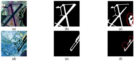
Figure 1.
Deficiencies of deep learning for runway area detection, The obvious false alarms and missed alarms are highlighted with red circles: (a) PauliRGB map of the Galveston Airport area; (b) Truth map; (c) Lack of deep semantic information; (d) PauliRGB map of the Kona Airport area; (e) Truth map; (f) Lack of edge information.
In recent years, there has been remarkable progress in the development of self-supervised learning algorithms. This approach has the distinct advantage of circumventing the resource-intensive data collection and annotation processes by leveraging auxiliary tasks to train models using the data itself [5]. The introduction of MOCO [34] has been a testament to the powerful capabilities of self-supervised learning. Models trained through self-supervised learning exhibit a robust ability to extract semantic information and demonstrate excellent generalization performance on downstream tasks, sometimes even outperforming supervised learning methods. Consequently, employing pre-trained networks obtained from self-supervised learning can effectively address the challenge of scarce annotated data in downstream tasks, enabling accurate extraction of deep semantic information. Although some research has applied self-supervised learning to PolSAR images and achieved outstanding results, the majority of these studies have focused on PolSAR image classification tasks [5,35]. However, these methods often involve dividing the images into homogeneous color blocks, which overlooks crucial information, like the shape of ground objects. As a result, these methods exhibit poor performance when directly applied to runway area detection tasks. The key challenge lies in integrating self-supervised learning with PolSAR images effectively, harnessing its advantages to precisely detect and segment airport runways despite limited annotated samples. Addressing this issue is crucial and forms the central focus and complexity of ongoing research efforts.
In response to the aforementioned challenges, this paper proposes a Self-Enhancing Learning Network (SEL-Net) for runway area detection, which incorporates self-supervised learning to enhance semantic and edge information. Firstly, building upon the self-supervised algorithm MOCO [34], SEL-Net utilizes the multi-channel nature of PolSAR data and introduces feature images that emphasize runway characteristics. By augmenting the number of positive samples and introducing pseudo-labeled images, the self-supervised network becomes more attentive to runway areas during pre-training. This allows the transferred pre-trained model to enhance its capability to extract deep features related to runways in the detection network. Furthermore, the segmentation network in SEL-Net includes a Semantic Information Transmission Module (STM) to facilitate the propagation of semantic information within the network, addressing the issue of information loss during transmission. Improvements are made to the up-sampling and down-sampling structures to further mitigate information loss. Additionally, to overcome insufficient edge information extraction, SEL-Net incorporates an Edge Information Extraction Module (EEM) and an Edge Information Fusion Module (EFM). These modules enhance the network’s ability to extract edge information.
The contributions of this paper can be summarized as follows:
- (1)
- A self-supervised learning-based PolSAR image runway area detection network, SEL-Net, is designed. By introducing self-supervised learning and improving the detection network, the effectiveness of runway area detection in PolSAR images has been significantly improved under conditions of insufficient annotated data, resulting in a reduction in both false positive and false negative rates.
- (2)
- By capitalizing on the distinctive traits of PolSAR data and employing the MOCO network, we obtain a pre-trained model that prioritizes the recognition of runway region features. Transferring this well-trained model to the downstream segmentation task effectively addresses the issue of insufficient deep semantic feature extraction from the runway region, which is previously constrained by the scarcity of PolSAR data annotations.
- (3)
- To enhance the U-Net network’s ability to extract edge information, we introduce EEM and EFM. Furthermore, we design a STM, and implement improvements to the up- and down-sampling processes to minimize the loss of semantic information during network propagation.
2. Related Work
2.1. Self-Supervised Learning
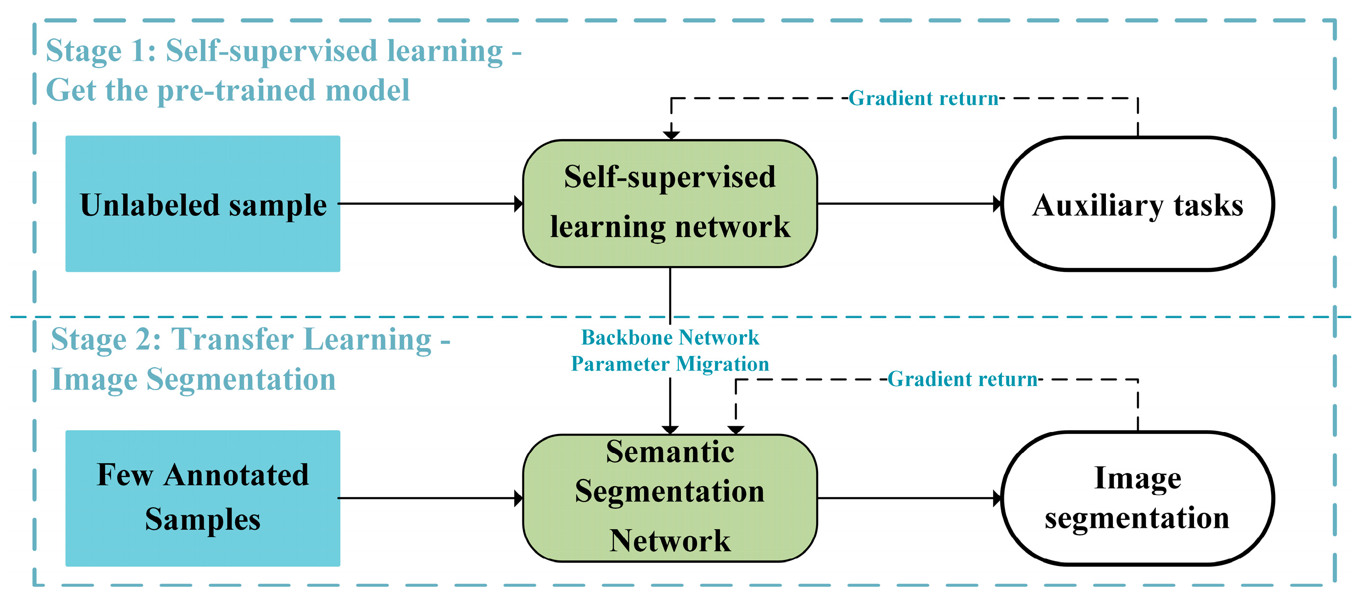
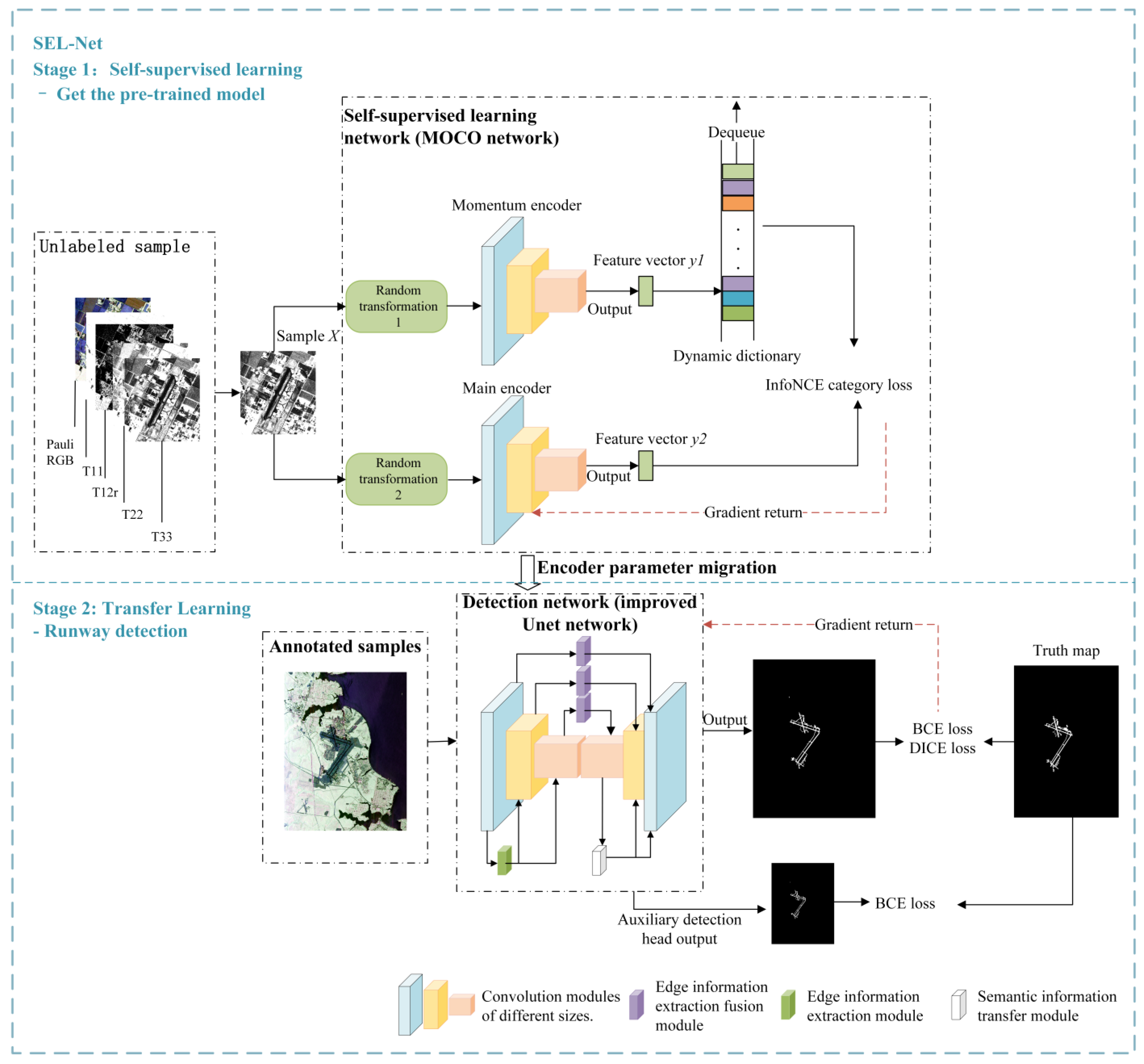
In recent years, self-supervised learning has achieved significant success [5]. This method does not require annotated data and yields pre-trained models with excellent generalization capabilities for downstream tasks. It aims to leverage the intrinsic representation of unlabeled data by designing auxiliary tasks as supervision, enabling the transfer of the pre-trained model to improve feature extraction in downstream tasks. The architecture for applying self-supervised learning to image segmentation tasks is depicted in Figure 2. The first stage involves self-supervised learning, where an unsupervised learning network is trained on unlabeled samples by completing predefined self-supervised auxiliary tasks. In the second stage, transfer learning occurs by migrating the backbone network parameters obtained from self-supervised learning to a semantic segmentation network, followed by training the network on a small number of labeled samples for segmentation tasks. Representative self-supervised learning networks include MOCO [34] and SimCLR [36]. They create positive sample pairs by using the same image and its transformed version and design auxiliary tasks to minimize the distance between the extracted features of positive sample pairs. In the field of image segmentation, self-supervised learning networks mostly adopt MOCO and similar networks, with the auxiliary task involving clustering of positive sample pairs and InfoNCE loss as the loss function. The downstream segmentation tasks often utilize widely used semantic segmentation networks, like U-Net [37]. Currently, self-supervised learning finds more applications in optical image tasks, where the pre-trained models improve the accuracy of detection, recognition, and segmentation tasks.
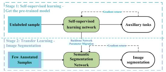
Figure 2.
Architecture of self-supervised learning for image segmentation tasks.
2.2. Semantic Segmentation Network
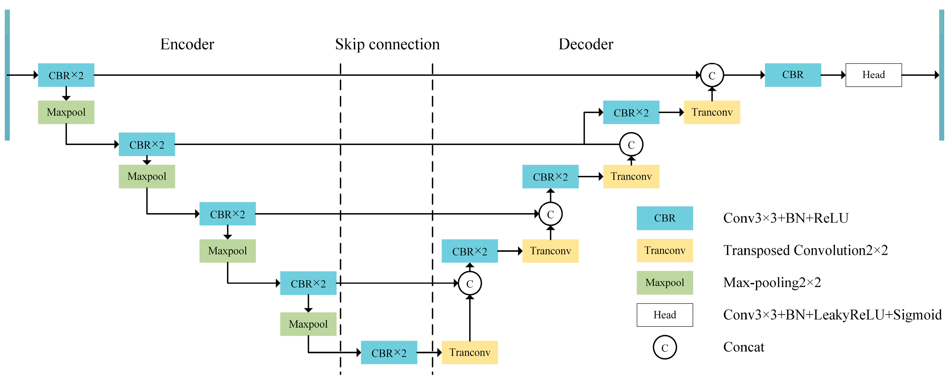
Semantic segmentation is a foundational computer vision task, and in recent years, numerous CNN-based segmentation networks have emerged. Broadly, these networks fall into two frameworks. The first, exemplified by the U-Net network [17] (as shown in Figure 3), consists of an encoder, decoder, and skip connections. The encoder employs convolutional operations to extract semantic information, while downsampling reduces computational parameters and mitigates background and noise interference. Skip connections provide shallow information, like color and texture, to the decoder. The decoder, in turn, upsamples deep semantic information and fuses it with the shallow information from skip connections to restore image details and dimensions. Finally, pixel classification is performed using a classification head. The second framework, represented by Deeplab V3 [20], focuses more on information fusion. Generally, in scenarios with limited annotated data, the U-Net architecture demonstrates distinct advantages.
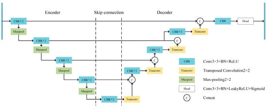
Figure 3.
U-Net network structure.
In recent years, numerous researchers have explored methods to enhance segmentation performance [28,30,38,39,40,41]. For instance, expanding the receptive field [28] or introducing feature fusion modules to extract multi-scale contextual information [20], similar approaches have been adopted in [18] to achieve notable results in runway area detection. Unet++ [19] proposed dense skip connections to fuse deep and shallow features, leading to impressive segmentation outcomes across diverse images. Incorporating edge information into the network to improve its edge processing capabilities is demonstrated in [41], and the recently proposed segmentation algorithm BA-Net [24] treats edge information extraction as a subtask to enhance the network’s capability to handle details. These innovative approaches have shown promising results in advancing segmentation effectiveness.
2.3. Representation of PolSAR Image Data
Unlike optical images that represent each pixel using three channels, PolSAR images typically use multiple channels to represent each pixel. The original PolSAR data is usually represented using matrices. These matrices can be decomposed using Pauli decomposition. Pauli decomposition has the property of keeping the total power constant. Therefore, the PauliRGB image, composed of the coefficients obtained from Pauli decomposition, can effectively reflect the polarization information of the matrices. Because the coherence matrix is easier to explain the physical meaning of the scattering process, and is easier to use for the design and analysis of the speckle filter, researchers usually use the coherence matrix to conduct research [42]. In 1970, Huynen proposed that the matrix can be decomposed into a sum of several independent components, and it can be represented as follows:
Among these, , , , , , , , and are Huynen parameters. These nine independent parameters contain certain scattering information [43] and can provide a more detailed reflection of the characteristics of different targets. Therefore, PolSAR images are usually described using matrices based on Huynen parameters. The specific meanings of the Huynen parameters are as follows:
- : Scattering power caused by the symmetry of the target;
- : Scattering power resulting from the overall asymmetry of the target;
- : Scattering power caused by the irregularity of the target;
- : Linear factor;
- : Measure of local curvature difference;
- : Local distortion of the object;
- : Overall distortion of the target;
- : Coupling between symmetric and asymmetric parts;
- : Directionality of the target.
3. Methodology
To address the issues in using deep learning for runway area detection, this paper proposes a self-supervised learning-based runway area detection network, named SEL-Net, which enhances semantic and edge information. The network architecture is shown in Figure 4. The training process is also divided into two stages: the first stage is self-supervised learning, where the unlabeled samples used for training are the PauliRGB images of each airport and the four feature channels forming four feature images, a total of five images, and the five images of each airport are treated as one category. The self-supervised learning network uses the MOCO [34] network, and the auxiliary task is extended to the airport classification task based on common image classification tasks. As a result, the pre-trained model obtained from self-supervised learning is more inclined towards extracting runway area features. The second stage is transfer learning, where the pre-trained network is transferred to the detection network for runway area detection tasks, and the training data consists of PauliRGB images and labeled images for runway area. The detection network used in this article is the improved U-Net. During detection, only the unlabeled PauliRGB image needs to be fed into the detection network, with the auxiliary detection head removed.
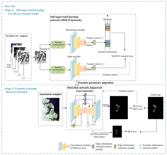
Figure 4.
General architecture diagram of the training network.
3.1. Self-Supervised Learning Network
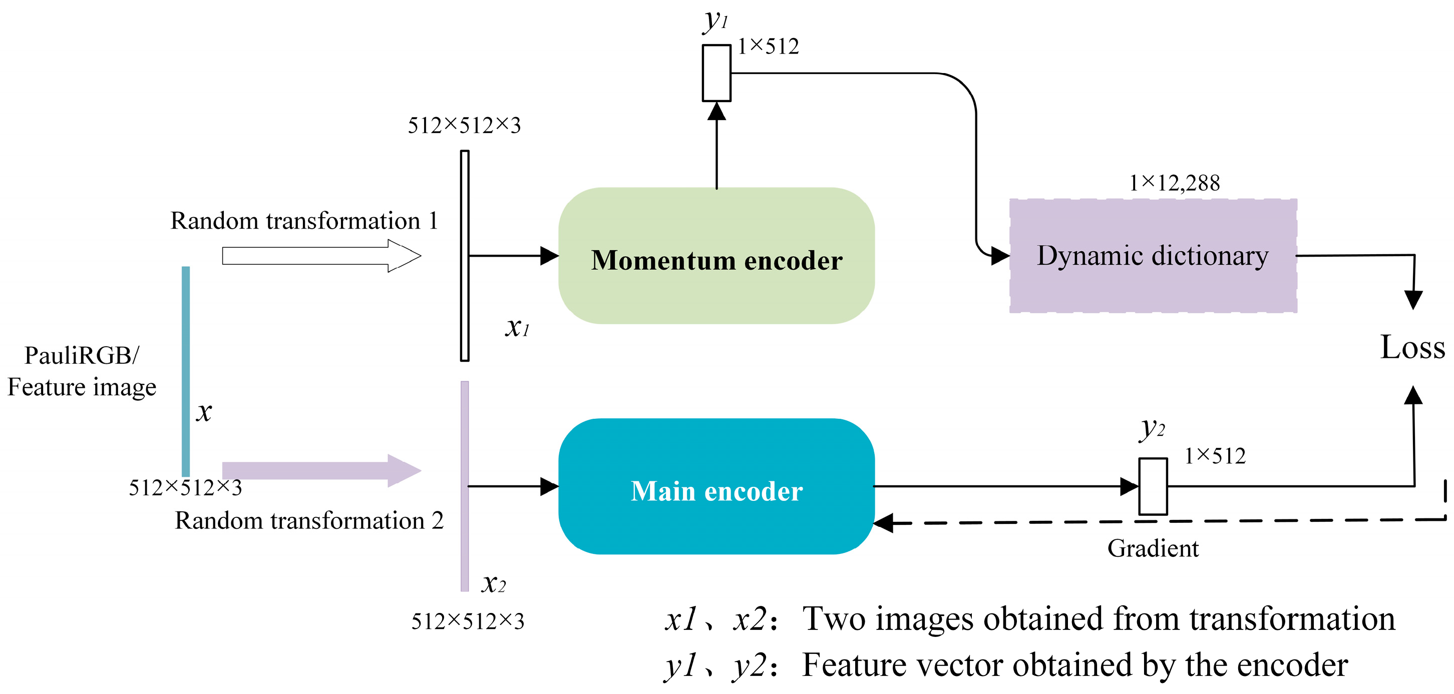
Based on the classic MOCO network in self-supervised learning, the network architecture is illustrated as shown in Figure 5. represents input PauliRGB images or feature images with airport identifiers. Currently, in the literature applying self-supervised learning to PolSAR data [5,35], the input samples for the self-supervised learning network consist of single PolSAR images. Building upon this, this paper introduces feature images with prominent runway area characteristics as additional input. In these feature images, the runway area stands out prominently while the remaining background information is relatively weak. These feature images approximate real annotated images and act as pseudo-labeled images, guiding the self-supervised learning network to focus more on extracting features from the runway area rather than the entire image context. After applying two different image transformations (such as cropping, color changes, etc.), we obtain two distinct images, and . After encoding the two images with an encoder, we obtain feature vectors and . Next, we place into a dynamic dictionary. We then calculate the contrastive loss between and all the feature vectors in the dynamic dictionary and backpropagate the gradients.
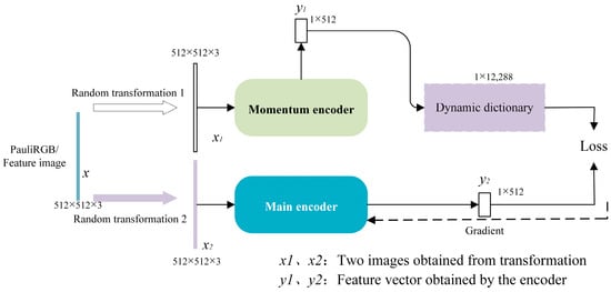
Figure 5.
Self-supervised learning network. (The data size of each step in the figure is based on the settings in our experiment as an example).
3.1.1. Encoder for MOCO
The main encoder and momentum encoder in the MOCO network adopt the structure shown in Figure 6, which is an improvement based on the encoder of the U-Net network. To reduce the loss, the ReLU activation function is replaced with LeakyReLU. To expand the receptive field, the first layer of 3 × 3 convolutions is replaced with a series of 7 × 1 convolutions, 1 × 7 convolutions, a batch normalization (BN) layer, and a LeakyReLU activation, forming an Starting Convolution Block (SC Block). Moreover, the strip convolution is used, which is advantageous for extracting features from strip-like objects, like runways. Finally, the last convolutional layer is changed to a classification head.
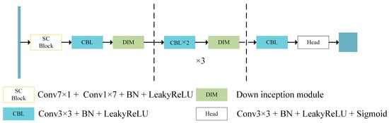
Figure 6.
Encoder structure in MOCO network.
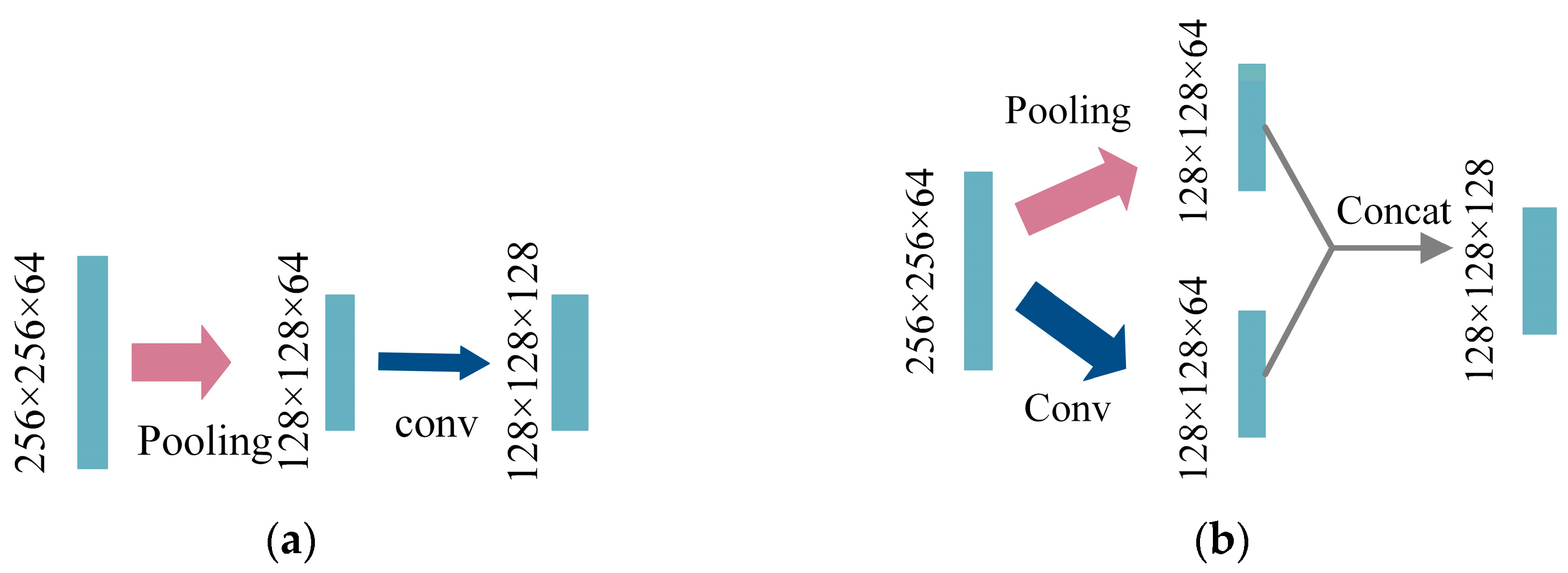
In the downsampling stage of the U-Net network’s encoder, the utilization of max-pooling operation introduces feature loss. Although downsampling with convolution can mitigate this issue, it comes at the cost of forsaking the advantages of max-pooling in reducing background interference and noise. Moreover, the Inception v3 paper [32] highlights the importance of avoiding representation bottlenecks within the model design. Representation bottleneck refers to the rapid compression of feature information during the process of transmission. To address this concern, we adopt the Inception V3’s proposed improvement approach by modifying the downsampling operation of the U-Net network to incorporate the Downsampling Inception Module (DIM). DIM replaces the conventional strategy of separate pooling and convolution with a simultaneous combination of convolution and pooling, followed by the concatenation of their results to prevent the formation of bottleneck structures. Upon observing the encoder structure of the U-Net network, we posit that the downsampling phase, where convolution is applied to augment the number of channels after each pooling layer, also engenders a representation bottleneck. Therefore, we apply the insights from Inception V3 to enhance the downsampling process in the U-Net network, yielding an improved DIM. The operational diagrams depicting the pre and post-improvement procedures are illustrated in Figure 7.
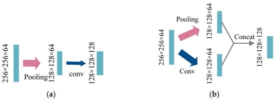
Figure 7.
Operational diagrams before and after the improvement of the bottleneck structure of the encoder stage: (a) The bottleneck structure of representation before improvement; (b) Improved downsampling module DIM. (Taking the second downsampling operation in the encoder stage as an example, 256 × 256 × 64 means that the size of the feature map is 256 × 256, and the number of channels is 64).
The term “conv” represents a 3 × 3 CBL (Convolution, Batch Normalization, and LeakyReLU) convolutional structure, and “pooling” refers to max-pooling with a stride of 2. The improved structure combines the advantages of both convolution and max-pooling downsampling.
The network structure of the dynamic encoder is the same as that of the main encoder. The only difference lies in the parameters updated after gradient backpropagation for the two encoders. At time step , the parameter update formula for the dynamic encoder is as follows:
where represents the parameters passed from the encoder, and represents the parameters of the dynamic encoder at the previous time step. This ensures that the features in the dynamic dictionary maintain consistency, even when they are generated by dynamic encoders with different parameters at different time steps.
3.1.2. Dynamic Dictionary
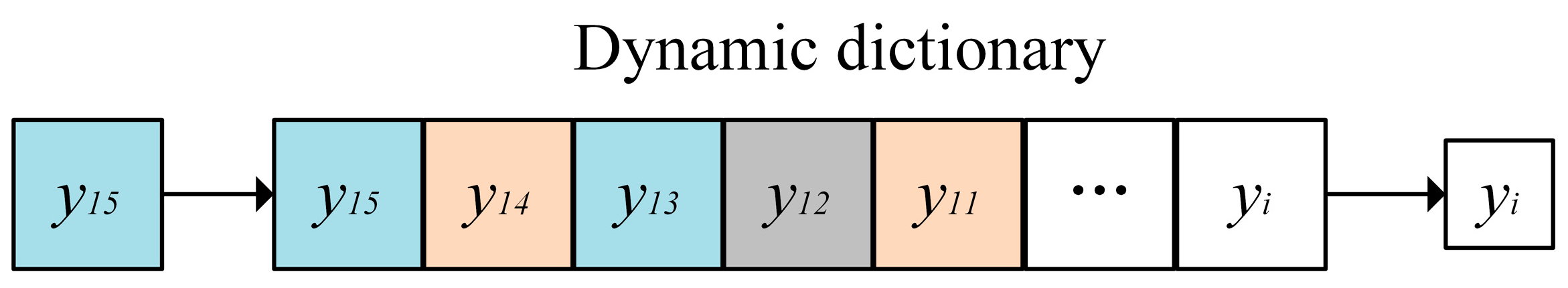
The self-supervised learning task of the MOCO network involves grouping an image with transformed images and into the same category. The introduction of feature images expands this self-supervised learning task into an airport classification task. It involves categorizing runway area images and their transformed counterparts belonging to the same airport into a single category. The goal is to determine the airport to which the queried runway area image belongs. During the loss calculation, the feature vectors obtained by encoding images from the same airport in the dynamic dictionary are treated as pairs of positive samples. The dynamic dictionary is shown in Figure 8.
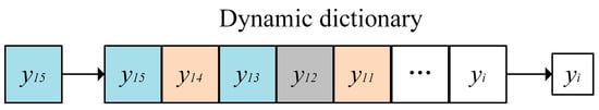
Figure 8.
Dynamic dictionary.
The dynamic dictionary maintains a fixed size, and when the vector length in the dictionary exceeds the dictionary size, the first-in first-out principle is adopted, and a feature will be taken out, as shown in Figure 8; after is put into the dynamic dictionary, because the length exceeds the preset size, the earliest feature that entered the dictionary is taken out. The MOCO network, in this context, focuses on comparing the similarity between two feature vectors, and , obtained from the transformations of a single image. Additionally, an airport class identifier constraint is introduced here. Consequently, all channel images and PauliRGB images derived from the same airport, along with their corresponding transformed images, are treated as positive sample pairs. In Figure 8, squares with the same color represent feature vectors obtained from the encoder for images belonging to the same airport. For instance, and , as well as and , correspond to feature vectors from the same airport. The objective is to minimize the loss function values for these pairs, ensuring that their similarity is maximized.
3.1.3. Loss Function
In Figure 5, all the features in the dynamic dictionary are compared with using a contrastive loss function. The objective is to maximize the similarity between feature vectors obtained from images belonging to the same airport (including feature images, PauliRGB images, and their transformed versions) and minimize the similarity between feature vectors from different airports. The loss function InfoNCE commonly used in contrastive learning is shown in Equation (3):
here, represents the number of feature encodings for negative samples in the dynamic dictionary. and are negative sample pairs, while and are positive sample pairs. is the cosine similarity calculation function, and is the temperature hyperparameter. After adding the constraint of the airport category, the loss function becomes:
here, represents the set of all images belonging to the same airport . The total loss is the sum of the losses for airports:
3.2. Detection Network
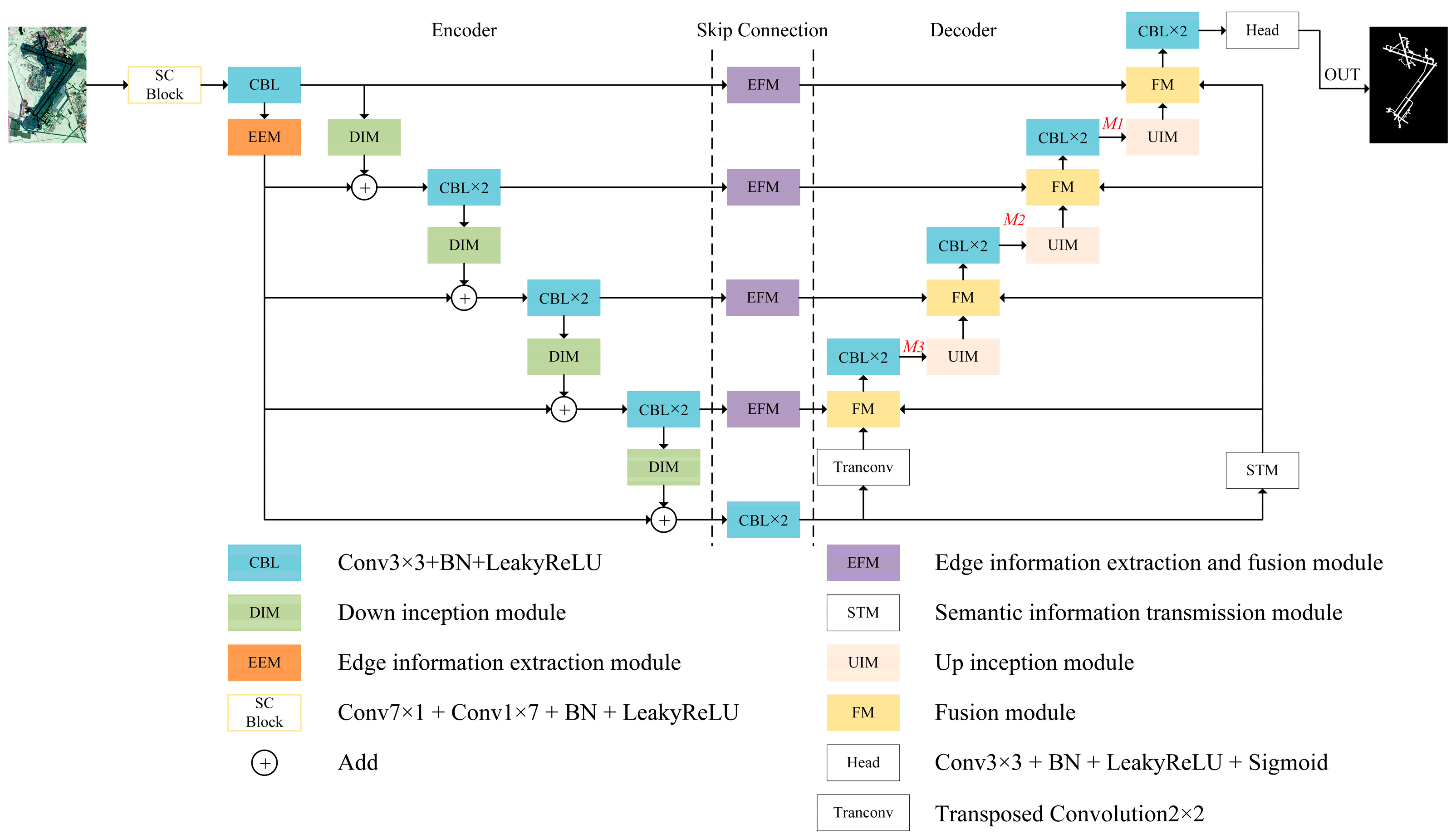
By analyzing the functions of different components within the U-Net network, this study proposes a redesign of its various parts. The Encoder is enhanced with the EEM, the skip connections incorporate the EFM, and the Decoder integrates the STM. Simultaneously, improvements are made to the downsampling operation of the Encoder and the upsampling operation of the Decoder. These modifications result in a detection network that is better suited for runway area detection tasks. The overall architectural diagram of the detection network is illustrated in Figure 9.

Figure 9.
Detection network.
3.2.1. Encoder
The role of the encoder in the U-Net network is to extract deep semantic information. However, during this process, edge information is generally extracted less effectively, and there is also a significant loss of information during the transmission in the encoder. To address these issues, an EEM is incorporated into the encoder to enhance edge information extraction. Additionally, the downsampling operation in the encoder is replaced with a DIM to improve the downsampling process. In addition, the convolutional kernel of the first convolutional layer of the encoder is changed from 3 × 3 to a concatenation of 7 × 1 and 1 × 7 to enlarge the receptive field of the model. The strip convolution is more favorable for extracting features of objects like runways with strip-like patterns.
Edge information extraction module (EEM). The EEM is introduced in this study, which incorporates shallow edge information with downsampled features from various layers. This integration enables the network to incorporate edge information during training at all levels, thereby enhancing the detection network’s ability to extract edge information during the encoder phase. The architecture of the EEM is illustrated in Figure 10.
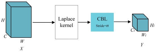
Figure 10.
Edge information extraction module.
The CBL module, illustrated in Figure 11, consists of a concatenation structure that includes a 3 × 3 convolution, batch normalization (BN), and a non-linear activation function. The stride of the convolutional operation is denoted by . Following the convolution, the size of the resulting edge feature map remains consistent with the dimensions of the downsampled feature map.
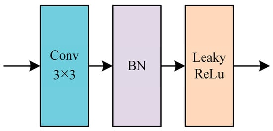
Figure 11.
CBL structure.
The edge information is derived from through a transformation, represented by the following formula:
here, L represents the Laplacian operator, which is defined by the following equation. denotes the convolution operation.
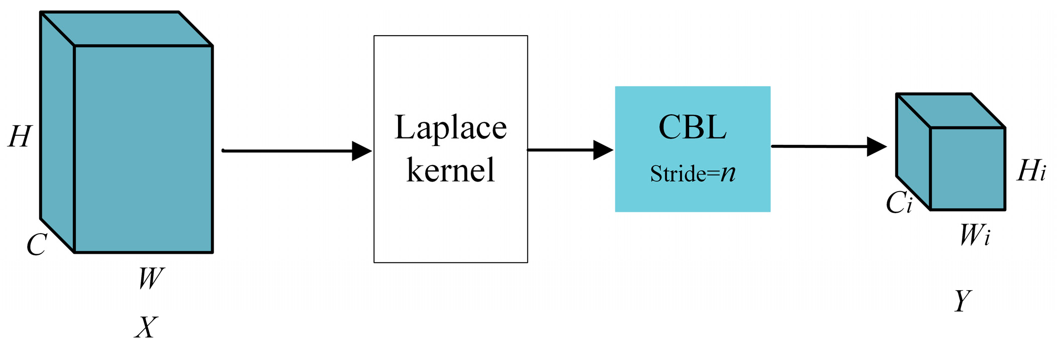
Downsampling Inception module (DIM). To reduce the loss caused by the bottleneck structure in the encoder of the U-Net, we replace the downsampling operation with the DIM mentioned in Section 3.1.1.
3.2.2. Skip Connection
The role of skip connections in the U-Net network is to transfer shallow features extracted from the encoder part to the decoder. These features are used in the decoder to reconstruct image details. Therefore, an EFM is incorporated during the skip connection phase to fuse edge information.
The EFM is used to further extract and fuse the edge information that is fed into the decoder. This enhances the decoder’s ability to extract and fuse edge information. The structure of the EFM is shown in Figure 12.
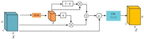
Figure 12.
Edge information extraction and fusion module.
Here, represents the sigmoid function, is a dimension channel concatenation term, and the formula for generating the edge fusion feature map is:
Here, represents the convolution operation, but with a kernel size of 1 × 1. First, the feature map undergoes processing through an EEM to generate the edge information map . Subsequently, the edge information weight is normalized to the range of (0,1) using the sigmoid function. When the edge information weight is relatively large, there is a risk of overshadowing other feature information, and the above formula helps to increase the importance of the feature map . On the other hand, when the edge information weight is relatively small, the same formula helps to reduce the significance of the feature map .
3.2.3. Decoder
The role of the U-Net network decoder is to fuse the deep semantic information extracted by the encoder with the shallow information transmitted through skip connections. It gradually upsamples the image size and performs pixel-wise classification through the final classification head. However, as the upsampling progresses, the deep semantic information gradually gets lost, and there are significant losses in information during the decoder’s propagation, leading to suboptimal segmentation results. To address this issue, a STM is introduced at the decoder end to facilitate the transmission of semantic information, and the upsampling operation is replaced with an Upsampling Inception Module (UIM).
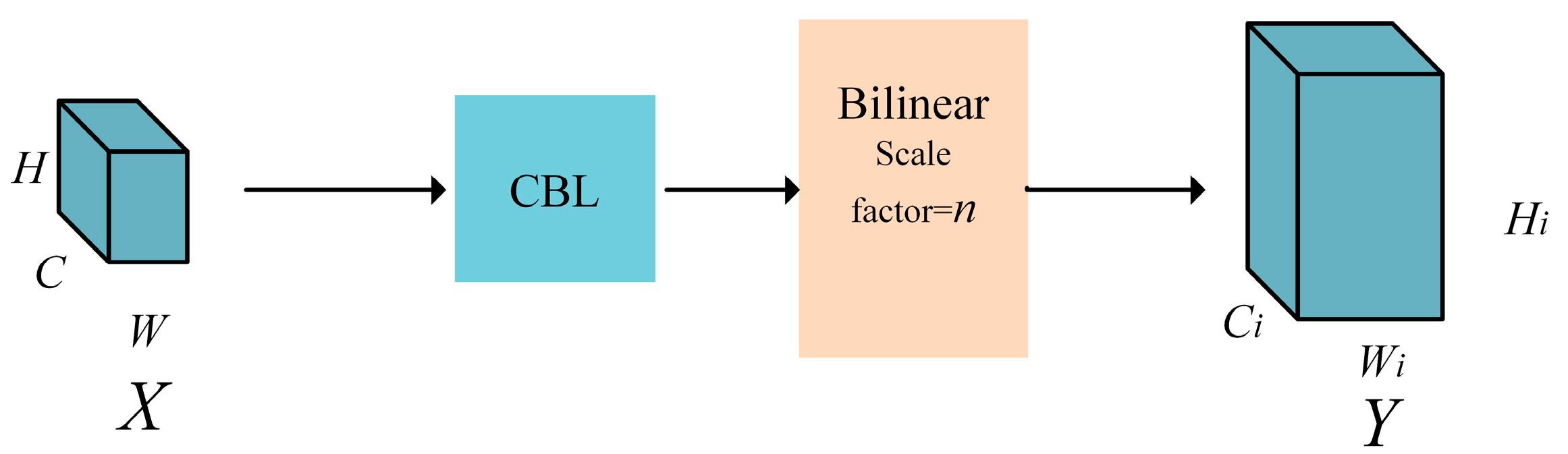
Semantic information transfer module (STM). In this paper, the STM is introduced to transfer deep semantic information from the neck to each stage after upsampling for feature fusion. The STM, as shown in Figure 13, begins by changing the channel number through convolution and then resizes the feature map using bilinear interpolation. This resizing ensures that the feature size after passing through the STM matches the feature size after upsampling. In the figure, “n” represents the parameter for the size expansion through bilinear interpolation.

Figure 13.
Semantic information transfer module.
The introduction of the STM enables the incorporation of deep semantic information at each step after upsampling, thereby addressing the issue of misclassification of categories during final detection caused by the loss of deep semantic information.
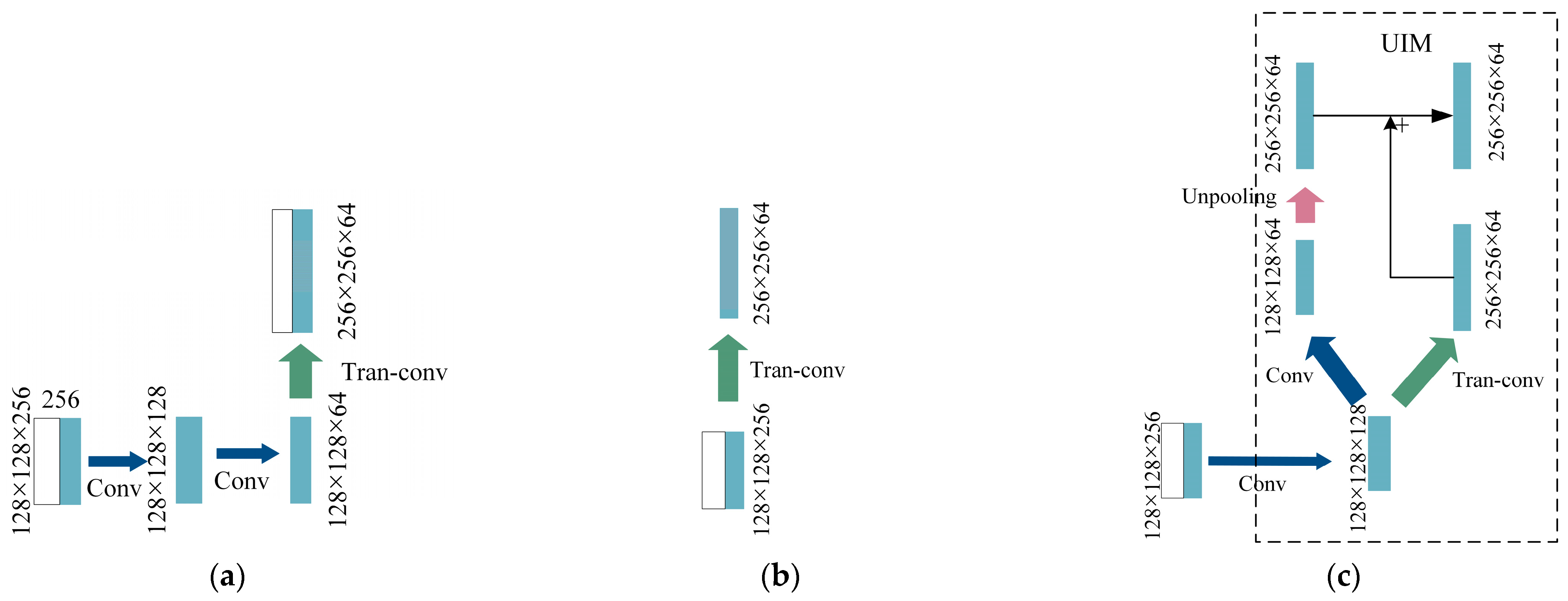
Upsampling Inception Module (UIM). In the decoder stage, performing two consecutive convolutions with halving of the channel number after fusing the information from skip connections can result in significant feature loss, as depicted in Figure 14a. The common practice is to skip these two convolutional operations and directly perform the upsampling operation, as shown in Figure 14b. However, this approach leads to a large computational burden and fuses numerous redundant feature maps, which has been found to yield suboptimal results in experiments. To address these challenges, a novel UIM is designed, inspired by the Inception V3 architecture, as illustrated in Figure 14c.
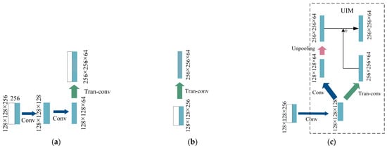
Figure 14.
Operation diagram before and after downsampling improvement: (a) The bottleneck structure of representation before improvement; (b) Usual practice; (c) Upsampling Inception module. (Take the third downsampling operation in the decoder stage as an example).
Here, Tran-conv represents a 2 × 2 transposed convolution upsampling, while Conv represents a 3 × 3 CBL convolution structure. Unpooling is performed by a stride of 2 in the form of deconvolution. The combination of these upsampling methods, which incorporate the characteristics of transposed convolution and deconvolution, can more effectively restore the information of the image and reduce the loss of semantic information during network propagation.
3.2.4. Feature Fusion Module (FM)
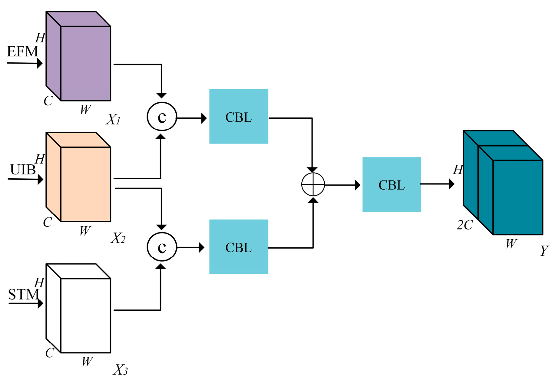
As shallow-level information is transmitted through skip connections, deep semantic information is propagated through STM, and information upsampling is performed, it is necessary to incorporate a fusion module FM to integrate the information, as illustrated in Figure 15.

Figure 15.
Feature Fusion Module.
Here, represents the feature map obtained through the EFM for skip connection propagation, represents the upsampled feature map, and represents the feature map after passing through the STM.
3.2.5. The Loss Function of the Detection Network
This study combines the commonly used BCE (Binary Cross-Entropy) loss and the DICE loss, which addresses the issue of sample imbalance. The network’s output is compared to the annotated images to calculate the loss. Furthermore, to supervise the edge features from EFM and the semantic information from STM, the , , and feature maps before the last three upsampling layers of the decoder in Figure 9 are passed through the detection head. The losses are then calculated against the annotated images using BCE loss. Therefore, the final loss of the detection network is:
where represents the Binary Cross-Entropy (BCE) loss from the network’s output, represents the Dice loss from the network’s output, and represents the BCE loss from the feature map. The others follow the same logic. represents the weight coefficient, and its design must satisfy the following equation:
Additionally, the weights for BCE loss and Dice loss are the same. Since is closer to the output, its weight needs to be larger than the weights of and feature maps but smaller than the weight of the output detection results. In this paper, the coefficients for to are taken as 0.3, 0.3, 0.2, 0.1, and 0.1, respectively.
4. Experiments and Analysis
4.1. Data Introduction
In the experiments, the data is derived from PolSAR images captured by the UAVSAR (Uninhabited Aerial Vehicle Synthetic Aperture Radar) system over the United States. The data corresponds to L-band fully polarized images. There are a total of 77 original images, each with a width of 3300 pixels and a length ranging from 6000 to 30,000 pixels. The distance resolution of the images is 7.2 m, and the azimuth resolution is 4.9 m. The dataset includes approximately 93 airports, out of which 31 airport runway areas are annotated manually. Apart from the airport regions, the image also covers various common land cover types such as ocean, rivers, urban buildings, farmland, mountains, forests, and others.
4.1.1. Introduction to the Self-Supervised Learning Phase Dataset
For the self-supervised learning segment, data is selected from 90 unlabeled airport areas and four common surrounding land types: ocean, farmland, mountain, and grassland. The data includes their respective PauliRGB images and feature maps, which have been cropped into images of size 512 × 512 pixels. In total, there are 470 such images in the dataset. By analyzing the visualization images of each channel in the matrix (as shown in Figure 16), and combining the physical information from Huynen’s parameters in Section 2.3, we identify four feature images with significant polarization characteristics in the airport runway region: , , , and (the real part of ). These feature images and the Pauli RGB image are combined as positive samples. In order to facilitate the use of the image transformation algorithm library and subsequent processing provided by the Pytorch framework, we expand each single-channel feature image by channel duplication to form a three-channel image.
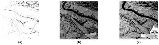
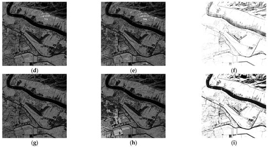
Figure 16.
Visualization diagram of each channel of T matrix: (a) channel; (b) channel; (c) channel; (d) channel; (e) channel; (f) channel; (g) channel; (h) channel; (i) channel.
4.1.2. Introduction to the Detection Phase Dataset
26 annotated PauliRGB images of airport runway areas will be processed using a sliding window with a stride of 50. The non-overlapping slices that do not contain the runway area will be removed, resulting in 380 annotated images with dimensions of 512 × 512 pixels. These images will be split into a training set and a validation set in an 8:2 ratio. The test dataset consists of five annotated PauliRGB images of airport runway areas with varying sizes. These images will be sliced using non-overlapping 512 × 512 windows, generating 98 images. During training, various online data augmentation techniques will be used to expand the dataset.
4.2. Experimental Parameter Settings
The experiment was conducted on the Pytorch 1.10 deep learning framework with two NVIDIA 3090 GPUs. Parameter settings: In the self-supervised learning phase, the batch size was set to 32, the dynamic dictionary size was 12,288, the initial learning rate was 0.1, the weight decay was 0.00001, the training cycle was 500, and the number of categories was set to 512. In the runway area detection phase, the batch size was set to 8, the initial learning rate was 0.0001, and the main trunk part during migration was frozen. The Adam optimizer was used for gradient descent. Both ablation experiments and comparative experiments were conducted using a fixed random seed number.
4.3. Evaluation Metrics
In order to quantitatively describe the experimental results, this study employed four commonly used accuracy metrics to evaluate the performance of the network. These metrics are Pixel Accuracy (PA), Recall, F1 Score (F1), and Mean Intersection Over Union (MIoU) [18]. These metrics were chosen to assess the detection performance of the network comprehensively. The network complexity is measured by model parameter size (Params), floating-point operations per second (FLOPs), and frames per second (FPS).
4.4. Experimental Results and Analysis
4.4.1. Selection of Data Transformations for Part of Self-Supervised Learning
Due to the significant differences between PolSAR (Polarimetric Synthetic Aperture Radar) images and optical images, the data transformations commonly used in most self-supervised learning networks for optical images might not be suitable for PolSAR images. In fact, using inappropriate transformation methods can negatively impact the performance of the pre-trained models generated through self-supervised learning [36]. To address this issue, eight common image transformation methods were selected: image displacement, color enhancement, random erasing, image flipping, image rotation, cropping, Gaussian smoothing, and adding noise. These transformations were combined in pairs, and the models were trained for 300 epochs. The resulting pre-trained models were then transferred to the U-Net network for the runway area detection task. The pre-trained model parameters were frozen, and fine-tuning training was conducted for 100 epochs, with the baseline being the MIoU of 39.59% without the pre-trained model. The experimental results are shown in Figure 17.
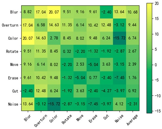
Figure 17.
Ablation experiment results of data transformation.
From the figure, it can be observed that random noise, random erasing, and displacement transformations can all lead to significant negative optimization effects on the network, while Gaussian smoothing, on the contrary, performs the best. Through the analysis in this paper, it is believed that this is because the feature maps are weakened for smaller interfering objects after Gaussian smoothing, thereby highlighting the features of larger runway area targets. Therefore, color enhancement, image flipping, image rotation, cropping, and Gaussian smoothing are chosen as the five image transformation methods in the self-supervised learning network.
4.4.2. Experiments for Self-Supervised Learning
To verify the effectiveness of the self-supervised learning part of the network, this study compares representative CNN-based self-supervised learning methods, MOCO [34], and SimCLR [36], which utilize positive and negative sample contrast. Firstly, the dataset is fed into these three networks, and they are trained for 500 epochs, with the classification number set to 512 and the dynamic dictionary size set to 12,288. Additionally, the dataset with the feature images removed is also fed into our proposed method to verify the effect of adding feature images. The obtained pre-trained models are then transferred to the U-Net network for frozen pre-trained model parameter airport runway area detection experiments. The experimental results are shown in Table 1.

Table 1.
Comparative experiments in the self-supervised learning part.
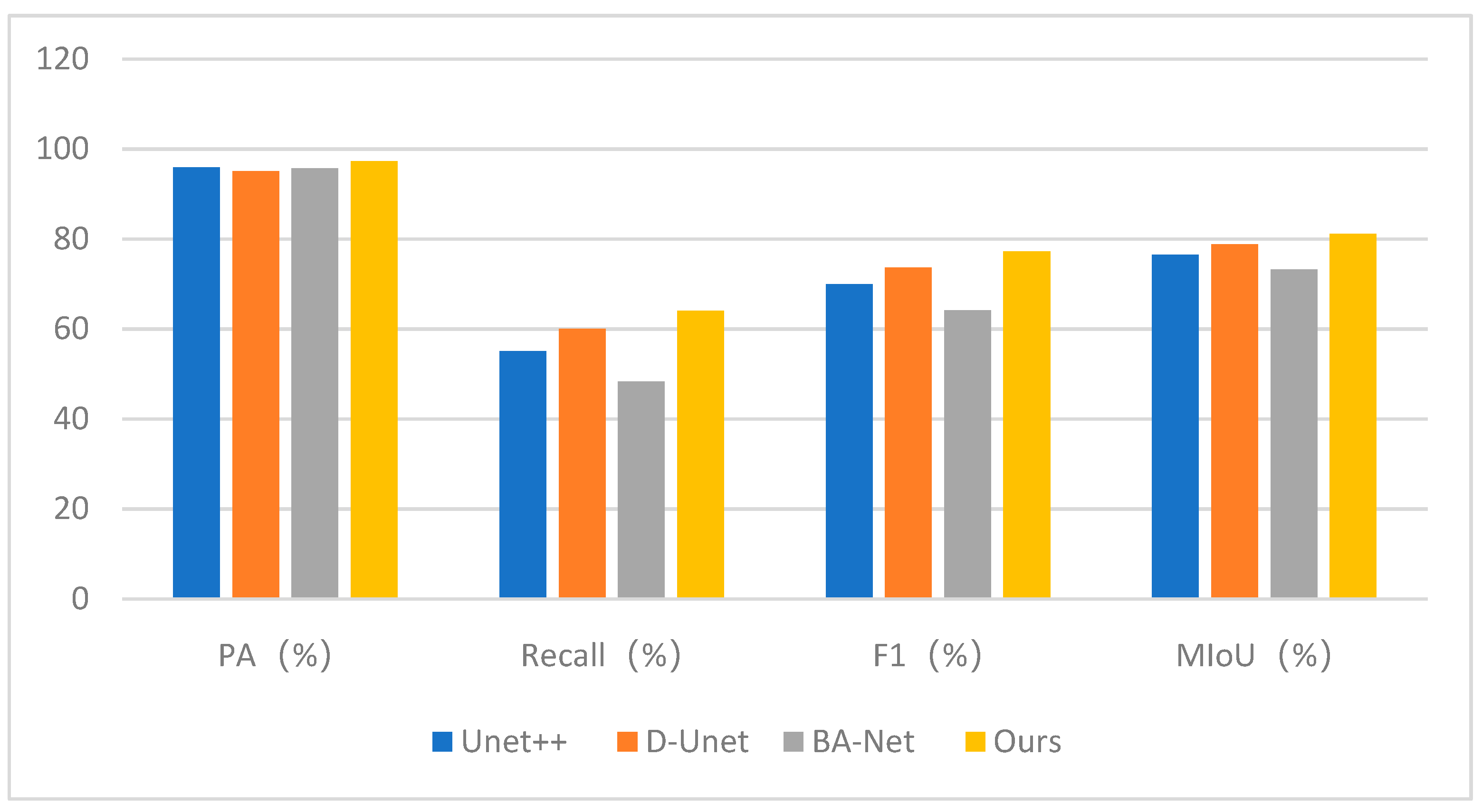
It can be observed that the pre-trained learning models obtained using the method proposed in this paper achieve an MIoU of 62.12% on downstream tasks, which is significantly higher than the results of the other two self-supervised learning methods. Furthermore, it can be seen from Figure 18 that the other three evaluation metrics also outperform the other two self-supervised learning methods. However, when the feature images are removed, the proposed method essentially degrades into the MOCO network for image classification. Due to the limited number of images, the performance is actually poor.
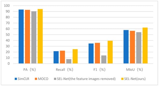
Figure 18.
The bar chart of the comparison experiment results of the self-supervised part.
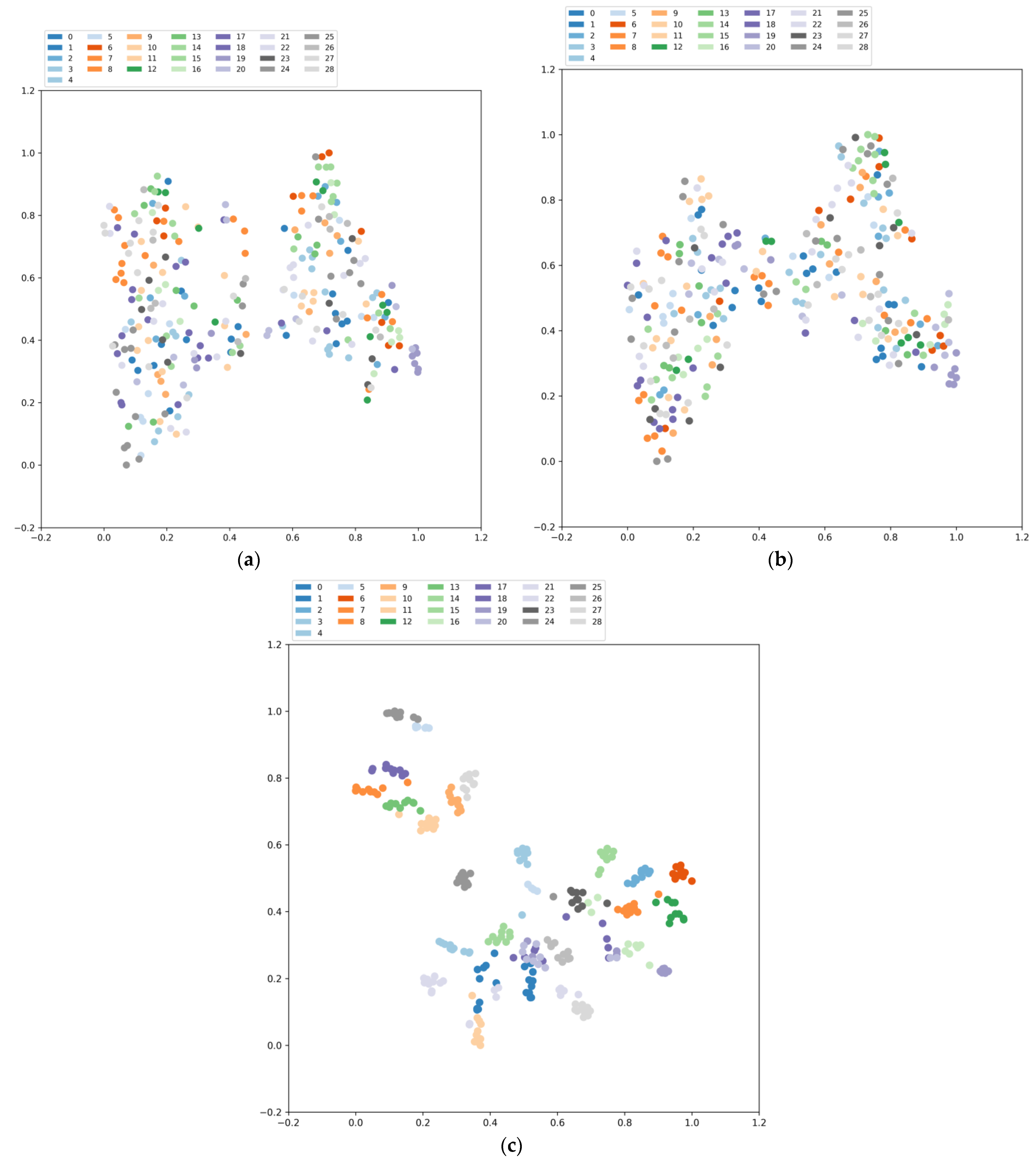
Then, 25 images of airports and four types of terrain slices (ocean, farmland, mountains, grassland) are randomly selected. These images, along with their PauliRGB images and the selected four feature images and their 90-degree rotated images, a total of 290 images, are fed into the pre-trained models obtained from our proposed method, MOCO, and SimCLR. The results are then subjected to dimensionality reduction using t-SNE, where dots of the same color represent images from the same airport or terrain slice. The results are shown in Figure 19. It can be observed that our proposed method, by extending the self-supervised learning task to classify images into airport categories, focuses more on runways. The dimensionally reduced features are more concentrated between different classes. On the other hand, the other two methods, without the constraint of including the airport category, show more scattered results. This experiment demonstrates the effectiveness of our proposed method.
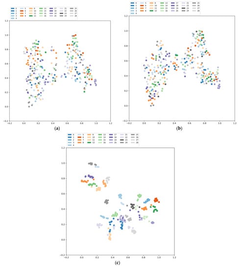
Figure 19.
t-SNE dimensionality reduction visualization: (a) MOCO; (b) SimCLR; (c) Ours.
Finally, the Grad-CAM technique was employed to visualize the parameter responses of the last convolutional layer, providing insights into the areas of interest in the model. One randomly selected PauliRGB image of the airport was visualized, and the results are depicted in Figure 20. It can be observed that our proposed method, due to extending the self-supervised learning task to classify the images into their respective airport categories, focuses more on the runways, while the other two methods tend to emphasize the global features of the images. As a result, transferring the pre-trained model obtained from the self-supervised learning part of our proposed method to the encoder of the downstream detection network and fine-tuning it enables the encoder to extract features more related to the airport runway areas, effectively addressing the issue of insufficient extraction of deep semantic information caused by the scarcity of annotated images.
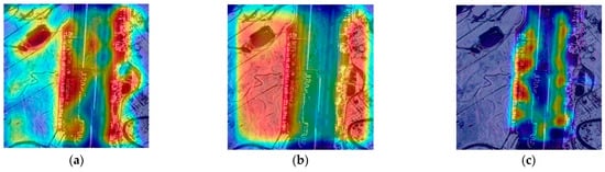
Figure 20.
Grad-CAM heat map visualization: (a) MOCO; (b) SimCLR; (c) Ours.
4.4.3. Ablation Experiment of SEL-Net
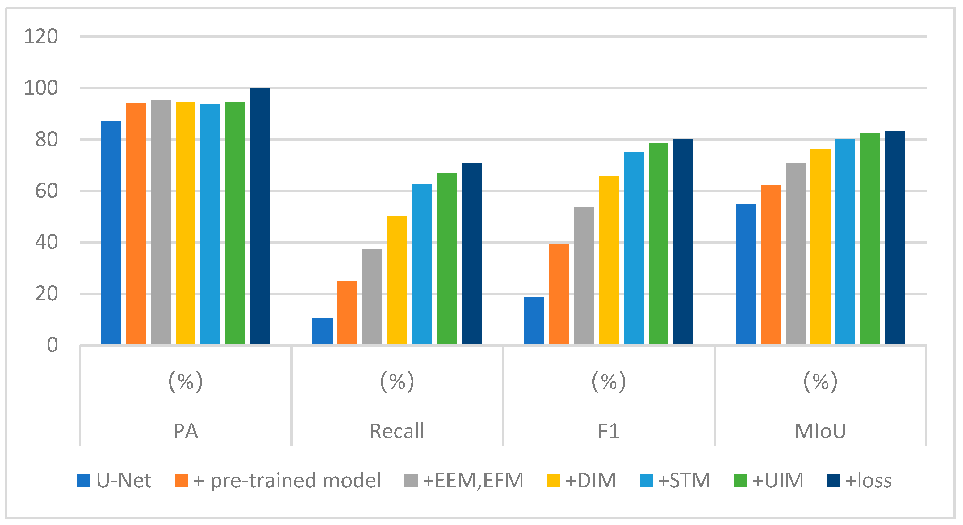
To evaluate the effectiveness of the proposed network in improving the U-Net network by incorporating pre-trained models, edge information enhancement modules, semantic information transfer modules, upsampling, and loss functions, an ablation study was conducted based on the U-Net network. All ablation experiments were designed with identical hyperparameters. The experimental results are shown in Table 2. The bar chart of the experimental results is shown in Figure 21.
Table 2.
Main ablation experiments for SEL-Net.

Figure 21.
Bar chart of the main ablation experiment results.
The change in network accuracy after adding each module in turn can be seen from the table, and it can also be seen from Figure 21 that the indicators show an upward trend after adding the modules in turn, indicating the effectiveness of each module; especially, the addition of edge information makes the accuracy show a significant improvement. Taking the detection results at Panama Pacific International Airport as an example, the impact of each module on the improvement of the results is observed. The image size is 2000 × 2000, and this airport has a relatively small size with multiple and shorter taxiways, which better reflects the model’s ability to handle semantics and edges. The runway area in the detection result is enlarged, as shown in Figure 22. In Figure 22d, the inclusion of the pre-trained model enhances the capability to extract deep semantic information, resulting in the detection of the apron area on the upper left part of the runway area indicated by the arrow, significantly reducing the miss detection rate. It can be observed from Figure 22e that the addition of edge information makes the contour of the runway area more prominent, and the main runway part can be detected more completely. The taxiways on both sides of the main runway also become more apparent. As seen in Figure 22f, the improved downsampling makes the airport’s lines connect more continuously, and the apron area indicated by the arrow is detected. Figure 22g shows that the inclusion of the semantic transfer module allows for the detection of the apron and stand areas indicated by the arrow. The improved upsampling makes the apron area at the arrow in Figure 22h more complete.
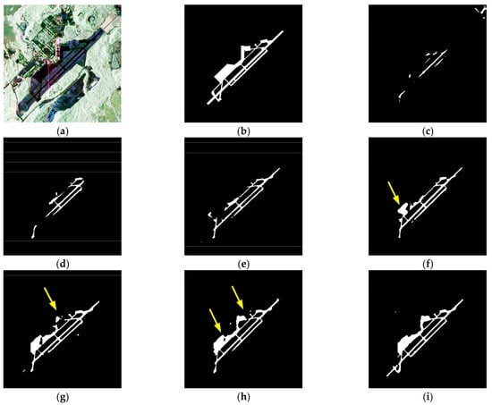
Figure 22.
Enlarged images of the airport area in some ablation experiment detection results, using Panama Pacific International Airport as an example. The area indicated by the arrow has seen a significant increase in detection results after the addition of modules: (a) PauliRGB image; (b) Ground truth image; (c) U-Net network; (d) Add pre-trained model (without DIM); (e) Add EEM, EFM; (f) Add DIM; (g) Add STM; (h) Add UIM; (i) Add loss.
In order to further verify whether the improvements in the modules enhance edge information, semantic information, and reduce loss during network feature extraction, this paper visualizes the feature maps in the feature extraction process of the Panama Pacific International Airport. The image size is 512 × 512 pixels, and PauliRGB is shown in Figure 23a. The visualization includes the last down-sampled feature map of the encoder without any modules added (Figure 23b) and the last up-sampled feature map of the decoder (Figure 23c). Finally, all four parts mentioned above are sequentially stacked and integrated into the network.
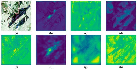
Figure 23.
The resulting image of the feature map visualization, taking Panama Pacific International Airport as an example: (a) PauliRGB image; (b) Visualization before the last downsampling without adding any modules; (c) Visualization of the last upsampling without adding modules; (d) Visualization before the last downsampling after adding EEM and EFM; (e) Visualization of the last upsampling after adding EEM and EFM; (f) Visualization before the last downsampling after improving the downsampling structure; (g) Visualization of the last upsampling after adding STM; (h) Visualization of the last upsampling after improving the upsampling structure.
- Visualize the channels of the last down-sampled layer before and after the incorporation of edge information, as well as the channels of the last up-sampled layer, as shown in Figure 21d,e. It can be observed that the addition of the EEM aids in extracting edge information during the down-sampling stage and the skip-connection stage, making the outlines of the runway area more distinct.
- Visualize the channel map before the last down-sampling of the improved down-sampling structure, as shown in Figure 21f. The increased brightness in the image represents that the down-sampling has retained more semantic information of the image while also reducing the information of non-runway area objects.
- Visualize the channel map after the last up-sampling of the improved up-sampling structure, as shown in Figure 21g. It can be observed that the addition of the STM has made the runway lines clear and continuous.
- Visualize the channel map after the last up-sampling of the improved up-sampling structure, as shown in Figure 21h. It can be observed that the network with the improved up-sampling structure has reduced the loss in feature map processing, resulting in clearer runway lines.
4.4.4. Comparative Experiment with SEL-Net
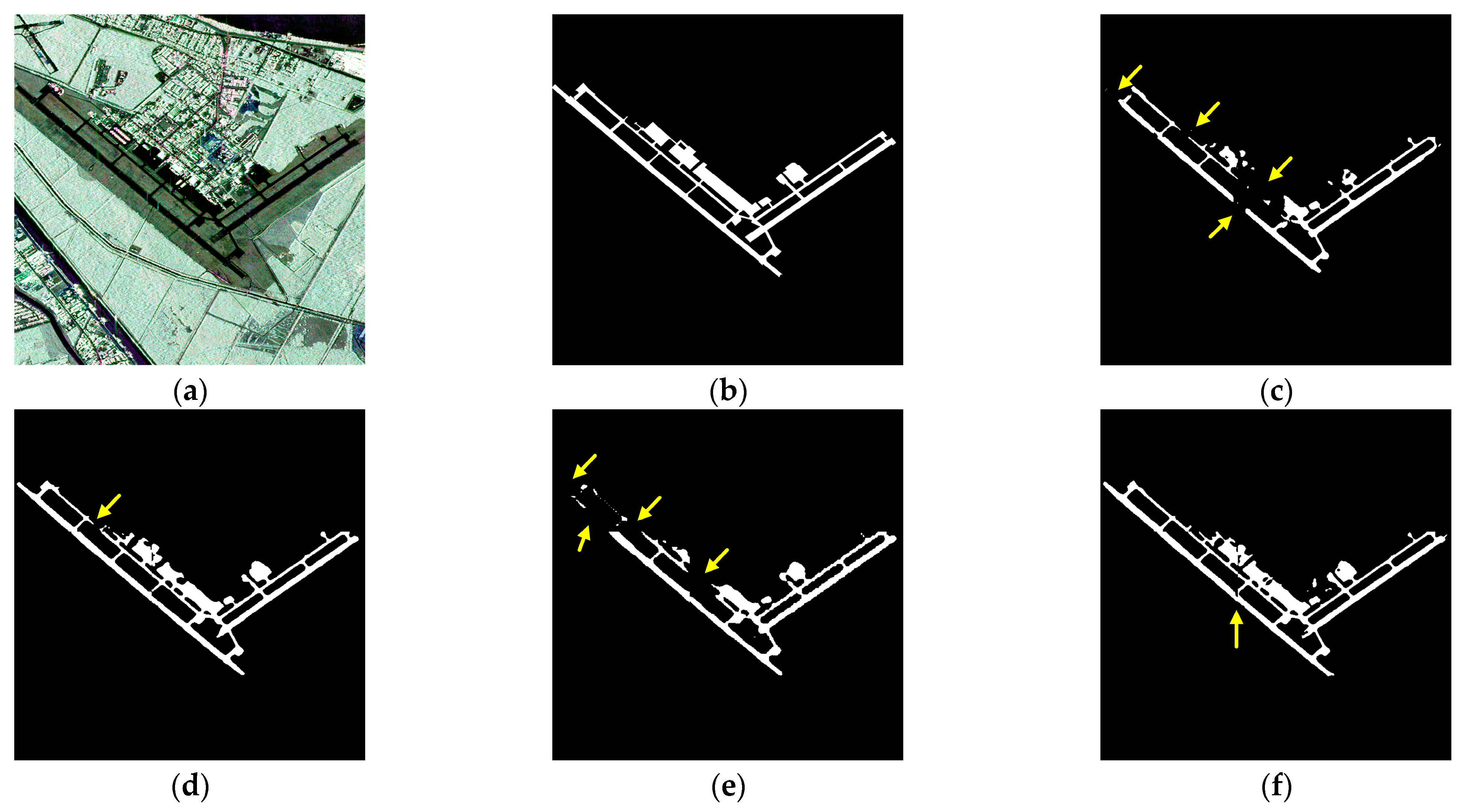
To further validate the effectiveness of our proposed network, we conducted comparative experiments with D-Unet [18], a network specifically designed for airport runway area detection, BA-Net [24], a segmentation network incorporating edge information, and Unet++ [19], a general segmentation network. In all result images, false alarm regions are indicated by green arrows in the complete image, while missed detection regions are indicated by yellow arrows in the enlarged runway area image.
Experiment one was conducted at the New Orleans airport, with image dimensions of 2000 × 2000. The detection results are shown in Figure 24, and the enlarged view of the runway area in the detection results is displayed in Figure 25. As shown in Figure 24a, the yellow box represents the airport area, while the red box indicates objects with similar scattering characteristics, such as rivers, ordinary roads, and mountains, which are highly prone to causing false alarms. In Figure 24c, the Unet++ network fails to distinguish the runway area from the mountainous terrain, regular roads, and other objects with similar characteristics, resulting in a large number of false positives indicated by green arrows. In Figure 25c, both taxiways and the main runway exhibit false negatives. In Figure 24d, the D-Unet network relatively accurately detects the runway area; however, there are a few false positives indicated by the arrows. In Figure 25d, there are a few instances of false negatives in the taxiway area. In Figure 24e, the BA-Net network also shows a few false positives; however, from Figure 25e, it can be observed that there are more severe cases of false negatives, particularly in the taxiway area. In Figure 24f and Figure 25f, it is evident that our proposed method successfully distinguishes the airport runway area from other objects, and the detected contours are relatively complete. Table 3 provides a quantitative comparison of the four methods’ specific metrics in Experiment One. Our method’s PA metric is significantly higher than Unet++ and BA-Net, and it is about 1.6% higher than D-Unet. The Recall metric is slightly lower than D-Unet, about 0.1% lower, mainly due to discontinuities in the detection of the runway area in Figure 25f at the arrow-marked apron area, which is caused by noise interference. It can be seen from Figure 26 that the F1 value and MIoU indicator of this paper are also the highest among the four methods.
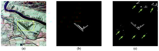

Figure 24.
Compared with the test results of Experiment 1. False alarm regions are indicated by green arrows: (a) PauliRGB Image of New Orleans Airport (The yellow rectangular box represents the airport runway area, while the red rectangular box represents the region that can easily interfere with detection results); (b) Ground truth image; (c) Unet++; (d) D-Unet; (e) BA-Net; (f) SEL-Net (ours).
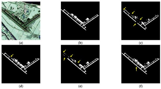
Figure 25.
Enlarged images of runway area detection results from Comparative Experiment 1. Missed detection regions are indicated by yellow arrows: (a) PauliRGB Image of New Orleans Airport; (b) Ground truth image; (c) Unet++; (d) D-Unet; (e) BA-Net; (f) SEL-Net (ours).
Table 3.
Comparing the evaluation index of Experiment 1.
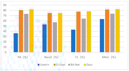
Figure 26.
Bar chart of the evaluation indicators for the comparison experiment 1.
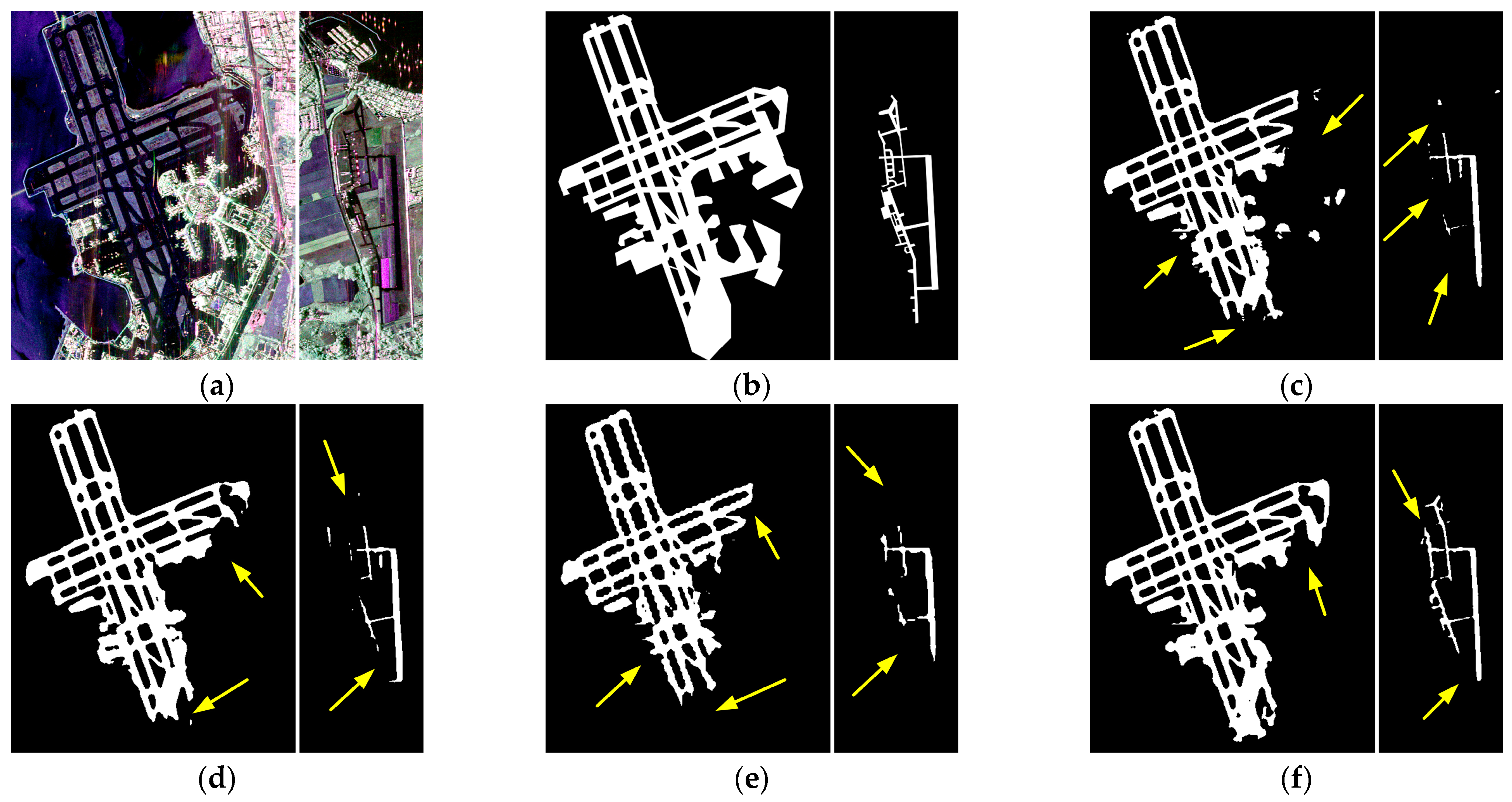
Experiment two was conducted in the San Francisco region, with image dimensions of 3000 × 1500, containing two airports. The detection results are shown in Figure 27, and the enlarged and stitched images of the detected runway areas are presented in Figure 28. As depicted in Figure 27a, the yellow box delineates the airport area, while the red box indicates objects with analogous scattering characteristics, such as lakes, oceans, and mountains, which are highly prone to triggering false alarms. In Figure 27c, the Unet++ network exhibits a few false positives indicated by the green arrows, and in Figure 28c, there are numerous instances of false negatives pointed out by the yellow arrows. In Figure 27d, the D-Unet network shows a few cases of false negatives, and in Figure 28d both airports still have missed detections. Figure 27e demonstrates that the BA-Net network has no false positives in the scene, but from Figure 28e it is apparent that there are more severe cases of false negatives, and the segmentation of runways is not as smooth. In Figure 27f, our proposed method shows no false positives in the scene, and in Figure 28f, the left-side runway detection is relatively complete. There are a few missed detections in both runways, but compared to other methods, our method has fewer instances of missed detections. Additionally, the segmentation of runway areas is more coherent. As shown in Table 4, a quantitative comparison of the specific metrics among the four methods in Experiment Two reveals that our proposed method performs the best in all four metrics. Particularly, the MIoU value is 81.15%, significantly higher than the other three methods. It can be seen from Figure 29 that the four indicators of the method in this paper are optimal.
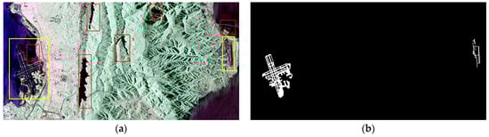
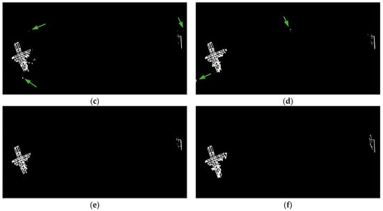
Figure 27.
Compared with the test results of Experiment 2. False alarm regions are indicated by green arrows: (a) PauliRGB imagery of the San Francisco area (The yellow rectangular box represents the airport runway area, while the red rectangular box represents the region that can easily interfere with detection results); (b) Ground truth image; (c) Unet++; (d) D-Unet; (e) BA-Net; (f) SEL-Net (ours).
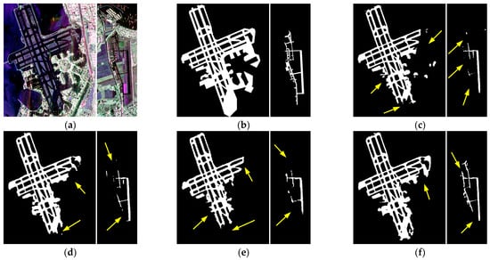
Figure 28.
Enlarged stitched images of runway area detection results from Comparative Experiment 2. Missed detection regions are indicated by yellow arrows: (a) Splicing images of PauliRGB images in the San Francisco area; (b) Ground truth image; (c) Unet++; (d) D-Unet; (e) BA-Net; (f) SEL-Net (ours).
Table 4.
Comparing the evaluation index of Experiment 2.

Figure 29.
Bar chart of the evaluation indicators for the comparison experiment 2.
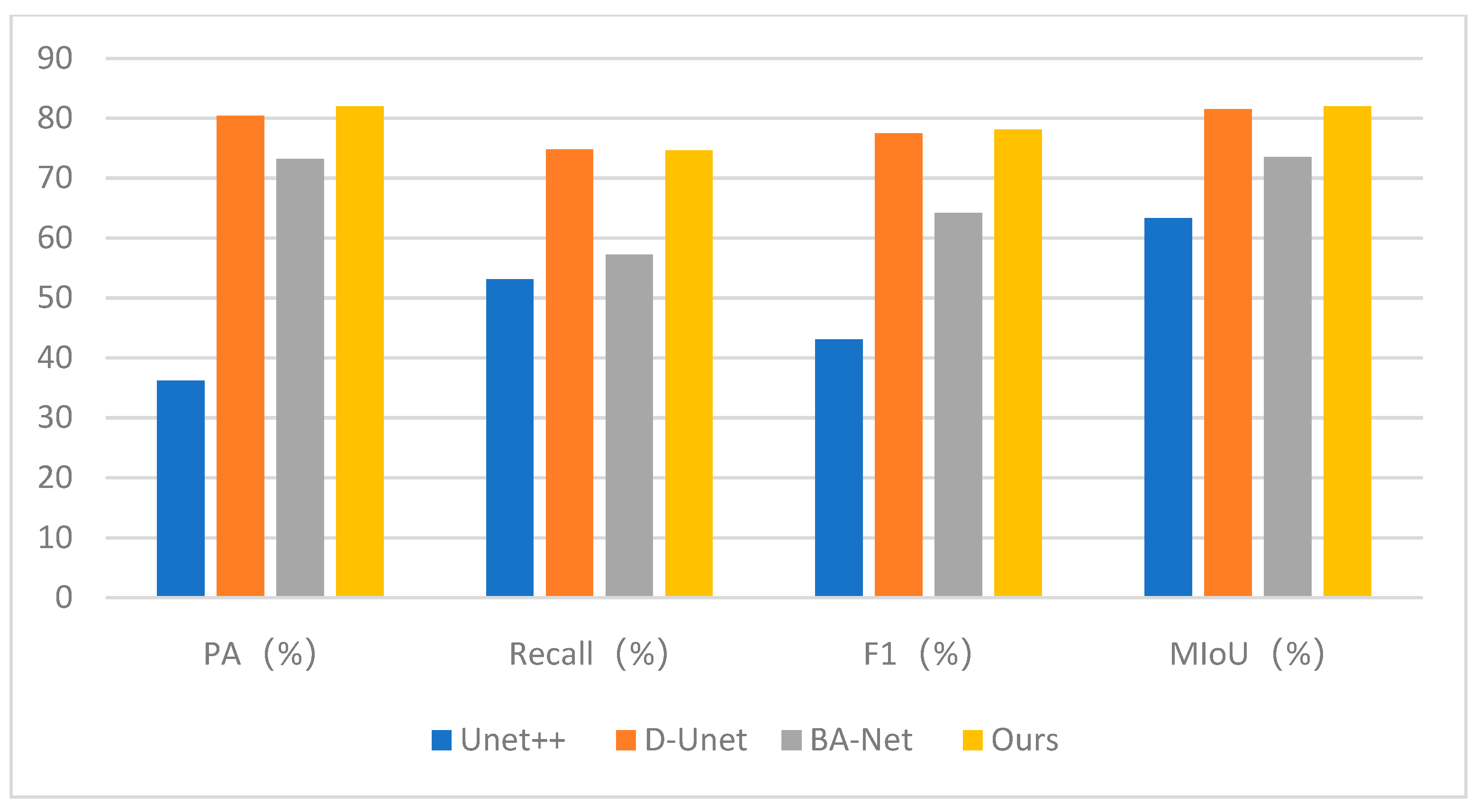
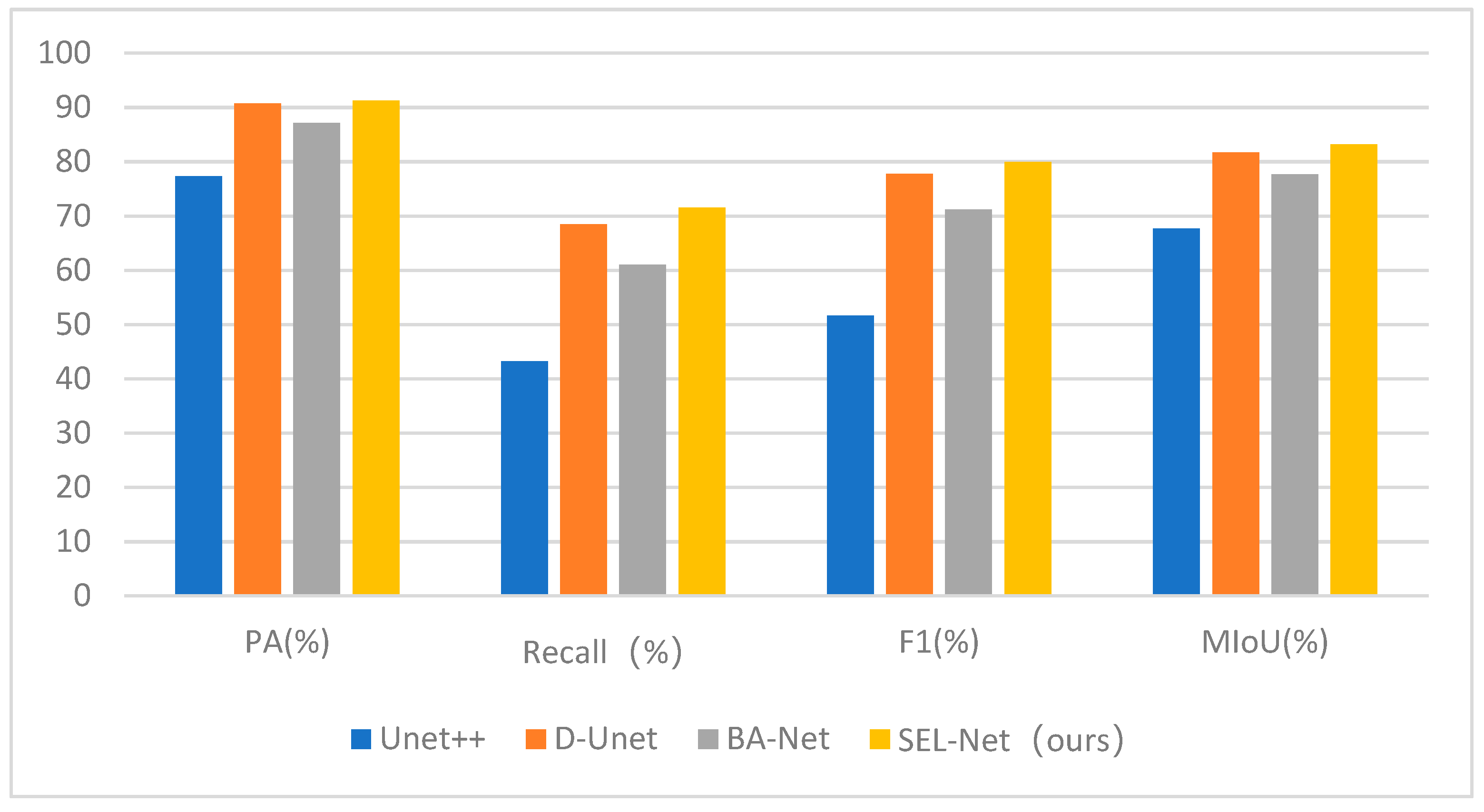
Due to space limitations, the comparative experimental results for other airports in the test sets are not further elaborated. The bar chart in Figure 30 displays the average values of all comparative experiments’ metrics. The specific values for individual metrics can be found in Table 5. It can be observed that our proposed method outperforms the other three networks in all four metrics. The Recall metric slightly surpasses the other three methods by at least 3%, and the average MIoU value is higher than the other three methods by approximately 1.5%. Therefore, it is evident that our proposed method, when achieving good detection performance, has lower false positive and false negative rates compared to other methods. Additionally, the complexity of the network of four methods can be seen from Table 6. This paper performs at a medium level in these three indicators.
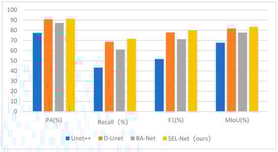
Figure 30.
Comparative chart of average metric values for all test airports.
Table 5.
The average values of the evaluation indicators in the comparative experiments.
Table 6.
Comparison of network complexity indicators in comparative experiments.
5. Discussion
This paper studies how to use self-supervised networks to solve the impact of insufficient PolSAR data annotation on deep learning. In the self-supervised learning stage, feature channel images are added as pseudo-labels and the loss function is improved. It can be seen from the t-SNE dimensionality reduction visualization in Figure 19 and the heat map visualization in Figure 20 that, compared with the previous self-supervised learning methods, the pre-trained model obtained by this paper pays more attention to the extraction of semantic information in the runway area. The ablation experiment in Section 4.4.3 also shows that the introduction of the pre-trained model obtained by self-supervised learning further improves the detection results. In addition, this paper also improves the detection network. It can be seen from the experimental results and channel visualization in the ablation experiment in Section 4.4.3 that the modified model enhances the extraction of edge information and can reduce the loss of semantic information in the network. It can be seen from Table 5 that, in the comparative experiments, this paper’s method is optimal in four evaluation indicators of detection accuracy. It can also be seen from the experimental result figures that this paper’s method has the least false alarm rate, the best runway integrity, and smoother edges compared with other methods. It can be shown that this paper’s method solves the problem of high false alarm rate and runway integrity caused by insufficient extraction of edge information and deep semantic information in the runway area by the network.
Due to the many improvements made to the network to increase accuracy, the complexity of the model has also increased. In the future, there is potential for model lightweighting to enhance detection efficiency while maintaining detection accuracy. Furthermore, as the number of self-supervised learning images used is relatively limited, some feature images may have unclear runway characteristics due to the imaging mechanism. This results in missing imaging in certain areas, leading to slow convergence and higher loss values during self-supervised learning clustering. To address this issue, future work can focus on introducing more polarimetric decomposition methods to obtain feature images with clear runway characteristics. Finally, our network can not only be applied to airport runway area detection, but also can be used in the detection of more similar objects in the future, such as bridge detection. In addition, our network can also be used to detect the linear debris-free glacier parts proposed in the literature [44] to warn of the occurrence of avalanches. Specifically, we can first use a large number of PolSAR images of glacier areas and the feature maps of the features of glaciers and wet snow polarization characteristics proposed in the literature [21] to generate a pre-trained model through self-supervised learning, and then use a small number of labeled images of debris-free glaciers to train the final model to detect the distribution of debris-free glaciers.
6. Conclusions
This paper proposes a self-supervised learning-based PolSAR image runway area detection network called SEL-Net. A pre-trained model is obtained by the self-supervised learning network based on MOCO, and the pre-trained model is transferred to the encoder of the detection network to address the issue of insufficient deep semantic information caused by scarce labeled data during training. The improvement of the downsampling and upsampling structures in the detection network, as well as the inclusion of the STM, solve the problem of semantic information loss during network propagation. The inclusion of the EEM and EFM addresses the issue of insufficient edge information extraction by the network. The resolution of the above issues has led the network to achieve high scores across all four evaluation metrics in comparative experiments. The experimental results demonstrate that the network designed in this study exhibits a high level of accuracy in detecting runway areas in PolSAR images.
Author Contributions
Conceptualization, P.H. and D.L.; Methodology, P.H. and Y.P.; Project administration, P.H. and B.H.; Software, P.H., Y.P. and Z.C.; Validation, Y.P., Z.C. and B.H.; Visualization, Y.P. and D.L.; Writing—original draft, P.H. and Y.P.; Writing—review & editing, P.H., Y.P., Z.C. and D.L. All authors have read and agreed to the published version of the manuscript.
Funding
This research was funded by Research and Development Fund of Civil Aviation University of China, grant number 2015/6221042. The APC was funded by Research and Development Fund of Civil Aviation University of China.
Data Availability Statement
Not applicable.
Conflicts of Interest
The authors declare no conflict of interest.
References
- Zhang, D. Talking about the Importance and Significance of General Aviation Airport Construction. Sci. Technol. Ind. Parks 2017, 15, 233. [Google Scholar]
- Xu, X.; Zou, B.; Zhang, L. PolSAR Image Classification Based on Object-Based Markov Random Field with Polarimetric Auxiliary Label Field. IEEE Trans. Geosci. Remote Sens. 2019, 17, 1558–1562. [Google Scholar] [CrossRef]
- Jin, K.; Chen, Y.; Xu, B.; Yin, J.; Wang, X.; Yang, J. A Patch-to-Pixel Convolutional Neural Network for Small Ship Detection with PolSAR Images. IEEE Trans. Geosci. Remote Sens. 2020, 58, 6623–6638. [Google Scholar] [CrossRef]
- Liu, F.; Duan, Y.; Li, L.; Jiao, L.; Wu, J.; Yang, S.; Zhang, X.; Yuan, J. SAR Image Segmentation Based on Hierarchical Visual Semantic and Adaptive Neighborhood Multinomial Latent Model. IEEE Trans. Geosci. Remote Sens. 2016, 54, 4287–4301. [Google Scholar] [CrossRef]
- Cui, Y.; Liu, F.; Liu, X.; Li, L.; Qian, X. TCSPANET: Two-Staged Contrastive Learning and Sub-Patch Attention Based Network for Polsar Image Classification. Remote Sens. 2022, 14, 2451. [Google Scholar] [CrossRef]
- Ji, C.; Cheng, L.; Li, N.; Zeng, F.; Li, M. Validation of Global Airport Spatial Locations from Open Databases Using Deep Learning for Runway Detection. IEEE J. Sel. Top. Appl. Earth Obs. Remote Sens. 2020, 14, 1120–1131. [Google Scholar] [CrossRef]
- Tu, J.; Gao, F.; Sun, J.; Hussain, A.; Zhou, H. Airport Detection in SAR Images via Salient Line Segment Detector and Edge-Oriented Region Growing. IEEE J. Sel. Top. Appl. Earth Obs. Remote Sens. 2020, 14, 314–326. [Google Scholar] [CrossRef]
- Liu, N.; Cui, Z.; Cao, Z.; Pi, Y.; Dang, S. Airport Detection in Large-Scale SAR Images via Line Segment Grouping and Saliency Analysis. IEEE Trans. Geosci. Remote Sens. 2018, 15, 434–438. [Google Scholar] [CrossRef]
- Ai, S.; Yan, J.; Li, D. Airport Runway Detection Algorithm in Remote Sensing Images. Electron. Opt. Control. 2017, 24, 43–46. [Google Scholar]
- Marapareddy, R.; Pothuraju, A. Runway Detection Using Unsupervised Classification. In Proceedings of the 2017 IEEE 8th Annual Ubiquitous Computing, Electronics and Mobile Communication Conference (UEMCON), New York, NY, USA, 19–21 October 2017; IEEE: New York, NY, USA, 2017; pp. 278–281. [Google Scholar]
- Lu, X.; Lin, Z.; Han, P.; Zou, C. Fast Detection of Airport Runway Areas in PolSAR Images Using Adaptive Unsupervised Classification. Natl. Remote Sens. Bull. 2019, 23, 1186–1193. [Google Scholar] [CrossRef]
- Han, P.; Liu, Y.; Han, B.; Chen, Z. Airport Runway Area Detection in PolSAR Image Combined with Image Segmentation and Classification. J. Signal Process. 2021, 37, 2084–2096. [Google Scholar]
- Zhang, Z.; Zou, C.; Han, P.; Lu, X. A Runway Detection Method Based on Classification Using Optimized Polarimetric Features and HOG Features for PolSAR Images. IEEE Access 2020, 8, 49160–49168. [Google Scholar] [CrossRef]
- Liu, N.; Cao, Z.; Cui, Z.; Pi, Y.; Dang, S. Multi-Layer Abstraction Saliency for Airport Detection in SAR Images. IEEE Trans. Geosci. Remote Sens. 2019, 57, 9820–9831. [Google Scholar] [CrossRef]
- Zhao, D.; Li, J.; Shi, Z.; Jiang, Z.; Meng, C. Subjective Saliency Model Driven by Multi-Cues Stimulus for Airport Detection. IEEE Access 2019, 7, 32118–32127. [Google Scholar] [CrossRef]
- Zhang, Y.; Zhu, W.; Xing, Q. A Survey of SAR Image Segmentation Methods. J. Ordnance Equip. Eng. 2017, 38, 99–103. [Google Scholar]
- Ronneberger, O.; Fischer, P.; Brox, T. U-Net: Convolutional Networks for Biomedical Image Segmentation. In Proceedings of the Medical Image Computing and Computer-Assisted Intervention–MICCAI, Singapore, 18–22 September 2022; Springer: Munich, Germany, 2015; pp. 234–241. [Google Scholar]
- Han, P.; Liang, Y. Airport Runway Area Segmentation in PolSAR Image Based D-Unet Network. In Proceedings of the International Workshop on ATM/CNS, Tokyo, Japan, 25–27 October 2022; Electronic Navigation Research Institute: Tokyo, Japan, 2022; pp. 127–136. [Google Scholar]
- Zhou, Z.; Rahman Siddiquee, M.M.; Tajbakhsh, N.; Liang, J. Unet++: A Nested u-Net Architecture for Medical Image Segmentation. In Proceedings of the Deep Learning in Medical Image Analysis and Multimodal Learning for Clinical Decision Support: 4th International Workshop, DLMIA 2018, Granada, Spain, 20 September 2018; Springer: Granada, Spain, 2018; pp. 3–11. [Google Scholar]
- Chen, L.-C.; Papandreou, G.; Schroff, F.; Adam, H. Rethinking Atrous Convolution for Semantic Image Segmentation. Arxiv Prepr. 2017, arXiv:1706.05587. [Google Scholar]
- Usami, N.; Muhuri, A.; Bhattacharya, A.; Hirose, A. Proposal of Wet Snowmapping with Focus on Incident Angle Influential to Depolarization of Surface Scattering. In Proceedings of the 2016 IEEE International Geoscience and Remote Sensing Symposium (IGARSS), Beijing, China, 10–15 July 2016; IEEE: Beijing, China, 2016; pp. 1544–1547. [Google Scholar]
- Shang, F.; Hirose, A. Quaternion Neural-Network-Based PolSAR Land Classification in Poincare-Sphere-Parameter Space. IEEE Trans. Geosci. Remote Sens. 2014, 52, 5693–5703. [Google Scholar] [CrossRef]
- Tan, S.; Chen, L.; Pan, Z.; Xing, J.; Li, Z.; Yuan, Z. Geospatial Contextual Attention Mechanism for Automatic and Fast Airport Detection in SAR Imagery. IEEE Access 2020, 8, 173627–173640. [Google Scholar] [CrossRef]
- Wang, R.; Chen, S.; Ji, C.; Fan, J.; Li, Y. Boundary-Aware Context Neural Network for Medical Image Segmentation. Med. Image Anal. 2022, 78, 102395. [Google Scholar] [CrossRef]
- Du, S.; Li, W.; Xing, J.; Zhang, C.; She, C.; Wang, S. Change detection of open-pit mining area based on FM-UNet++ and Gaofen-2 satellite images. Coal Geol. Explor. 2023, 51, 1–12. [Google Scholar]
- Wang, C.; Wang, S.; Chen, X.; Li, J.; Xie, T. Object-level change detection in multi-source optical remote sensing images combined with UNet++ and multi-level difference modules. Acta Geod. Cartogr. Sin. 2023, 52, 283–296. [Google Scholar]
- Du, Y.; Zhong, R.; Li, Q.; Zhang, F. TransUNet++ SAR: Change Detection with Deep Learning about Architectural Ensemble in SAR Images. Remote Sens. 2022, 15, 6. [Google Scholar] [CrossRef]
- Peng, C.; Zhang, X.; Yu, G.; Luo, G.; Sun, J. Large Kernel Matters–Improve Semantic Segmentation by Global Convolutional Network. In Proceedings of the IEEE Conference on Computer Vision and Pattern Recognition (CVPR), Honolulu, HI, USA, 21–26 July 2017; pp. 4353–4361. [Google Scholar]
- Zhang, Z.; Zhang, X.; Peng, C.; Xue, X.; Sun, J. Exfuse: Enhancing Feature Fusion for Semantic Segmentation. In Proceedings of the Proceedings of the European Conference on Computer Vision (ECCV), Munich, Germany, 8–14 September 2018; pp. 269–284. [Google Scholar]
- Gu, Z.; Cheng, J.; Fu, H.; Zhou, K.; Hao, H.; Zhao, Y.; Zhang, T.; Gao, S.; Liu, J. Ce-Net: Context Encoder Network for 2d Medical Image Segmentation. IEEE Trans. Med. Imaging 2019, 38, 2281–2292. [Google Scholar] [CrossRef] [PubMed]
- Xu, Q.; Ma, Z.; Na, H.E.; Duan, W. DCSAU-Net: A Deeper and More Compact Split-Attention U-Net for Medical Image Segmentation. Comput. Biol. Med. 2023, 154, 106626. [Google Scholar] [CrossRef] [PubMed]
- Szegedy, C.; Vanhoucke, V.; Ioffe, S.; Shlens, J.; Wojna, Z. Rethinking the Inception Architecture for Computer Vision. In Proceedings of the IEEE Conference on Computer Vision and Pattern Recognition (CVPR), Las Vegas, NV, USA, 26 June 2016; pp. 2818–2826. [Google Scholar]
- Han, P.; Liu, Y.; Cheng, Z. Airport Runway Detection Based on a Combination of Complex Convolution and ResNet for PolSAR Images. In Proceedings of the 2021 SAR in Big Data Era (BIGSARDATA), Nanjing, China, 22 September 2021; pp. 1–4. [Google Scholar]
- He, K.; Fan, H.; Wu, Y.; Xie, S.; Girshick, R. Momentum Contrast for Unsupervised Visual Representation Learning. In Proceedings of the IEEE/CVF Conference on Computer Vision and Pattern Recognition (CVPR), Seattle, WA, USA, 14 June 2020; pp. 9729–9738. [Google Scholar]
- Zhang, L.; Zhang, S.; Zou, B.; Dong, H. Unsupervised Deep Representation Learning and Few-Shot Classification of PolSAR Images. IEEE Trans. Geosci. Remote Sens. 2020, 60, 1–16. [Google Scholar] [CrossRef]
- Chen, T.; Kornblith, S.; Norouzi, M.; Hinton, G. A Simple Framework for Contrastive Learning of Visual Representations. In Proceedings of the International Conference on Machine Learning (PMLR), Vienna, Austria, 12 July 2020; pp. 1597–1607. [Google Scholar]
- Zhang, C.; Chen, J.; Li, Q.; Deng, B.; Wang, J.; Chen, C. A Survey of Deep Contrastive Learning. Acta Autom. Sin. 2023, 49, 15–39. [Google Scholar] [CrossRef]
- Fu, J.; Liu, J.; Tian, H.; Li, Y.; Bao, Y.; Fang, Z.; Lu, H. Dual Attention Network for Scene Segmentation. In Proceedings of the IEEE/CVF Conference on Computer Vision and Pattern Recognition (CVPR), Long Beach, CA, USA, 16 June 2019; pp. 3146–3154. [Google Scholar]
- Wu, T.; Tang, S.; Zhang, R.; Cao, J.; Zhang, Y. Cgnet: A Light-Weight Context Guided Network for Semantic Segmentation. IEEE Trans. Image Process. 2020, 30, 1169–1179. [Google Scholar] [CrossRef]
- Yu, C.; Wang, J.; Peng, C.; Gao, C.; Yu, G.; Sang, N. Learning a Discriminative Feature Network for Semantic Segmentation. In Proceedings of the IEEE Conference on Computer Vision and Pattern Recognition (CVPR), Salt Lake City, UT, USA, 18 June 2018; pp. 1857–1866. [Google Scholar]
- Takikawa, T.; Acuna, D.; Jampani, V.; Fidler, S. Gated-Scnn: Gated Shape Cnns for Semantic Segmentation. In Proceedings of the IEEE/CVF International Conference on Computer Vision (ICCV), Seoul, Republic of Korea, 27 October 2019; pp. 5229–5238. [Google Scholar]
- Lee, J.-S.; Pottier, E. Polarimetric Radar Imaging: From Basics to Applications; CRC Press: Boca Raton, FL, USA, 2017. [Google Scholar]
- Huynen, J.R. Stokes Matrix Parameters and Their Interpretation in Terms of Physical Target Properties. In Proceedings of the Polarimetry: Radar, Infrared, Visible, Ultraviolet, and X-ray, Huntsville, AL, USA, 15–17 May 1990; SPIE: Huntsville, AL, USA, 1990; Volume 1317, pp. 195–207. [Google Scholar]
- Shugar, D.H.; Jacquemart, M.; Shean, D.; Bhushan, S.; Upadhyay, K.; Sattar, A.; Schwanghart, W.; McBride, S.; De Vries, M.V.W.; Mergili, M.; et al. A Massive Rock and Ice Avalanche Caused the 2021 Disaster at Chamoli, Indian Himalaya. Science 2021, 373, 300–306. [Google Scholar] [CrossRef]


Disclaimer/Publisher’s Note: The statements, opinions and data contained in all publications are solely those of the individual author(s) and contributor(s) and not of MDPI and/or the editor(s). MDPI and/or the editor(s) disclaim responsibility for any injury to people or property resulting from any ideas, methods, instructions or products referred to in the content. |
© 2023 by the authors. Licensee MDPI, Basel, Switzerland. This article is an open access article distributed under the terms and conditions of the Creative Commons Attribution (CC BY) license (https://creativecommons.org/licenses/by/4.0/).