
Estimating Agricultural Cropping Intensity Using a New Temporal Mixture Analysis Method from Time Series MODIS


Abstract
:
1. Introduction
2. Materials and Methods
2.1. Study Area and Data
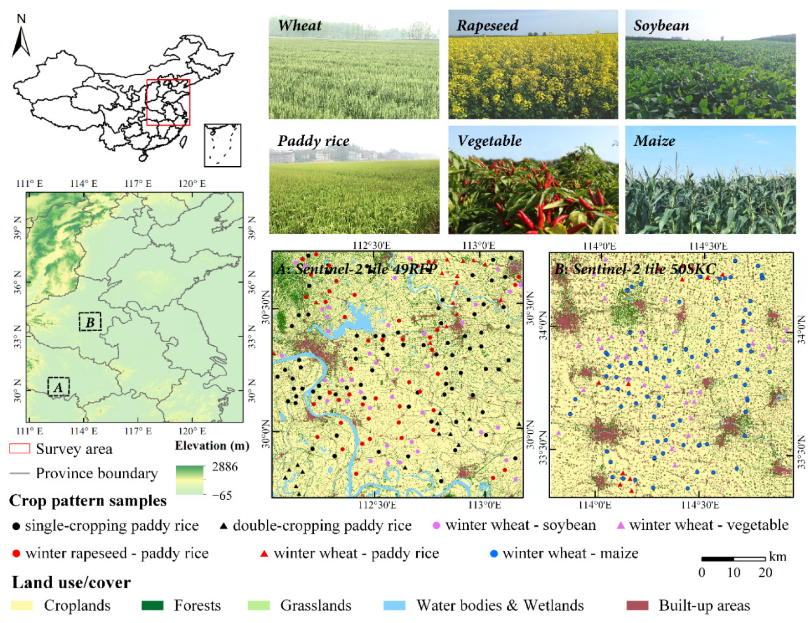
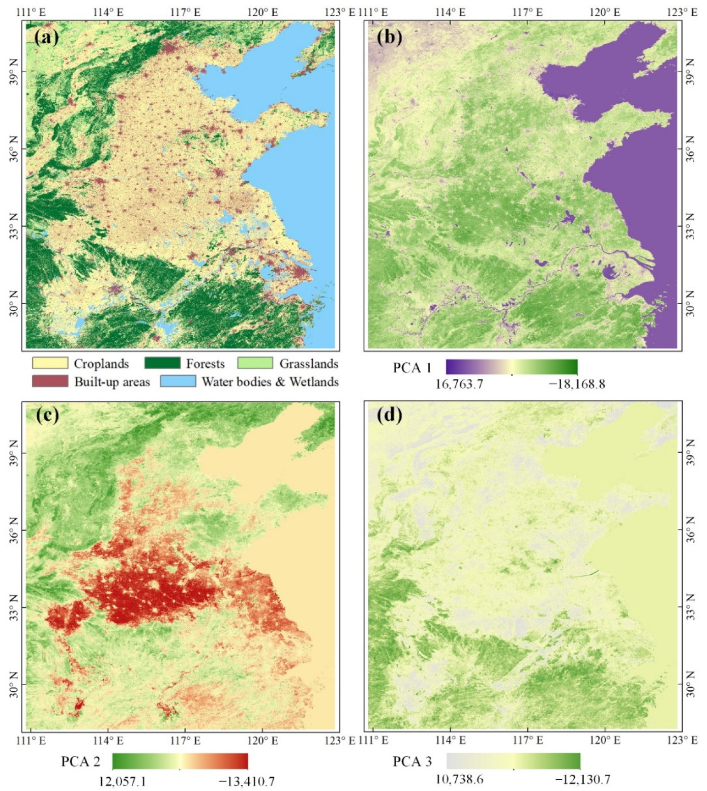
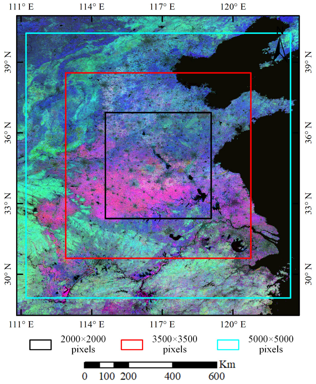
2.1.1. Study Area
2.1.2. Data
2.2. Methods
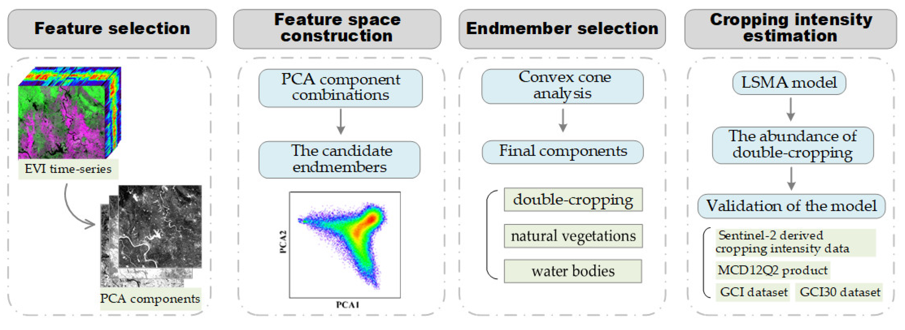
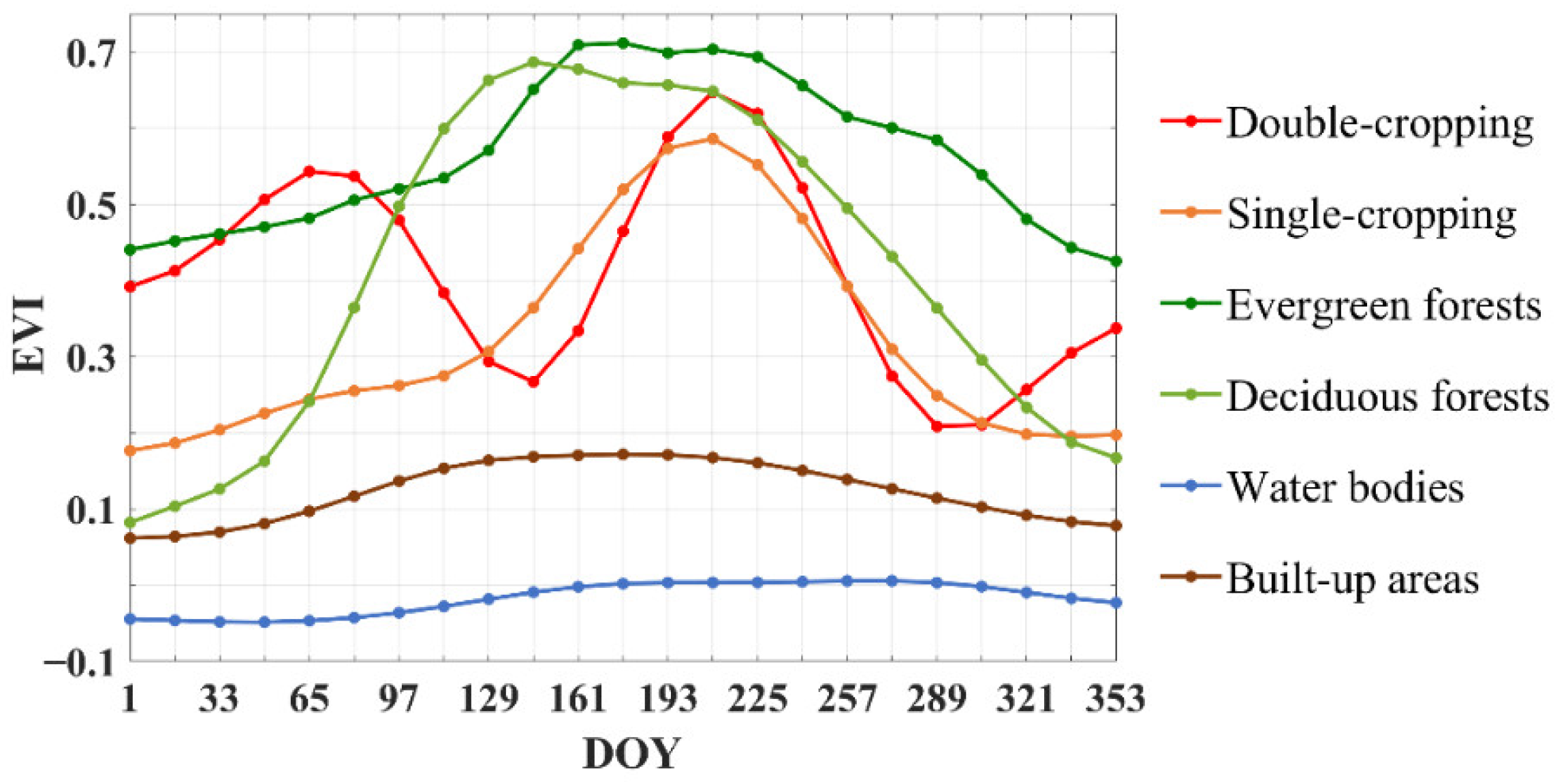
2.2.1. Feature Selection
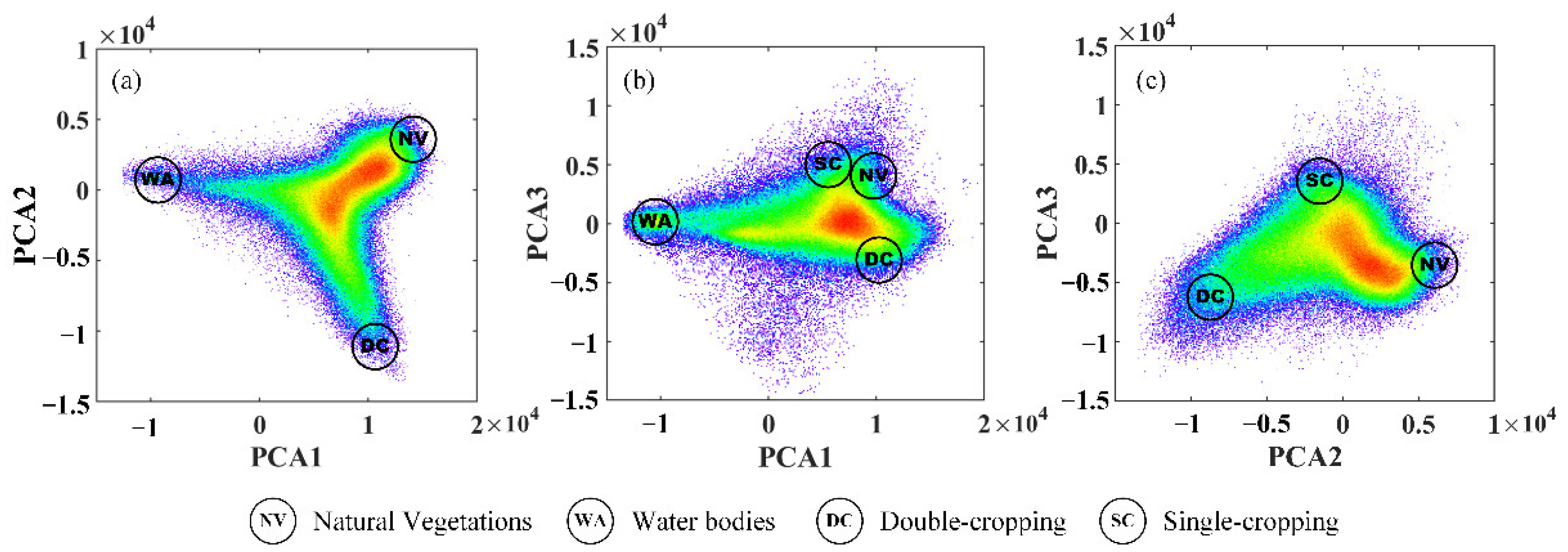
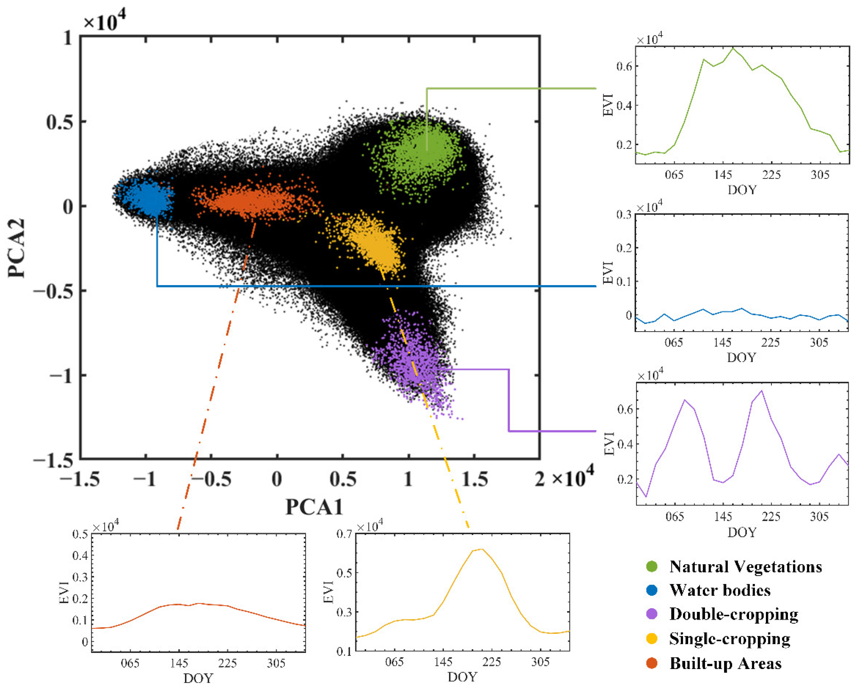
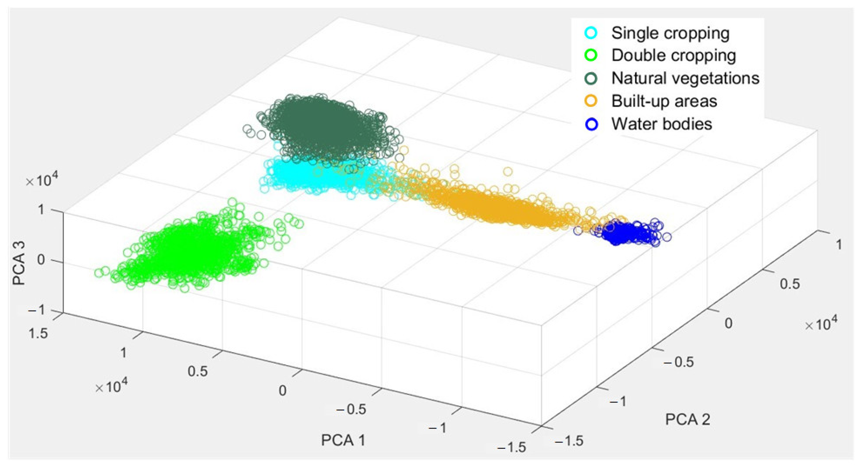
2.2.2. Feature Space Construction and Endmember Selection
2.2.3. Cropping Intensity Estimation
2.2.4. Validation of the Model
3. Results
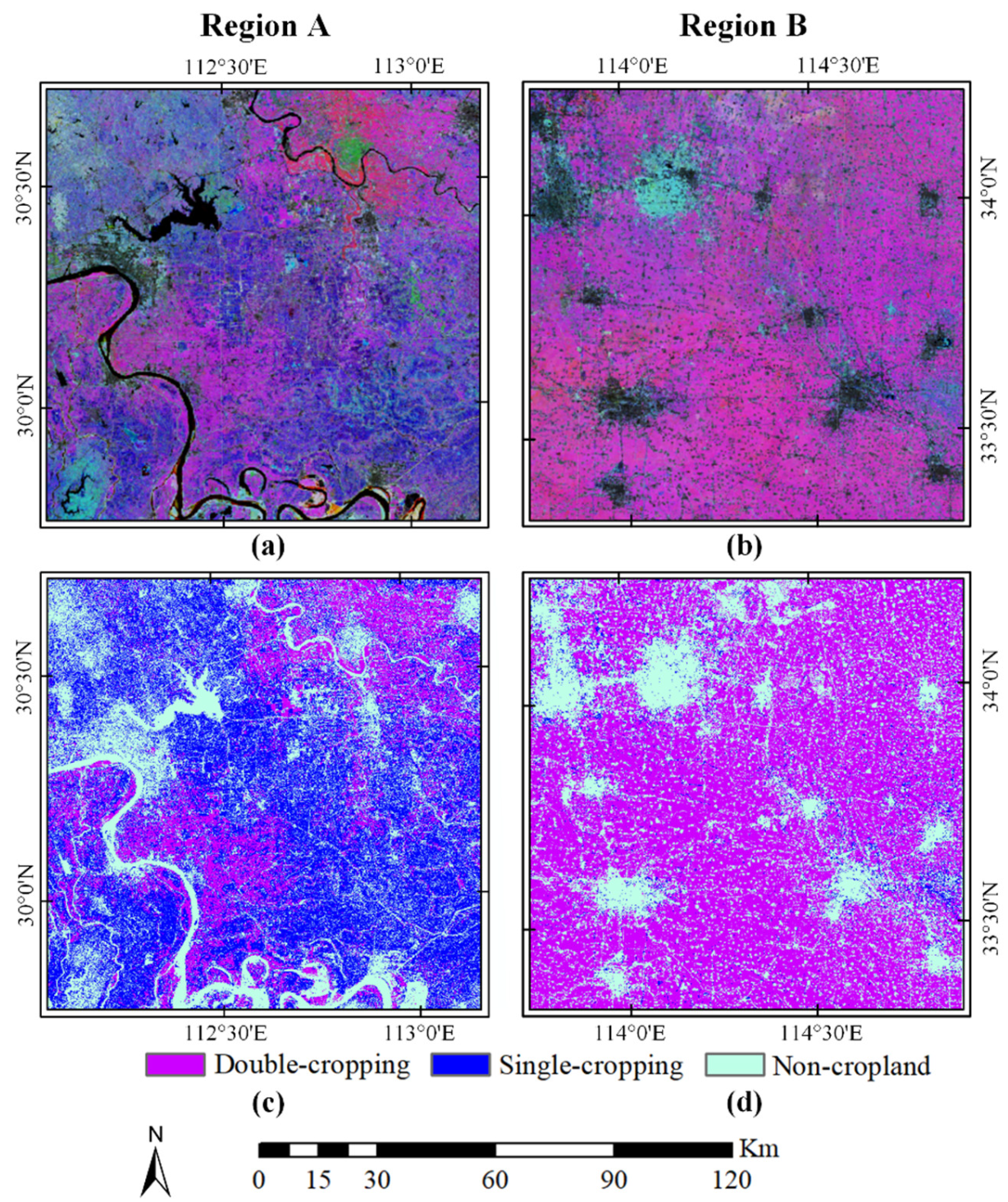
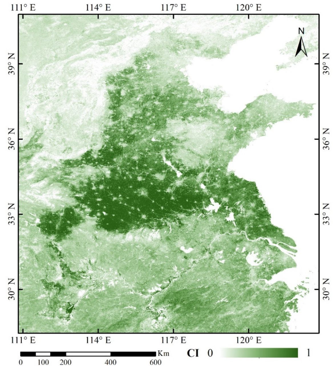
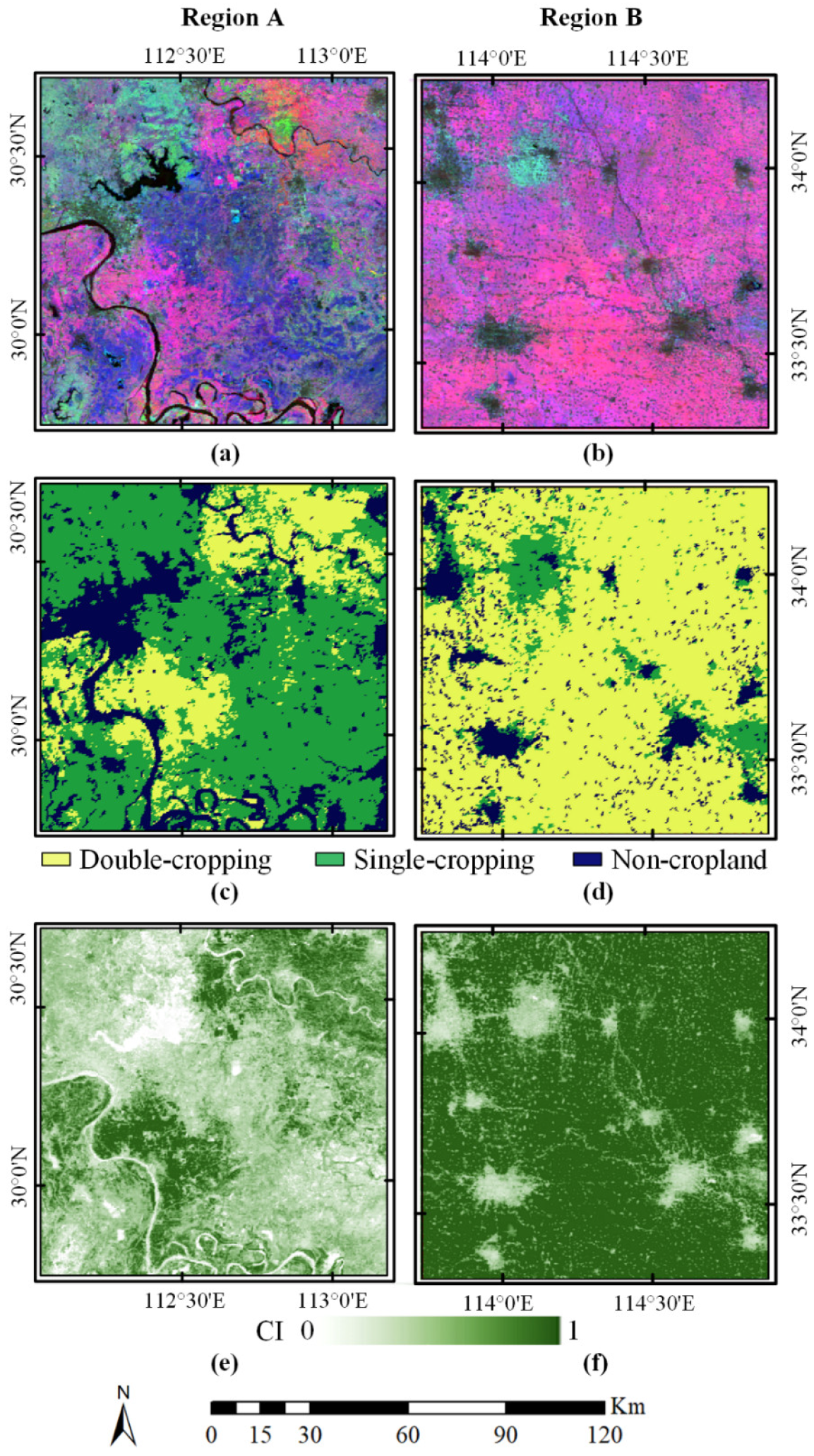
3.1. Cropping Intensity Map
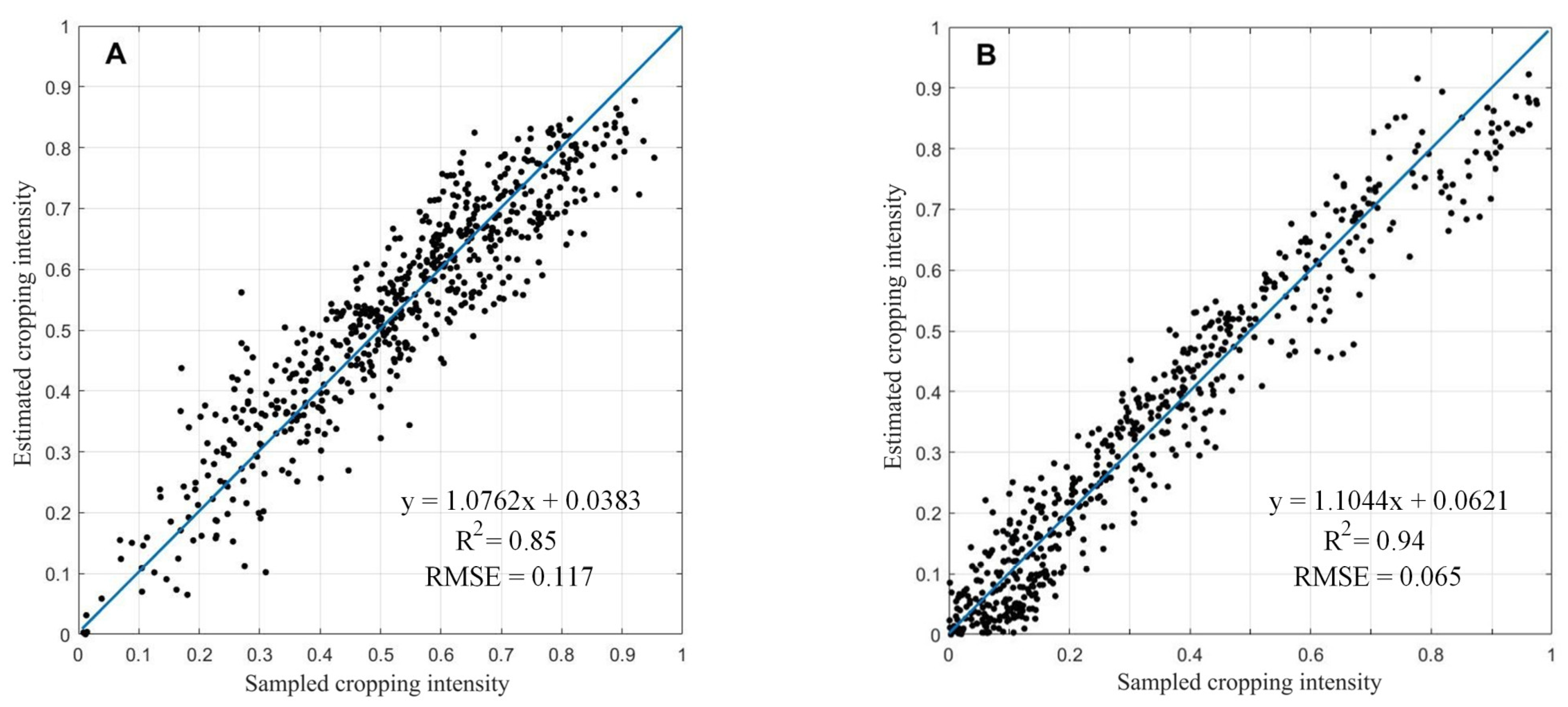
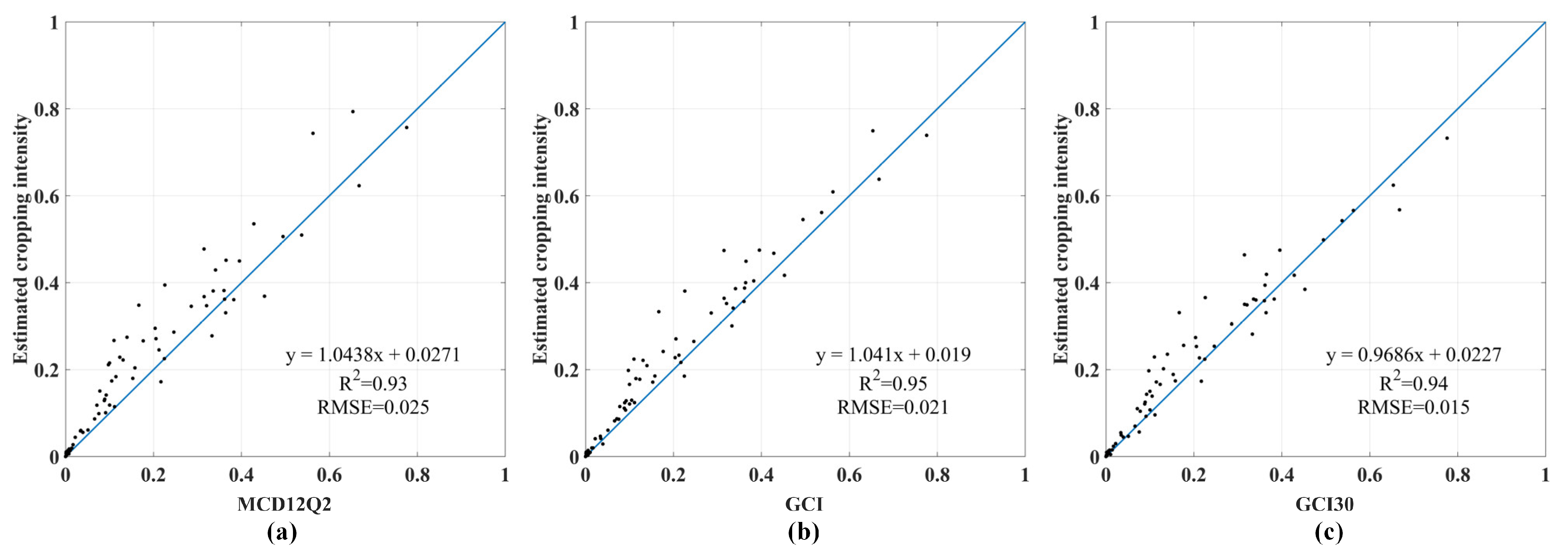
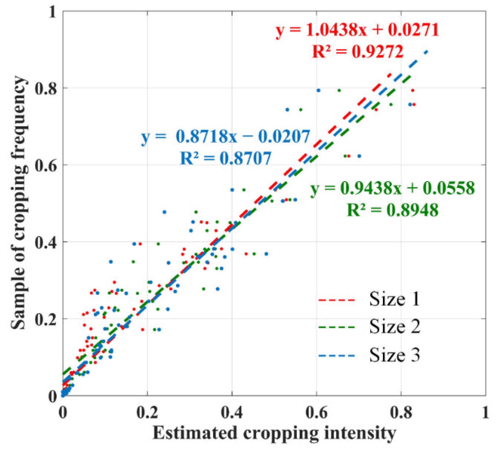
3.2. Validation Results
4. Discussions
4.1. Determining the Final Endmembers
4.2. Delineating the Endmembers Manually
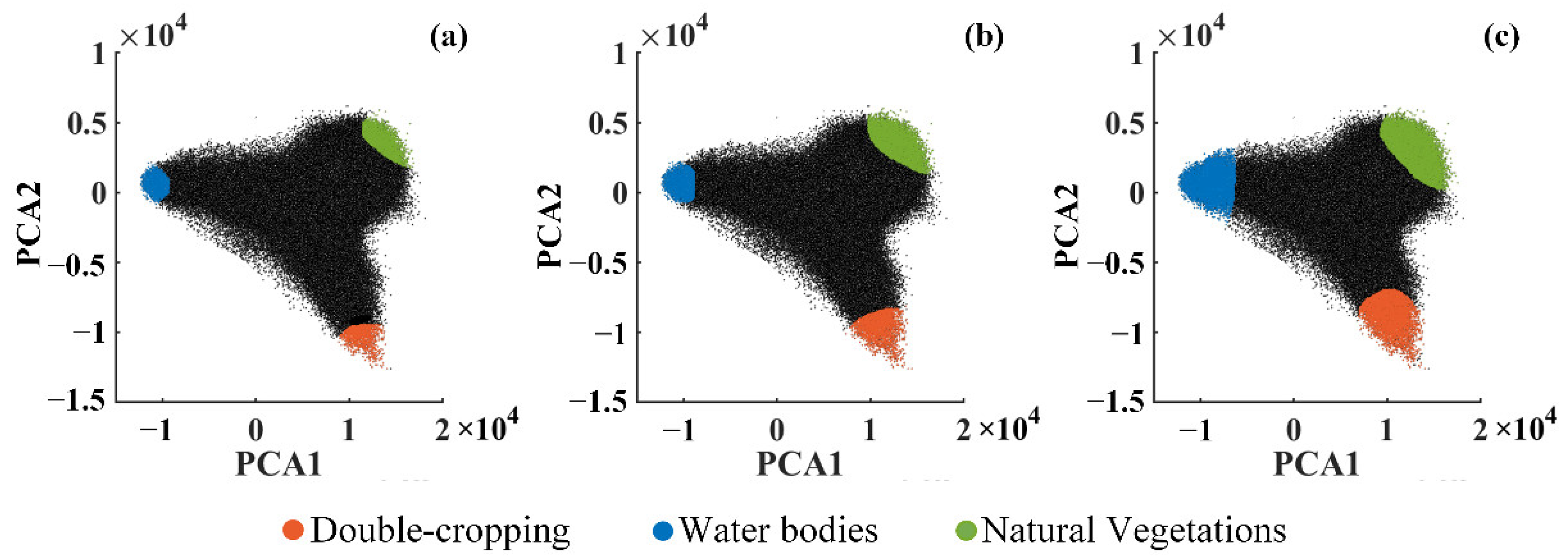
4.3. Unmixing in Regions with Different Sizes and Varied Endmember Land-Cover Types
5. Conclusions
Author Contributions
Funding
Data Availability Statement
Acknowledgments
Conflicts of Interest
References
- Zhu, H.; Sun, M. Main progress in the research on land use intensification. Acta Geogr. Sin. 2014, 69, 1346–1357. [Google Scholar]
- Liu, G.; Zhang, L.; Zhang, Q.; Musyimi, Z. The response of grain production to changes in quantity and quality of cropland in yangtze river delta, China. J. Sci. Food Agric. 2015, 95, 480–489. [Google Scholar] [CrossRef]
- Liu, J.; Kuang, W.; Zhang, Z.; Xu, X.; Qin, Y.; Ning, J.; Zhou, W.; Zhang, S.; Li, R.; Yan, C.; et al. Spatiotemporal characteristics, patterns, and causes of land-use changes in China since the late 1980s. J. Geogr. Sci. 2014, 24, 195–210. [Google Scholar] [CrossRef]
- Tao, J.; Wang, Y.; Qiu, B.; Wu, W. Exploring cropping intensity dynamics by integrating crop phenology information using bayesian networks. Comput. Electron. Agric. 2022, 193, 106667. [Google Scholar] [CrossRef]
- Su, Y.; Qian, K.; Lin, L.; Wang, K.; Guan, T.; Gan, M. Identifying the driving forces of non-grain production expansion in rural China and its implications for policies on cultivated land protection. Land Use Policy 2020, 92, 104435. [Google Scholar] [CrossRef]
- Liu, X.; Herbert, S.J. Fifteen years of research examining cultivation of continuous soybean in northeast China: A review. Field Crops Res. 2002, 79, 1–7. [Google Scholar] [CrossRef]
- Sun, J.; Mooney, H.; Wu, W.; Tang, H.; Tong, Y.; Xu, Z.; Huang, B.; Cheng, Y.; Yang, X.; Wei, D.; et al. Importing food damages domestic environment: Evidence from global soybean trade. Proc. Natl. Acad. Sci. USA 2018, 115, 5415–5419. [Google Scholar] [CrossRef]
- Li, S.; Li, X.; Sun, L.; Cao, G.; Fischer, G.; Tramberend, S. An estimation of the extent of cropland abandonment in mountainous regions of China. Land Degrad. Dev. 2018, 29, 1327–1342. [Google Scholar] [CrossRef]
- Peng, W.; Ma, N.L.; Zhang, D.; Zhou, Q.; Yue, X.; Khoo, S.C.; Yang, H.; Guan, R.; Chen, H.; Zhang, X. A review of historical and recent locust outbreaks: Links to global warming, food security and mitigation strategies. Environ. Res. 2020, 191, 110046. [Google Scholar] [CrossRef]
- Mottaleb, K.A.; Kruseman, G.; Snapp, S. Potential impacts of ukraine-russia armed conflict on global wheat food security: A quantitative exploration. Glob. Food Secur. 2022, 35, 100659. [Google Scholar] [CrossRef]
- Rahimi, P.; Islam, M.S.; Duarte, P.M.; Tazerji, S.S.; Sobur, M.A.; El Zowalaty, M.E.; Ashour, H.M.; Rahman, M.T. Impact of the COVID-19 pandemic on food production and animal health. Trends Food Sci. Technol. 2022, 121, 105–113. [Google Scholar] [CrossRef] [PubMed]
- Yu, X.; Liu, C.; Wang, H.; Feil, J.-H. The impact of COVID-19 on food prices in China: Evidence of four major food products from beijing, shandong and hubei provinces. China Agric. Econ. Rev. 2020, 12, 445–458. [Google Scholar] [CrossRef]
- Dongyu, Q. Role and Potential of Potato in Global Food Security; FAO: Rome, Italy, 2022. [Google Scholar]
- Liu, W.; Yang, H.; Liu, Y.; Kummu, M.; Hoekstra, A.Y.; Liu, J.; Schulin, R. Water resources conservation and nitrogen pollution reduction under global food trade and agricultural intensification. Sci. Total Environ. 2018, 633, 1591–1601. [Google Scholar] [CrossRef] [PubMed]
- Rachele, R. Briefing-Desertification and Agriculture; European Parliament: Strasbourg, France, 2020. [Google Scholar]
- Xu, B.; Niu, Y.; Zhang, Y.; Chen, Z.; Zhang, L. China’s agricultural non-point source pollution and green growth: Interaction and spatial spillover. Environ. Sci. Pollut. Res. 2022, 29, 60278–60288. [Google Scholar] [CrossRef] [PubMed]
- Liu, Y.; Tang, H.; Muhammad, A.; Huang, G. Emission mechanism and reduction countermeasures of agricultural greenhouse gases—A review. Greenh. Gases Sci. Technol. 2019, 9, 160–174. [Google Scholar] [CrossRef]
- Xie, H.; Liu, G. Spatiotemporal difference and determinants of multiple cropping index in China during 1998–2012. Acta Geogr. Sin. 2015, 70, 604–614. [Google Scholar]
- Guo, Y.; Xia, H.; Pan, L.; Zhao, X.; Li, R. Mapping the northern limit of double cropping using a phenology-based algorithm and google earth engine. Remote Sens. 2022, 14, 1004. [Google Scholar] [CrossRef]
- Jiang, M.; Xin, L.; Li, X.; Tan, M.; Wang, R. Decreasing rice cropping intensity in southern China from 1990 to 2015. Remote Sens. 2019, 11, 35. [Google Scholar] [CrossRef]
- Löw, F.; Biradar, C.; Dubovyk, O.; Fliemann, E.; Akramkhanov, A.; Narvaez Vallejo, A.; Waldner, F. Regional-scale monitoring of cropland intensity and productivity with multi-source satellite image time series. Gisci. Remote Sens. 2018, 55, 539–567. [Google Scholar] [CrossRef]
- Qiu, B.; Lu, D.; Tang, Z.; Song, D.; Zeng, Y.; Wang, Z.; Chen, C.; Chen, N.; Huang, H.; Xu, W. Mapping cropping intensity trends in China during 1982–2013. Appl. Geogr. 2017, 79, 212–222. [Google Scholar] [CrossRef]
- Yan, H.; Liu, F.; Qin, Y.; Doughty, R.; Xiao, X. Tracking the spatio-temporal change of cropping intensity in China during 2000–2015. Environ. Res. Lett. 2019, 14, 035008. [Google Scholar] [CrossRef]
- Pan, L.; Xia, H.; Yang, J.; Niu, W.; Qin, Y. Mapping cropping intensity in huaihe basin using phenology algorithm, all sentinel-2 and landsat images in google earth engine. Int. J. Appl. Earth Obs. Geoinf. 2021, 102, 102376. [Google Scholar] [CrossRef]
- Liu, L.; Xiao, X.; Qin, Y.; Wang, J.; Xu, X.; Hu, Y.; Qiao, Z. Mapping cropping intensity in China using time series landsat and sentinel-2 images and google earth engine. Remote Sens. Environ. 2020, 239, 111624. [Google Scholar] [CrossRef]
- Liu, C.; Zhang, Q.; Tao, S.; Qi, J.; Ding, M.; Guan, Q.; Wu, B.; Zhang, M.; Nabil, M.; Tian, F. A new framework to map fine resolution cropping intensity across the globe: Algorithm, validation, and implication. Remote Sens. Environ. 2020, 251, 112095. [Google Scholar] [CrossRef]
- Tao, J.; Wu, W.; Xu, M. Using the bayesian network to map large-scale cropping intensity by fusing multi-source data. Remote Sens. 2019, 11, 168. [Google Scholar] [CrossRef]
- Tao, J.; Wu, W.; Liu, W. Spatial-temporal dynamics of cropping frequency in hubei province over 2001–2015. Sensors 2017, 17, 2622. [Google Scholar] [CrossRef]
- Qiu, B.; Li, W.; Tang, Z.; Chen, C.; Qi, W. Mapping paddy rice areas based on vegetation phenology and surface moisture conditions. Ecol. Indic. 2015, 56, 79–86. [Google Scholar] [CrossRef]
- Tian, H.F.; Huang, N.; Niu, Z.; Qin, Y.C.; Pei, J.; Wang, J. Mapping winter crops in China with multi-source satellite imagery and phenology-based algorithm. Remote Sens. 2019, 11, 820. [Google Scholar] [CrossRef]
- d’Andrimont, R.; Taymans, M.; Lemoine, G.; Ceglar, A.; Yordanov, M.; van der Velde, M. Detecting flowering phenology in oil seed rape parcels with sentinel-1 and-2 time series. Remote Sens. Environ. 2020, 239, 111660. [Google Scholar] [CrossRef]
- Pok, S.; Matsushita, B.; Fukushima, T. An easily implemented method to estimate impervious surface area on a large scale from modis time-series and improved dmsp-ols nighttime light data. ISPRS J. Photogramm. Remote Sens. 2017, 133, 104–115. [Google Scholar] [CrossRef]
- Chen, Y.; Yun, W.; Zhou, X.; Peng, J.; Li, S.; Zhou, Y. Classification and extraction of land use information in hilly area based on mesma and rf classifier. Trans. Chin. Soc. Agric. Mach 2017, 48, 136–144. [Google Scholar]
- Ridd, M.K. Exploring a vis (vegetation-impervious surface-soil) model for urban ecosystem analysis through remote sensing: Comparative anatomy for cities. Int. J. Remote Sens. 1995, 16, 2165–2185. [Google Scholar] [CrossRef]
- Ji, C.; Li, X.; Wei, H.; Li, S. Comparison of different multispectral sensors for photosynthetic and non-photosynthetic vegetation-fraction retrieval. Remote Sens. 2020, 12, 115. [Google Scholar] [CrossRef]
- Pi, X.; Zeng, Y.; He, C. High-resolution urban vegetation coverage estimation based on multi-source remote sensing data fusion. Natl. Remote Sens. Bull. 2021, 25, 1216–1226. [Google Scholar] [CrossRef]
- Wang, Y.; Zhuo, R.; Xu, L.; Fang, Y. A spatial-temporal bayesian deep image prior model for moderate resolution imaging spectroradiometer temporal mixture analysis. Remote Sens. 2023, 15, 3782. [Google Scholar] [CrossRef]
- Caballero, I.; Stumpf, R.P. Towards routine mapping of shallow bathymetry in environments with variable turbidity: Contribution of sentinel-2a/b satellites mission. Remote Sens. 2020, 12, 451. [Google Scholar] [CrossRef]
- Gray, J.; Sulla-Menashe, D.; Friedl, M.A. User Guide to Collection 6 Modis Land Cover Dynamics (mcd12q2) Product. In NASA EOSDIS Land Process; DAAC: Missoula, MT, USA, 2019; Volume 6, pp. 1–8. [Google Scholar]
- Liu, X.; Zheng, J.; Yu, L.; Hao, P.; Chen, B.; Xin, Q.; Fu, H.; Gong, P. Annual dynamic dataset of global cropping intensity from 2001 to 2019. Sci. Data 2021, 8, 283. [Google Scholar] [CrossRef]
- Zhang, M.; Wu, B.; Zeng, H.; He, G.; Liu, C.; Tao, S.; Zhang, Q.; Nabil, M.; Tian, F.; Bofana, J. Gci30: A global dataset of 30 m cropping intensity using multisource remote sensing imagery. Earth Syst. Sci. Data 2021, 13, 4799–4817. [Google Scholar] [CrossRef]
- Boardman, J.W. Automated Spectral Unmixing of Aviris Data Using Convex Geometry Concepts. In Proceedings of the Jplairborne Geoscience Workshop, Washington, DC, USA, 25–29 October 1993. [Google Scholar]
- Melaas, E.K.; Friedl, M.A.; Zhu, Z. Detecting interannual variation in deciduous broadleaf forest phenology using landsat tm/etm+ data. Remote Sens. Environ. 2013, 132, 176–185. [Google Scholar] [CrossRef]
- Bellón, B.; Bégué, A.; Seen, D.L.; Almeida, C.A.d.; Simões, M. A remote sensing approach for regional-scale mapping of agricultural land-use systems based on ndvi time series. Remote Sens. 2017, 9, 600. [Google Scholar] [CrossRef]
- Henderson, C.; Petersen, K.; Redak, R. Spatial and temporal patterns in the seed bank and vegetation of a desert grassland community. J. Ecol. 1988, 76, 717–728. [Google Scholar] [CrossRef]
- Wang, T.; Kou, X.; Xiong, Y.; Mou, P.; Wu, J.; Ge, J. Temporal and spatial patterns of ndvi and their relationship to precipitation in the loess plateau of China. Int. J. Remote Sens. 2010, 31, 1943–1958. [Google Scholar] [CrossRef]
- Yang, C.; Wu, G.; Ding, K.; Shi, T.; Li, Q.; Wang, J. Improving land use/land cover classification by integrating pixel unmixing and decision tree methods. Remote Sens. 2017, 9, 1222. [Google Scholar] [CrossRef]
- Singh, R.; Kumar, V. Evaluating automated endmember extraction for classifying hyperspectral data and deriving spectral parameters for monitoring forest vegetation health. Environ. Monit. Assess. 2022, 195, 72. [Google Scholar] [CrossRef]
- Wang, H.; Wu, B.; Li, X.; Lu, S. Extraction of impervious surface in hai basin using remote sensing. J. Remote Sens. 2011, 15, 388–400. (In Chinese) [Google Scholar]

| Cropping Intensity | Single-Cropping | Double-Cropping | Other | Total | UA (%) |
|---|---|---|---|---|---|
| single-cropping | 489 | 28 | 12 | 529 | 92.44 |
| double-cropping | 42 | 567 | 17 | 626 | 90.58 |
| other | 6 | 27 | 591 | 624 | 94.71 |
| total | 537 | 622 | 620 | 1779 | |
| PA (%) | 91.06 | 91.16 | 95.32 | OA = 0.926 Kappa = 0.888 |
| Number of Features | Features | Types of Models | Endmembers |
|---|---|---|---|
| 1 | PCA 2 | two-endmember model | double-cropping, natural vegetation, |
| 2 | PCA 1, PCA 3 | two-endmember model | double-cropping, water bodies |
| 2 | PCA 1, PCA 2 | three-endmember model | double-cropping, natural vegetation, water bodies |
| 2 | PCA 2, PCA 3 | three-endmember model | double-cropping, single-cropping, natural vegetation |
| 3 | PCA 1, PCA 2, PCA 3 | four-endmember model | double-cropping, single-cropping, natural vegetation, water bodies |
| Area Size (Pixels) | Feature Space | R2 |
| 2000 × 2000 | 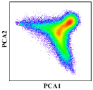 | 0.9358 |
| 3500 × 3500 | 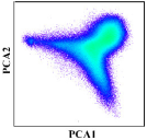 | 0.8747 |
| 5000 × 5000 | 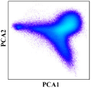 | 0.9034 |
| Endmembers | MODIS False-Color Composite (DOY 065, 145, 065) | Feature Space | Completeness of Endmembers |
|---|---|---|---|
| double-cropping, water bodies | 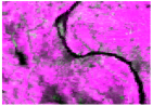 | 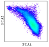 | No |
| double-cropping, natural vegetation | 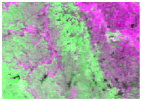 |  | No |
| natural vegetation, water bodies | 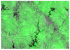 |  | No |
| double-cropping, natural vegetation, water bodies | 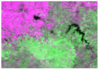 |  | Yes |
Disclaimer/Publisher’s Note: The statements, opinions and data contained in all publications are solely those of the individual author(s) and contributor(s) and not of MDPI and/or the editor(s). MDPI and/or the editor(s) disclaim responsibility for any injury to people or property resulting from any ideas, methods, instructions or products referred to in the content. |
© 2023 by the authors. Licensee MDPI, Basel, Switzerland. This article is an open access article distributed under the terms and conditions of the Creative Commons Attribution (CC BY) license (https://creativecommons.org/licenses/by/4.0/).
Share and Cite
Tao, J.; Zhang, X.; Liu, Y.; Jiang, Q.; Zhou, Y. Estimating Agricultural Cropping Intensity Using a New Temporal Mixture Analysis Method from Time Series MODIS. Remote Sens. 2023, 15, 4712. https://doi.org/10.3390/rs15194712
Tao J, Zhang X, Liu Y, Jiang Q, Zhou Y. Estimating Agricultural Cropping Intensity Using a New Temporal Mixture Analysis Method from Time Series MODIS. Remote Sensing. 2023; 15(19):4712. https://doi.org/10.3390/rs15194712
Chicago/Turabian StyleTao, Jianbin, Xinyue Zhang, Yiqing Liu, Qiyue Jiang, and Yang Zhou. 2023. "Estimating Agricultural Cropping Intensity Using a New Temporal Mixture Analysis Method from Time Series MODIS" Remote Sensing 15, no. 19: 4712. https://doi.org/10.3390/rs15194712
APA StyleTao, J., Zhang, X., Liu, Y., Jiang, Q., & Zhou, Y. (2023). Estimating Agricultural Cropping Intensity Using a New Temporal Mixture Analysis Method from Time Series MODIS. Remote Sensing, 15(19), 4712. https://doi.org/10.3390/rs15194712