On-Earth Observation of Low Earth Orbit Targets through Phase Disturbances by Atmospheric Turbulence

Abstract

This paper addresses the challenges of ground-based observation of Low Earth Orbit (LEO) targets using on-Earth telescopes and proposes solutions for improving image quality and tracking fast-moving objects under atmospheric turbulence conditions. The study investigates major challenges, including atmospheric turbulence-induced aberrations, blurring, telescope platform vibrations, and spatial variations caused by the target motion. A scenario simulation is conducted considering practical limitations, such as feasible time slots for monitoring and the number of available frames within the Field of View (FoV). The paper proposes a novel method for detecting LEO targets using Harris corner features and matching adjacent images upon the corrected frames by Adaptive Optics (AO), with a $38\%$ reduction in the Mean Squared Error (MSE) achieved for certain frames within the isoplanatic angle. Additionally, a refinement strategy for deblurring images is proposed, combining the post-processing with Singular Value Decomposition (SVD) filtering; with a proper filtering factor ($\beta =0.1$), an almost complete collection of 14 corner nodes can be detected. The feasibility of continuously tracking objects with uncontrolled attitudes, such as space debris, is successfully demonstrated with continuous monitoring of certain features. The proposed methods offer promising solutions for ground-based observation of LEO targets, providing insights for further research and application in this field.

1. Introduction

Ground-based observation of Low Earth Orbit (LEO) targets presents significant challenges due to atmospheric turbulence, platform vibrations, and the motion of the tracked object. These challenges limit the quality of acquired images and hinder effective tracking of fast-moving objects [1]. However, the ability to observe and track LEO targets using on-Earth telescopes holds great importance for various applications, such as space surveillance and orbital debris monitoring. Overcoming these challenges and improving image quality are crucial for enhancing our understanding of LEO objects and their behaviors [2,3]. Large apertures enable the collection of more light from faint celestial bodies and allow for more accurate observations with higher resolution. However, ground environments often make this ideal situation unattainable. The Earth’s atmosphere alters the light from space through two distinct phenomena. First, there is wavelength-dependent filtering, allowing only optical/near-infrared and radio electromagnetic waves to reach the Earth’s surface. The second limiting factor is atmospheric turbulence [4], which causes random variations in the refractive index of the air. This induces temporal and spatial random wavefront errors and can lead to phenomena like twinkling or scintillation of stars during night observations, which further worsens the viewing conditions. In this case, the angular resolution is limited by the seeing given by $\lambda /r_0$, where $r_0$ is the Fried coherence length [5]. This parameter physically represents the aperture size that has the same resolution as a diffraction-limited aperture in the absence of atmospheric turbulence.

To address these challenges, various techniques have been proposed, such as Adaptive Optics (AO) [6], which aims at compensating for atmospheric turbulence in real-time, correcting the wavefront aberrations and improving image qualities; it requires hardware implementation with Deformable Mirrors (DMs) and a wavefront sensor. The AO technique is commonly used in large ground telescopes for astronomical observations, transferring a seeing-limited telescope into a diffraction-limited one. However, it is important to note that the requirements for tracking LEO objects and conducting astronomical observations of stationary stars or planets are quite different:

• LEO targets are fast-moving, which means that the imaging process can only be performed in a short time with several consecutive frames captured. The received photons may not be sufficient for generating high-quality images. In contrast, observations of stationary stars often involve long exposure times [7]. Additionally, the motion-induced blurring of LEO object images needs to be filtered out.
• In the realm of astronomical observations, the traditional approach hinges on stars as the primary sources of light, with cameras adeptly accumulating substantial energy over the long exposure time. Stars, by their nature, commonly serve as Natural Guide Stars (NGS) for AO systems, providing the essential input for the wavefront sensor [4]. In contrast, fast-moving objects at LEO typically adopt a passive stance, devoid of any intrinsic light emission. These objects come into view only when they catch and reflect sunlight back toward the Earth observer, offering limited observation opportunities within specific time windows.
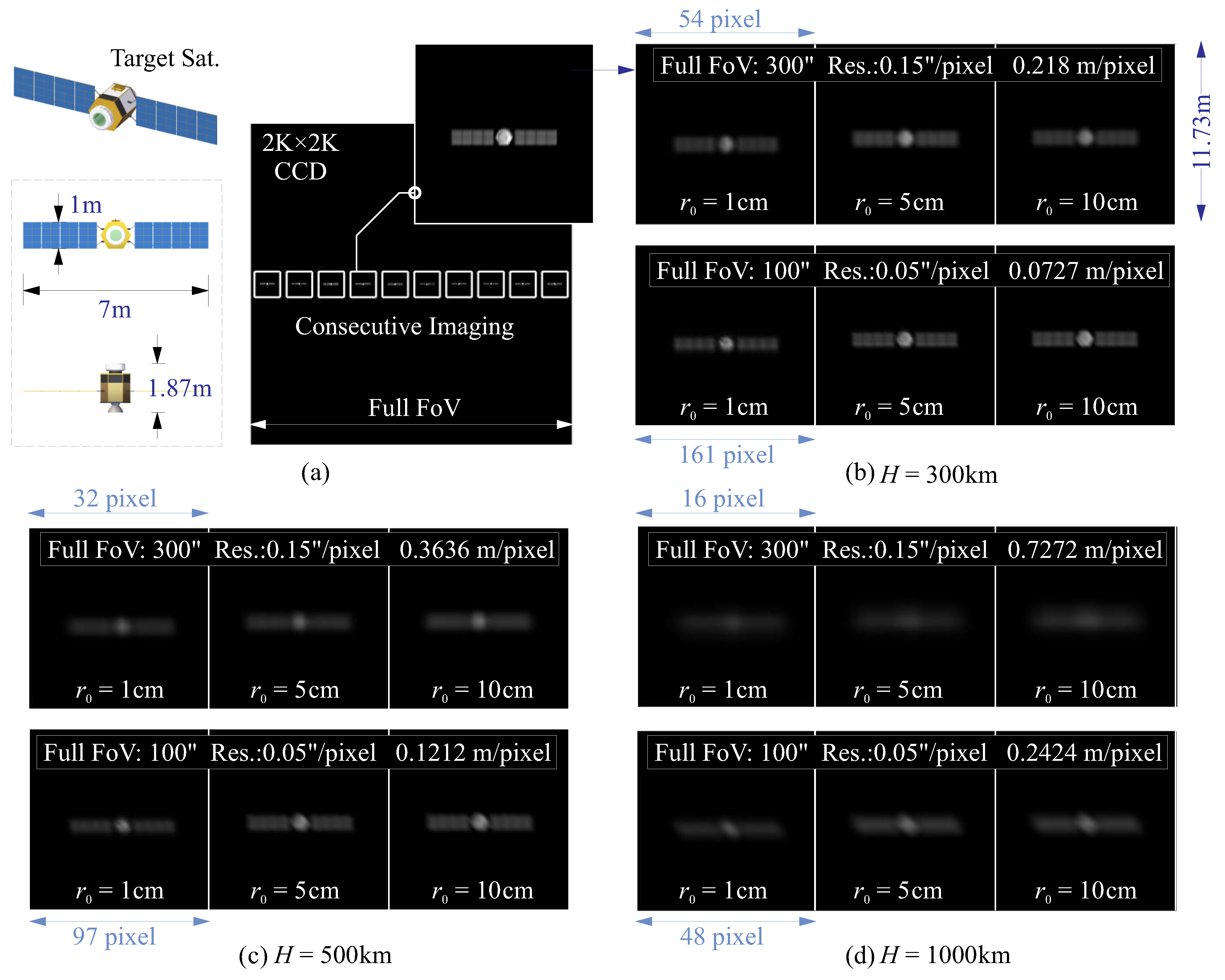
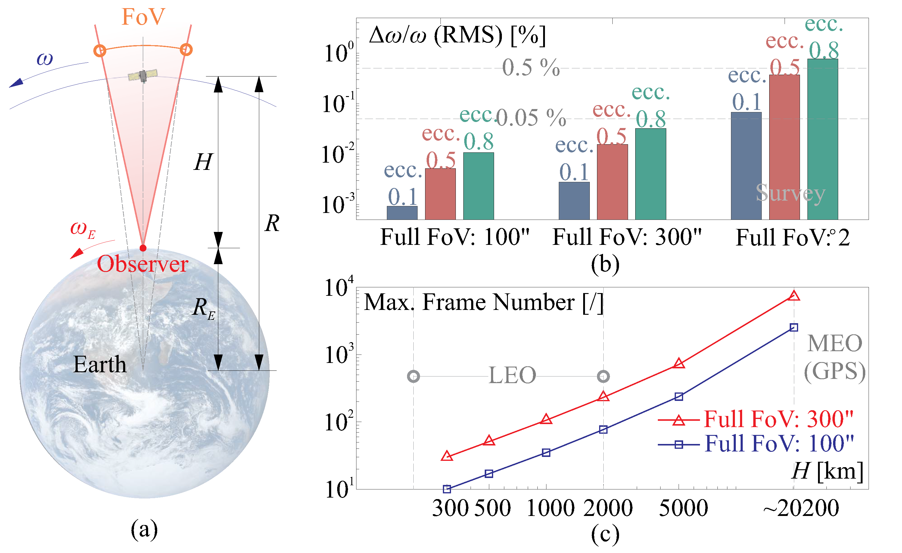
• Stationary stars or planets remain almost unchanged in the camera view if the motion of the Earth’s rotation is compensated during night observation. The observed region in the night sky is often narrow, allowing the telescope to be pointed to a specific direction for an extended period. Moreover, the targets typically occupy a large field within the observation area. However, monitoring LEO objects is entirely different; these LEO moving objects are usually tiny in the FoV. For instance, a 10 m satellite at an orbital height of $H=800$ km has an angular view of only 2.6 arcsec, while Jupiter is 35 arcsec wide, and Sirius A and B vary from 3 to 11 arcsec. Furthermore, LEO objects move across a very large region, making telescope tracking extremely challenging.
• When using AO correction, the corrected field is usually sufficient for observing a single astronomical target. However, achieving this on a fast-moving LEO object is difficult, as very few frames can be deblurred with the corrected wavefront during the imaging process.

The primary objective of monitoring LEO objects is to facilitate space surveillance and enhance situational awareness. Consequently, a specific focus is placed on examining on-structure features, which can be refined through post-processing techniques. In this context, achieving exceptional image quality takes precedence as a fundamental requirement for effective monitoring and in-depth analysis. Historically, radio detection has been the dominant method for tracking LEO objects, as evidenced by prior studies [8]. However, when dealing with objects in LEO within the optical range, a multitude of challenges surface, as previously discussed. Recent efforts have been initiated to detect LEO objects from ground-based stations, primarily for ranging and imaging purposes [1,9]. Furthermore, there is a reasonable expectation of significant enhancements in observation capabilities through the implementation of AO systems. Records from publicly available resources validate the early use of AO for monitoring satellites, primarily for military purposes, as exemplified by the Starfire Optical Range (SOR) [10,11,12] and the Advanced Electro-Optical System (AEOS) [13], initiated by the US Air Force. Over the past few years, this field has witnessed substantial growth, marked by advancements in hardware [14] and the launch of significant projects [15,16,17].

This paper discusses various aspects of the challenges associated with ground-based observation of LEO targets and presents solutions for observing such objects using on-Earth telescopes. The study is numerically conducted with a MATLAB-platform toolbox. The paper is organized as follows: Section 2 reports the modeling of the optical phase delays using a three-layer structure of atmospheric frozen screens, each driven by independent wind velocities. The resulting phase aberrations at the telescope’s entrance pupil are generated by summing those layered screens; the spatial structure of the overall phase aberration is analyzed using modal coordinates of Zernike polynomials, and the temporal spectra of decomposed coefficients are analyzed. In addition, the effect of optical tilts is also examined through the blob analysis. Section 3 simulates the scenario of ground observation of rapid moving LEO objects, considering feasible time slots for monitoring and the numbers of available frames within the FoV during the imaging process; the access opportunities for the observation task are assessed. The study also proposes a method for detecting LEO targets by identifying Harris corner features in consecutive frames and matching adjacent images, and the deteriorating effect of atmosphere is discussed. Section 4 develops a refinement strategy for deblurring the images, combining the AO hardware implementation and post-processing using SVD filtering for the frame set. The observation of objects with uncontrolled attitudes (e.g., space debris) is also explored, demonstrating the feasibility of continuously tracking these objects under the influence of atmospheric disturbances using the proposed method of AO correction with SVD filtering. Notice that, in this paper, we develop the frame formation process virtually and, thus, image qualities might be better than practical acquisition since some real-world factors are ignored except for the atmospheric turbulence.

2. Deteriorated Observation by Atmospheric Turbulence and Platform Condition

Several considerations are involved in the design of the architecture for the on-Earth observation of LEO objects, as depicted in the figure. Firstly, the LEO objects being detected typically occupy a small field for observation, which requires a telescope with a large focal length ($f_L$) to achieve better pixel resolution. The pixel resolution $L_P$ (in a unit of m/pixel) can be calculated using the geometric relation, according to the theory of paraxial optics,

$$L_P=l_P·\frac{H}{f_L}$$

(1)

where $l_P$ is the pixel size of the camera’s terminal panel, such as a the Charge Coupled Device (CCD) or Complementary Metal Oxide Semiconductor (CMOS) element, and can be computed by $l_P=f·\mathrm{FoV}/N$, in which N is the pixel number along the panel edge; typical values for $l_P$ are in the range of 5 to 10 $\mathsf{\mu }$m.

Secondly, given the rapid motion of LEO objects under observation, a substantial Field of View (FoV) is imperative to capture multiple images effectively during the observation process. However, pursuing a small pixel resolution, as defined in Equation (1), presents a contradiction, necessitating a careful trade-off between the number of captured images and pixel resolution. Striking the right balance is crucial and contingent upon the specific observation requirements. Furthermore, it is essential to recognize that the scenario discussed in this paper diverges significantly from conventional observations of stationary stars in the night sky. When observing stationary stars, telescopes typically employ elevation and azimuth adjustments to compensate for Earth’s rotation. In contrast, tracking fast-moving LEO objects necessitates high-bandwidth feedback control, which may introduce Control–Structure Interaction (CSI) concerns (as detailed in, e.g., [18,19]), potentially leading to unwanted vibrations. These platform vibrations can detrimentally affect the performance of optical systems, especially those with extended focal lengths and intricate opto-mechanical interactions. Moreover, the cost involved in constructing an extensive and intricate system for tracking LEO structures is another pertinent consideration. Additionally, traditional elevation/azimuth mount operation may not support the tracking of multiple objects simultaneously. In light of these challenges and complexities, our paper adopts a simplified approach. We assume that the telescope remains stationary throughout the imaging process and, importantly, that we can predict the pointing direction of the telescope in advance for the region of interest (RoI). This pragmatic approach allows us to streamline the observation process while maintaining precision and control over our LEO object observations.

Figure 1 presents a comparison of several limiting factors that control the quality of the acquired images, including the diffraction-limited resolution ($\lambda /D$), the seeing-limited resolution ($\lambda /r_0$), and the pixel-controlled angular resolution ($\mathrm{FoV}/N$). Two wavelengths are considered: $\lambda =0.55\mathsf{\mu }$m for the visible range and $\lambda =1.5\mathsf{\mu }$m for the near-infrared range. The observable resolution becomes smaller as the pupil size D increases or when there is a better atmospheric condition with larger values of $r_0$. The pixel number N also plays a limiting role in synthesizing the observable field and the physical implementation of the image panel discretization. Moreover, the angular sizes of typical orbital objects are also provided; the image acquisition process requires ensuring that the value of $x/H$ (where x is the characteristic size of the structure and H is the altitude of the object) is larger than the limiting resolutions discussed above. Among these factors, the atmospheric effect remains the dominant blocking factor; this atmospheric disturbance is a core issue addressed in this paper, as it directly impacts the image quality and the ability to observe LEO objects with clarity and precision.

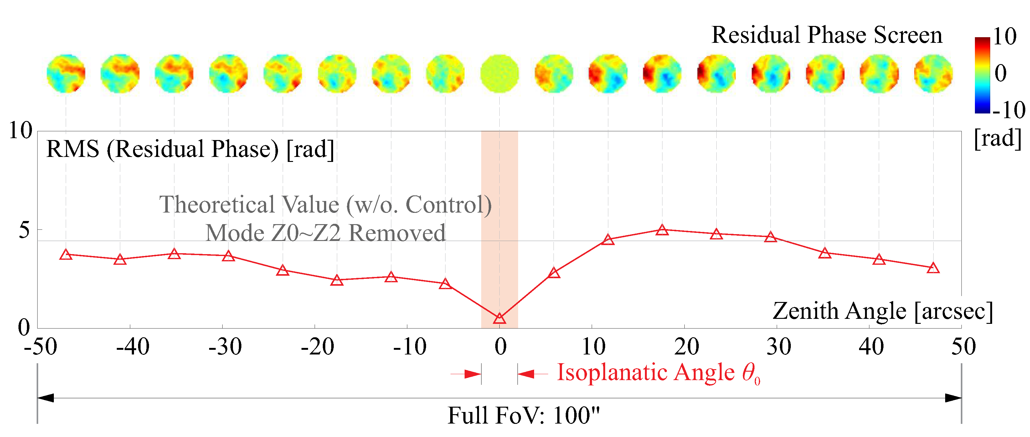
2.1. Modeling Phase Screens by Atmospheric Turbulence

For astronomical observations of distant objects, such as extragalactic stars, the optical wave is typically assumed to be planar until it reaches the outer regions of the Earth’s atmosphere. This assumption is made under the condition that the distance between the source (the star) and the receiver (the telescope) satisfies the far-field condition. The Fried coherence length $r_0$ can be expressed by [5]

$$r_0={\left[0.423k^2\sec \left(\zeta \right){\int }_L{C}_n^2\left(z\right)dz\right]}^{-3/5}$$

(2)

where $k=2\pi /\lambda$ is the wave number, $\zeta$ is the zenith angle, $C_n^2\left(z\right)$ is the structure constant profile of the refractive index along the wave transfer path, and z is the vertical distance. $C_n^2\left(z\right)$ is a measure of turbulence strength. Equation (3) suggests that the distance z should satisfy the criteria of the Fraunhofer far-field condition [20] in order to simplify the spherical wave emitted by a point source to a planar wave. It can be quantified by

$$z\gg \frac{x^2}{\lambda }$$

(3)

where x is the dimension of the observed object. If a target is monitored within a visible range for a wavelength of $\lambda =550$ nm, and a magnification factor of 100 is assumed, the light emitted from an object with an altitude height of 3636 km can be considered as a far-field source, which is beyond the LEO region. The phase screen perturbed by atmospheric turbulence can be modeled under several assumptions. Firstly, the three-dimensional structure of the atmosphere can be approximated as a series of independent two-dimensional layers corresponding to the telescope pupil. These layers introduce disturbances to the optical phase, resulting in image blurring on the camera sensor. The spatial correlation of the aerodynamic quantities, such as the wind velocity and temperature fluctuations, can be simulated using turbulence theories such as the Kolmogorov turbulence model or the von Kármán model [4]. Secondly, the layers causing the phase delay are considered to be frozen screens that are transported by the wind at a certain velocity (i.e., the Taylor assumption; see [21]). This assumption implies that the phase screens remain fixed for a short period of time, allowing for their modeling and simulation. These frozen screens are commonly used to represent the instantaneous phase distortions caused by atmospheric turbulence. In this paper, the von Kármán model is used with an outer scale for the turbulent eddy of 40 m, and the induced wavefront error is projecting on a pupil of $D=1$ m.

Figure 2 illustrates a computed example of modeling the turbulence screens using a three-layer structure, which is commonly used in atmospheric turbulence simulations. The three layers are defined at different heights: $h_G$, $h_M$, and $h_U$, corresponding to the ground, middle, and upper layers of the screens with optical effects, respectively. In the context of observing a small object moving at a height H, the optical path can be visualized as a volume in the shape of a cone, extending from the source to the entrance pupil of the observer. Each cross-sectional plane of this volume, corresponding to each aerodynamic layer, is associated with a phase screen: $P_G$, $P_M$, and $P_U$. These phase screens are driven by wind speeds $v_G$, $v_M$, and $v_U$, respectively, with random directions. It is important to note that the ground layer, typically located at a level of around 100 m, often has the most significant contribution to the phase disturbances among all of the layers [22,23].

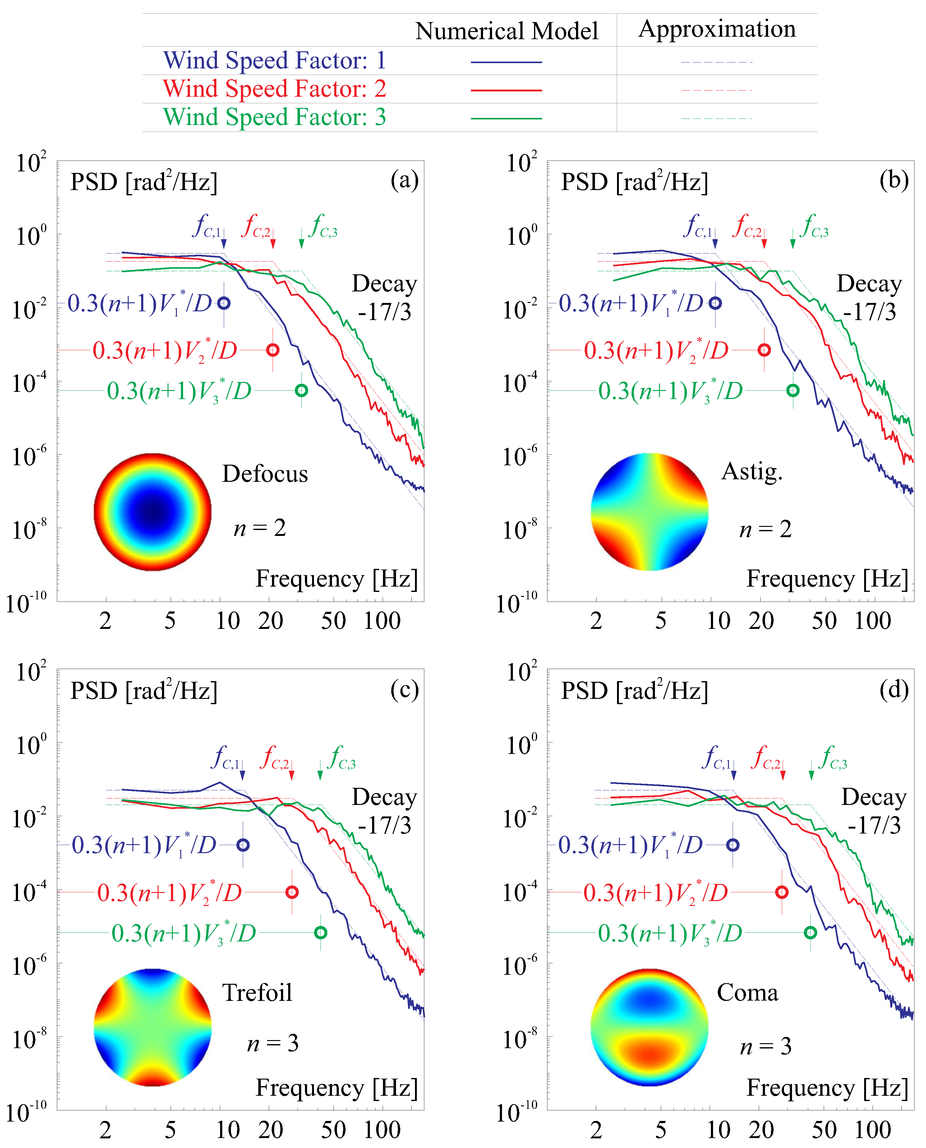
2.1.1. Modal Analysis of a Phase Screen

The final phase screen P projected onto the telescope pupil can be regarded a function of the zenith angle $\zeta$ and time t, denoted as $P=P(\zeta ,t)$. The strength or severity of a phase screen can be quantified using a statistical measure called the Mean Square (MS) value. The MS value provides an estimation of the average magnitude or intensity of the phase error across the screen. According to [6], uncorrected turbulence over an aperture of diameter D results in a residual value of

$${\sigma }_P^2=1.03{\left(\frac{D}{r_0}\right)}^{5/3}$$

(4)

The aberrations of the optical phase P on the pupil, with a diameter of D, can be decomposed into a set of orthogonal and normalized functions $Z_i(\rho ,\theta )$, defined on a unit circle in polar coordinates $(\rho ,\theta )$. These functions are known as Zernike modes [24]. We can categorize the Zernike modes, expressed as $Z_n^m$ with radial order n and azimuth order m, into two types based on their effects on the image formation process: (1) the Tip $Z_1^{-1}$(1) and Tilt $Z_1^1$(2) modes, which are the Zernike modes with $n=1$, and primarily affect the overall alignment and orientation of the image, causing it to tilt or to be blurred in the long exposure process; and (2) other flexible modes, which include all of the Zernike modes other than the Tip and Tilt modes, and they are typically characterized by their ability to induce complex wavefront deformations and aberrations. Some common flexible modes include the Defocus mode $Z_2^0$(4) and the Astigmatism modes $Z_2^{-2}$(3), and $Z_2^2$(5) for $n=2$, as well as the Trefoil modes $Z_3^{-3}$(6) and $Z_3^3$(9), and the Coma modes $Z_3^{-1}$(7) and $Z_3^1$(8) for $n=3$.

Figure 2. (a) Modeling the turbulence screens using a three-layer structure, the phase screens are generated using the parameters listed in

Table 1. Parameters for the generation of the three-layer atmospheric model.

Layer	Height h [km]	Fraction w [%]	Wind Velocity [m/s]
Ground	0.1	70	10
Middle	4	25	15
Upper	10	5	20

, and both FoVs of 100 arcsec and 300 arcsec; (b) demonstration of the effect of the phase screens on image degradation by the disturbing phase screen to the optical phase, the pixel discretization during the image acquisition process, and the field motion. The motion-induced blurring is not plotted as it can be eliminated with a Wiener deblurring filter [25] if the orbital movement within the FoV of the telescope is predictable (see the discussion in Section 3).

Figure 2. (a) Modeling the turbulence screens using a three-layer structure, the phase screens are generated using the parameters listed in Table 1, and both FoVs of 100 arcsec and 300 arcsec; (b) demonstration of the effect of the phase screens on image degradation by the disturbing phase screen to the optical phase, the pixel discretization during the image acquisition process, and the field motion. The motion-induced blurring is not plotted as it can be eliminated with a Wiener deblurring filter [25] if the orbital movement within the FoV of the telescope is predictable (see the discussion in Section 3).

Another important aspect of the atmospheric turbulence screens is the frequential behavior; the coefficients of each Zernike mode are decomposed and a spectral analysis is conducted using the Power Spectral Density (PSD) of the signal of the time series, as shown in Figure 3. Here, we use a simplified model mentioned in [19,26]; the temporal PSDs of the amplitudes of the Zernike polynomials’ expansion of the phase error have been investigated in [21]. For a given radial degree (usually $n>1$), the spectrum ${\mathrm{\Phi }}_Z\left(f\right)$ can be roughly approximated by a constant value ${\mathrm{\Phi }}_{Z,0}$ until the cut-off frequency $f_C$ followed by a decay rate of −17/3. The cut-off frequency depends on the radial order n and the wind velocity according to

$$f_C=0.3(n+1)V^{\ast }/D$$

(5)

In Equation (5), the wind velocity $V^{\ast }$ is computed by the motion of the frozen turbulence screen of one layer; this can be also treated by a weighted quantity if the phase screens are assumed with multiple layers, and the weighting factors of the Fried parameter $r_0$ can be used.

The samples used for computation in Figure 3 come from a zenith sensing of the wavefront for 25,000 independent observations with a sampling frequency of 500 Hz; the wind velocities used in those numerical examples are the parameters of Figure 2, and scaling factors of 2 and 3 are taken into account for the verification of Equation (5). The numerical results show very good agreement with the simplified model. Again, it is worthy to mention that the PSD analyses are usually difficult to conduct if the number of the samples is insufficient. In the spectral analysis, the maximum frequency (the Nyquist frequency) is controlled by the sampling rate; on the other hand, the lower-limit frequency can be estimated by the frequential resolution $f_S/q$, where q is the number of the frame. Thus, if an observation of the rapid moving LEO object is conducted (acquiring very few images), it becomes challenging to capture and analyze high-frequency variations or fine details in the signal, in such cases. The limited number of frames may restrict the ability to resolve specific frequency components or identify critical features in the PSD, such as the corner frequency $f_C$. In this paper, we make an assumption that the coarsely sampled frames hold the same spectral behavior as the PSDs of Figure 3.

2.1.2. Image Formation with a Disturbing Phase

The simulation of image formation is based on the theory of Fourier Optics (FO), as described in references [20,27]. For each frame in the simulation (denoted by the $ith$ frame), the acquired irradiance on the image plane with coordinates u and v is denoted as $I_{N,i}(u,v)$, and it can be simulated from the ground-truth image $I_{G,i}(u,v)$ using the following equation,

$$I_{N,i}(u,v)=F^{-1}\left\{H(f_u,f_v)F\left[I_{G,i}(u,v)\right]\right\}$$

(6)

where $F(·)$ and $F^{-1}(·)$ are Fourier and inverse Fourier operators, respectively. $H(f_u,f_v)$ is the Optical Transfer Function (OTF) defined on the spatial frequencies $f_u$ and $f_v$, which represents the combined effect of the telescope pupil and the atmospheric phase screen. The normalized OTF can be approximated as

$$H(f_u,f_v)=\frac{F\left[\right|h(u,v){|}^2]}{{\int \left|h(u,v)\right|}^{2}dudv}$$

(7)

where $h(u,v)$ is the impulse response, also known as the Point Spread Function (PSF). The OTF is the normalized autocorrelation of the Coherent Transfer Function (CTF), denoted as $H_C$. It can be represented in the form of $H_C=A_T{e}^{jP}$, where $A_T$ is the pupil function for the entrance of telescope optics, and P is the phase distortion due to atmospheric turbulence [28]. It is important to note that the above formulation is most appropriate for an observed object that occupies a small FoV within an isoplanatic region, which is likely suitable for the scenario described in this paper. However, if the observed object becomes larger or moves closer, the effects of anisoplanatism need to be considered, which usually requires significant computational resources [29,30].

Figure 4 presents simulated images of a satellite at LEO orbits with various heights ranging from $H=300$ km to $H=1000$ km. The satellite being tracked is an Earth observation satellite with dimensions of 7 m × 1 m × 1.87 m. The turbulence-induced phase disturbances are superimposed onto the frames with specific zenith angles, and the OTF is computed using Equation (7), considering the pupil size and different atmospheric conditions represented by the Fried length $r_0$, ranging from 1 cm to 10 cm.

The frames are captured sequentially over time, and the formed images are zoomed to focus on the region of interest with various pixel resolutions due to altitude differences. The final images are then normalized and interpolated to enhance clarity and accuracy. In the simulated scenario, it is assumed that a perfect set of telescope optics is utilized within the FoV, for those studies considering the imperfections of the telescope; refer to [31]. At this stage, the assessment of image quality is conducted subjectively, and objective metrics might be employed for further analysis in the following context. The presented images in Figure 4 illustrate that clear observations can be achieved by either creating a closer imaging process or having better atmospheric conditions.

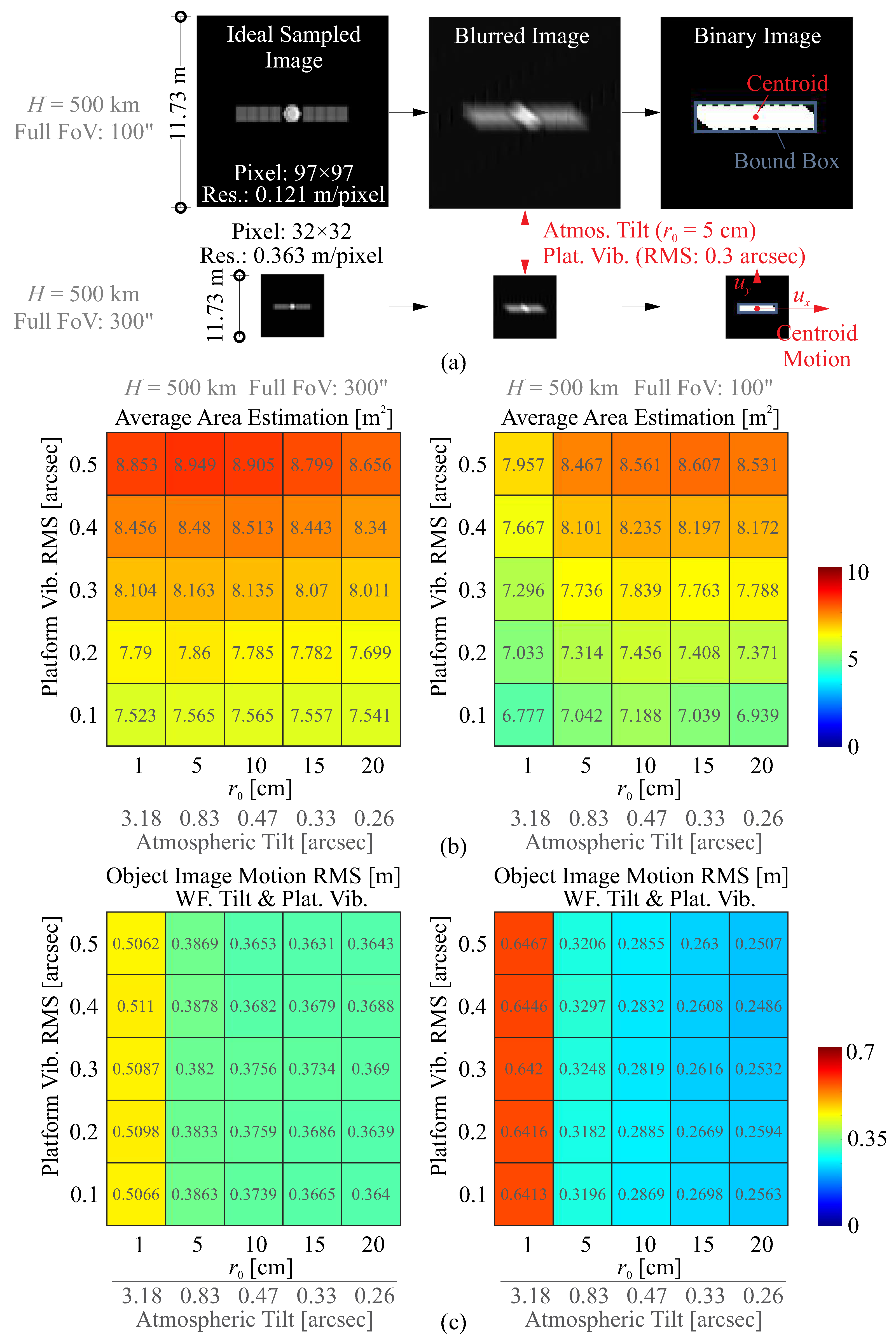
2.2. Image Jitter Due to Optical Tilt

The image jitter in observation can be attributed to two main factors: the incoming tilt wavefront error and the motion or vibration of the observation platform. The tilt error, in particular, is a significant component of the atmospheric wavefront error described in Equation (4), i.e., almost $90\%$ of the MS in a phase screen; the Root Mean Square (RMS) of the two-axis tilt can be estimated using [6]

$${\sigma }_T=\sqrt{0.364{\left(\frac{D}{r_0}\right)}^{5/3}{\left(\frac{\lambda }{D}\right)}^2}$$

(8)

Another significant source of image jitter is the vibration of the telescope structure, which can be attributed to factors such as aerodynamic excitation (e.g., wind in the dome) or seismic excitation. These vibrations can often be mitigated through passive means by optimizing the structural damping or through active measures using a sensor/actuator network [32]. However, even after implementing control measures, there may still be residual motion in the observation field, leading to significant imaging errors. In this study, it is reasonable to request for the pointing error caused by platform vibration to be comparable or smaller in magnitude, specifically in terms of RMS values, compared to the atmospheric tilt. It is worthy to notice that the atmospheric tilt and the platform vibration has distinguished differences in frequential manners.

Figure 5 shows an illustrative plot of both PSDs of the optical tilts caused by the wavefront tilt and the structural vibration. The PSD of the coefficient of the Zernike mode tilt [$Z_1^{-1}$(1) or $Z_1^1$(2)] follows the above discussion with a simplified model as a low pass filter; here, the radial degree for the mode is $n=1$. The PSD has been calibrated according to the value computed from Equation (8). On the other hand, we assume that the residual vibration causes a white tilt spectrum within the Nyquist frequency $f_N$ (one half of the sampling frequency $f_S$); although inaccurate, it can be sufficient to illustrate the idea of Figure 5, and this has been qualitatively proved in [33,34]. In Figure 5, the RMS of the vibration-caused tilt is normalized with the same value as the one of the atmospheric tilt.

In the figure, there are several important frequential quantities marked; the first one is the Greenwood frequency $f_G$ [35], with a mathematical expression of

$$f_G=0.368D^{-1/6}{\lambda }^{-1}{\sec }^{1/2}\left(\zeta \right){\left[{\int }_L{C}_n^2\left(z\right)V^{\ast }dz\right]}^{1/2}$$

(9)

Notice that Equation (9) is only valid for the Zernike mode tilt, which is a more useful approximation, which can be made by $f_G\approx 0.43V^{\ast }/r_0$ [6], with a resulting range of tens to hundreds of Hz. The Greenwood frequency is an indicator of the control bandwidth for the feedback loop design of the telescope system.

The second one is the central frequency $f_W$, computed using the Rice formula

$$f_W=\sqrt{\frac{{\int }_0^{f_{max}}{f}^2\mathrm{\Phi }\left(f\right)df}{{\int }_0^{f_{max}}\mathrm{\Phi }\left(f\right)df}}$$

(10)

This frequency indicates the energy concentration of a signal, and, according to Figure 5, it can be observed clearly that $f_{W,V}\gg f_{W,T}$, showing that the high frequency component within the vibration signal, will significantly deteriorate the imaging process. The differences between these two factors on the image formation will be discussed below.

Figure 6 depicts the impact of optical tilt on image formation, considering both atmospheric tilt represented by the Fried length $r_0$ and platform vibration represented by the RMS value of point errors. Blob analysis is conducted on the acquired images under these conditions. Figure 6a displays images of an orbital object (used in Figure 4) at a height of $H=500$ km, captured with two different FoV sizes: 100 arcsec and 300 arcsec. Zoomed areas of interest are shown for a region spanning 11.73 m, represented by pixel arrays of $97\times 97$ and $32\times 32$ with varying resolutions. To perform the blob analysis, a binarization process is applied to the images, converting them into binary representations. This process enables the extraction and analysis of distinct blob regions. Two parameters are examined in the test: (1) The average area estimate for frames based on the binary pixel information. This parameter provides insights into the size and distribution of the detected blobs; (2) The motion of the observed object, quantified by the RMS values. This parameter indicates the degree of object motion within the captured frames, providing information about the level of image jitter caused by the optical tilt.

Figure 6b presents a table plot showing the average estimated area in the image set for different atmospheric conditions represented by the Fried length $r_0$ and varying levels of vibration, in terms of tilting angle. The corresponding RMS tilt values are also computed and marked based on Equation (8). The obtained areas are significantly influenced by the platform vibration, with a higher level of vibration leading to an overestimate of the area. This is because the vibration introduces motion blur and distortion, causing the observed object to appear larger in the images.

In contrast, Figure 6c demonstrates that the dominant factor affecting the motion of the monitored structure is the atmospheric condition rather than the vibration. This is because the frequency bands at which these factors operate are different. The vibration-induced tilt occurs at a higher frequency band, as illustrated in Figure 5, while the atmospheric tilt typically operates at lower frequencies. When the images are sampled with platform shaking, they are formed in a way similar to long exposure photography, resulting in an expanded and blurred image. Consequently, the final estimated areas can be larger. The motion induced by atmospheric tilt can be sampled clearly, resulting in more apparent movement of the observed object. In addition, comparing the obtained data from the formed images and blob analysis, there exist minor influences by the pixel discretization on those two parameters, a rough pixel meshing (see the example of FoV = 300 arcsec) can usually result in an overestimated area for the moving object.

Figure 7 shows the evaluation of image degradation using an objective metrics, Mean Squared Error (MSE), with a comparison of the reference (ground-truth) imag;, both effects of the atmospheric condition and the pixel discretization of the camera CCD are considered, and the level of vibration is equivalent to a tiling angle on the pupil of 0.1 arcsec in RMS; various Fried lengths ($r_0=1–20$ cm) are considered and different pixel resolutions for certain orbital heights ($H=300$ and 500 km) are examined; the tested object uses the satellite model in Figure 4, the telescope is able to scan a sky coverage of 100 arcsec by a CCD pixel array of $2000\times 2000$. The cases without a disturbing atmospheric phase are also offered. The results indicate a worsening effect the atmospheric aberration quantitatively, and the pixel number also determines the image quality.

3. Scenario Simulation on Observation Opportunities

As mentioned earlier, observing a moving LEO object can indeed be challenging for multiple reasons. Firstly, these orbital structures are typically visible only during a short time period, usually a slot before sunrise and another slot after sunset. This is because LEO objects are often passive in nature and require sufficient sunlight to illuminate them with an adequate order of magnitude of intensity for detection. Secondly, optical telescopes that are designed to capture tiny details of these structures typically have long focal lengths, which results in a narrow FoV. This limitation restricts the number of frames that can be captured with high quality during the observation period. The narrow FoV can make it challenging to track and monitor the LEO object continuously, and it may require precise pointing and tracking mechanisms to maintain the object within the telescope’s FoV, which can be technically difficult to install. These factors, limited observation time, and narrow FoV contribute to the difficulties encountered when observing moving LEO objects and capturing high-quality frames for detailed analysis. In this section, those scenarios are simulated for the count of observation opportunities.

According to the theory of orbital dynamics for a two-body system (Keplerian orbit), the magnitude of the specific angular momentum h for small celestial bodies is

$$h=\omega R^2$$

(11)

where $\omega$ is the angular speed of the orbital object revolving around the Earth, and R is the rotating radius, i.e., $R=R_E+H$, and $R_E$ is the radius of the Earth (assumed as a sphere). Both $\omega$ and R are the functions of the true anomaly ${\theta }_A$. The angular momentum h is a constant for a specific orbit, and if it is elliptic, $h=\sqrt{\mu a(1-e^2)}$, in which $\mu$ is the gravitational parameter of the Earth ($\mu =398600.4418\times {10}^9$ m${}^3$/s${}^2$), a is the length of the semi-major axis, and e is the eccentricity of the orbit, for a elliptic one, $0<e<1$. The rotating radius R can be written as

$$R=\frac{h^2}{\mu }\frac{1}{1+e\cos {\theta }_A}$$

(12)

Combining Equations (11) and (12), we obtain that

$$\omega =\frac{{\mu }^2}{h^3}{(1+e\cos {\theta }_A)}^2$$

(13)

As illustrated in Figure 8a, during the imaging period for an orbital object moving with an angular span of FoV relative to the observer (the telescope), and the angular increment around the Earth is $▵{\theta }_A=H·\mathrm{FoV}/(\mathit{H}+{\mathit{R}}_{\mathit{E}})$ (with respect to the center of the Earth); thus, the fluctuation of the angular speed $▵\omega$ can be roughly estimated using Equation (12), and the computed results are plotted in Figure 8b. In this figure, the variation of the angular speed in terms of the RMS of $▵\omega /\omega$ can be analyzed by considering different eccentricities e of the orbit and varying the FoV of the telescope. The eccentricity of an orbit describes its departure from a perfect circle, with values ranging from 0 (circular orbit) to 1 (highly elliptical orbit). The FoV of the telescope determines the range of angles it can capture during the observation.

By examining the variation of $▵\omega /\omega$ for different eccentricities and FoV sizes, one can estimate the magnitude of the changes in angular speed and assess their impact on the observation of Low Earth Orbit (LEO) objects. For a typical FoV of an optical telescope, the variation in angular speed $\omega$ is relatively small, typically less than $0.05\%$. Even for a survey telescope with a wider FoV, such as a ground telescope with a FoV of $2^{\circ }$, the RMS of $▵\omega /\omega$ is still negligible. When capturing images of LEO objects, if we superimpose the motion of the Earth onto the object’s movement within each captured image, the motion velocities and directions can be considered constant. Additionally, the altitude height of the LEO object can be regarded as constant over a short period of time. These simplifications allow us to treat the object’s motion as relatively steady and predictable, facilitating the observation and analysis of its trajectory and behavior, e.g., the motion caused blurring effect of each captured image will be removed by applying a Wiener deblurring filter, a well known technique used for image restoration and enhancement.

Figure 8c illustrates the maximum number of captured frames, denoted by q, for various FoV sizes during the consecutive imaging process of an orbital target. The range of orbits considered extends from LEO to a MEO with a height approximately equal to that of Global Positioning System (GPS) satellites (approximately 20,200 km). With an image set acquired, the monitored target might be sensed with some small details; an image set refinement strategy will be developed in Section 4.

The scenario simulation presented in Figure 9 provides an analysis of access opportunities for the observation task. To maintain generality, Walker-Delta constellations are used for the simulation [36], which allows for an examination of the access time within a certain period. The Walker-Delta constellation is a solution of layouting the geometric relationship among a huge group of satellites, it can maximize the scanning coverage over Earth and minimize the number of satellites. The layout can be expressed in a format of $i_C:t_C/p_C/P{h}_C$, where $i_C$ is the orbital inclination in degrees, $t_C$ is the total number of the working satellites, $p_C$ is the number of equally spaced geometric planes, and $P{h}_C$ is a phasing difference between satellites in adjacent planes. Three examples are tested as shown on the top of Figure 9, where the layouts are 60: 40/4/1, 60: 80/8/1, and 60: 160/8/1. The simulation considers one ground station with an access to the flying-by satellites, the time slots are one hour before the sunrise and one hour after the sunset for 30 days (one month). The access count is given at the bottom of Figure 9 for various orbital heights.

The results indicate that there are considerable numbers of the access during a certain time period; notice that there are much more numbers of known objects, e.g., artificial satellites with controlled attitudes and unknown structures, such as the asteroids or post-mission satellites at LEO need to be monitored, the latter may no longer be engaged in their original tasks but continue to orbit in space with no control on the attitude. The access count usually increases with the altitudes. Moreover, the numbers of the observation with an elevation angle of ${\theta }_{Elev}>{45}^{\circ }$ are marked, because the observation (the light transmission) with a small elevation angle can be significantly influenced by the aerosol in the atmosphere.

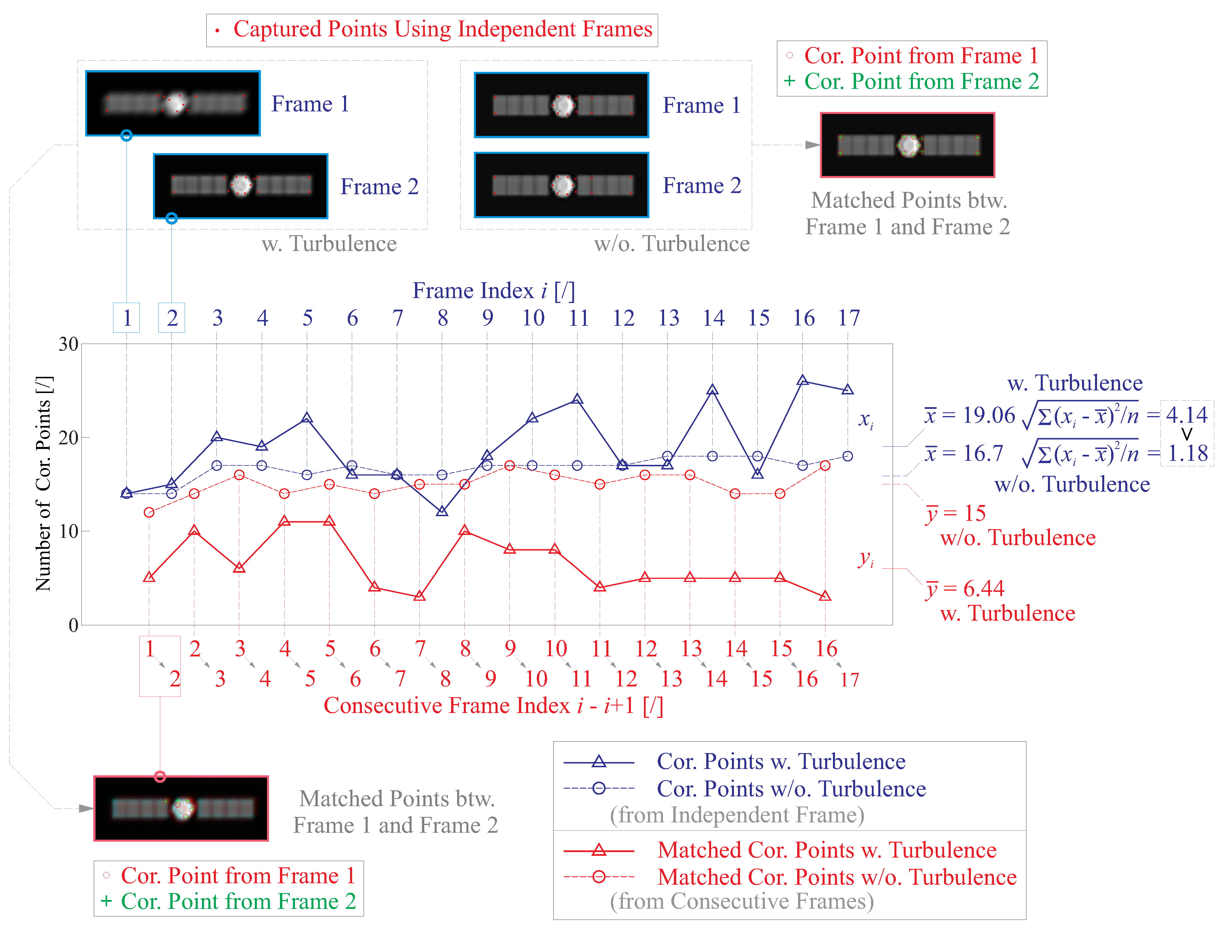
3.1. Tracking on Features of Observed Objects in Consecutive Frames

Figure 10 illustrates the process of detecting corner features for the captured image frames. It involves three steps: (1) a total number of q independent frames are captured and the region of interest (with the monitored object) in each frame is zoomed, all of the zoomed images are normalized and resized (interpolated) with the identical pixel array. (2) The feature nodes within each frame are computed, in this study, we employ the Harris algorithm to search for all the corner nodes upon the variation of the intensity in the image [37,38], a Gaussian filter with an equivalent size of $u_G$ is used to reduce the sensitivities of searching small-scale noisy components; the locations of those points are obtained, and the number of corner points in the $ith$ frame can be denoted by $x_i$. (3) A matching process is conducted between two consecutive images with a threshold distance of $u_M$, with a number of $y_i=g(x_i,x_{i+1})$, where $g(·)$ is the matching operator. The Harris detector is insensitive to overall changes of the gray scale but not scale invariant, this is proper to our application presented in this paper, since the orbital height almost remains unchanged during the imaging process and the received figures can be affected by the scintillation by the atmosphere [39]. Notice that the blurring effect by the atmosphere might influence the detecting process, leading to a possible missing or mistakenly pick-up of features. On the other hand, if we assume the blurring filter for two consecutive images is spatially uncorrelated and the motion of the monitored target is considered within a small region during the sampling period of the telescope camera, the matchable nodes could be recognized to be effective.

In the scenario of Figure 10, the stationary telescope is pointing at the LEO object at an orbital height of $H=500$ km, with a full FoV of 100 arcsec projecting on a camera CCD with a pixel of $2000\times 2000$; the atmosphere condition along the pointing line of sight is $r_0=5$ cm. During the imaging process (the sampling frequency $f_S=500$ Hz), we obtain 17 independent frames with a zooming operation on the region of interest (pixel array dimension: $97\times 97$). In this numerical example, a Gaussian filter with an equivalent size of $u_G=0.5$ m when employing the Harris algorithm, the motion threshold for matching two images is $u_M=0.24$ m. According to Figure 10, if a wavefront contamination of the atmospheric turbulence exists, there will be large fluctuation in the obtained number of capture corner nodes, with a measure of $\sqrt{\sum {(x_i-\overline{x})}^2/q}$, the RMS value of the unbiased errors, which implies that the feature capturing might be suspect if only one frame is considered. This can be relaxed by processing a match between two sampled images, which eliminates corner points outside the acceptable range, and results into a more reliable count of the effective feature nodes. The mean value $\overline{y}$ is significantly reduced for the blurry images with atmospheric turbulence comparing to $\overline{x}$, while the change in the mean value, $\overline{y}-\overline{x}$, can be quite small if the phase disturbance is not involved into the simulation, those tiny changes might be attributed to the small-range motion of the orbital targets or other reasons related to image noises.

Table 2. Statistical results computed using the parameters in Figure 10, various atmospheric conditions are considered ($r_0$ = 1∼20 cm) with two filter window size for the feature detection ($u_G=0.3$ and $0.5$ m).

Equivalent size of the Gaussian filter: $u_G=0.5$ m
$r_0$ [cm]	$\sqrt{\sum {(x_i-\overline{x})}^2/q}$ (w. Turbulence)	$\sqrt{\sum {(x_i-\overline{x})}^2/q}$ (w/o. Turbulence)	$\overline{y}$ (w. Turbulence)	$\overline{y}$ (w/o. Turbulence)
ine 1	5.17	1.18	1.31	15
5	4.14	1.18	6.44	15
10	3.45	1.18	6.88	15
20	2.73	1.18	7.00	15
Equivalent size of the Gaussian filter: $u_G=0.3$ m
1	5.6	1.5	2.68	19.81
5	5.15	1.5	10.88	19.81
10	3.92	1.5	11.06	19.81
20	2.73	1.5	11.44	19.81

reports the statistical results computed using the parameters in Figure 10; various atmospheric conditions are considered ($r_0$ = 1∼20 cm) with two filter window size for the feature detection ($u_G=0.3$ and $0.5$ m). Those results show that an increasing $r_0$ (better atmosphere condition) leads to a smaller variation of the number of Harris corners ($\sqrt{\sum {(x_i-\overline{x})}^2/q}$) derived from an individual image, and also a larger number of recognized corner nodes of matching two consecutive frames ($\overline{y}$). Larger window sizes will reduce the number of detected points, filtering out some small-scale features.

4. Refining for Consecutive Imaging Based on Adaptive Optics and Filtering Strategies

In contrast to conventional passive designs of opto-mechanical configurations for telescope optics, active real-time wavefront error correction has emerged as a promising approach for the ground-based telescopes. This necessitates the use of optical actuators to actively tune the wavefront within a clear pupil. Examples of such actuators include Spatial Light Modulators (SLM), lenses with variable refractive indices, deformable mirrors/reflectors, and metasurfaces. DMs are the most widely employed components in telescope optics for wavefront control. They actively shape the wavefront by mechanically changing their shape using an array of actuators located on the mirror’s backside. In the case of large Earth telescopes, the DMs serve as phase modulators that are conjugated to atmospheric turbulence screens at specific heights within the AO system.

The Single-Conjugated Adaptive Optics (SCAO) system (refer to AO in this paper) is the most commonly used and simplest form of an AO system. It employs a single DM that conjugates with a one-layer atmospheric phase screen. The wavefront error is measured using a S-H sensor, which is illuminated by the NGS, typically the observed target itself. This configuration enables effective compensation of wavefront aberrations within a small FoV, approximately corresponding to the isoplanatic angle ${\theta }_0$ [6]

$${\theta }_0={\left[2.91k^2{\sec }^{8/3}\left(\zeta \right){\int }_H{C}_n^2\left(z\right)z^{5/3}dz\right]}^{-3/5}$$

(14)

If we consider the structure constant of the refraction $C_n^2\left(z\right)$ as a constant along the altitude z, then the isoplanatic angle ${\theta }_0$ can be estimated roughly by substituting Equation (14) into Equation (2), i.e., ${\theta }_0=0.6r_0/L_I$, where $L_I$ is the integral distance of the atmospheric turbulence, and can be computed using the height data of the turbulent screens and corresponding weighting factors. It is important to note that the isoplanatic angle ${\theta }_0$ is typically very small, on the order of magnitude of less than 10 arcsec. Consequently, the AO technique becomes a suitable solution for accurately observing stationary astronomical objects in the night sky, particularly for on-axis observations.

In this paper, our focus is on a specific scenario involving the observation of a moving object in LEO instead of monitoring a stationary object at a distant location. In this context, we adopt the AO system and propose a simple hardware implementation suited for this scenario. Additionally, we develop a post-processing algorithm aimed at refining the captured images obtained through the AO system. This approach allows us to address the unique challenges associated with observing and imaging objects in motion within the LEO environment.

4.1. Wavefront Correctors in the Adaptive Optics (AO) System

The performance of the AO correction is usually evaluated by the Strehl Ratio (SR), denoted as S, which is a measure of the image quality from an optical design perspective of the observation platform. A perfect diffraction-limited telescope has an SR value of 1. It is important to note that computing the SR differs from acquiring the MSE with respect to the ground-truth image. The former takes into account the arrangement of optical surfaces and any potential wavefront error at the terminal focus point for different observation fields, while the latter evaluates images alone, requiring a reference image for comparison.

Both assessment methods provide objective metrics. However, there is no mathematical expression that directly relates these two indicators, as the MSE relies heavily on the reference image. Nevertheless, an acceptable SR value (e.g., S = 0.6–0.8) is typically associated with a low MSE in image representation. The quantitative estimation of the SR value is often linked to the MS phase error ${\sigma }_P^2$, employing approximations such as Marechal’s approximation [7]

$$S=e^{-{\sigma }_P^2}(S>0.1)$$

(15)

The threshold of image acceptability corresponds to $D=r_0$, thus ${\sigma }_P=1$ rad, leading to $S\approx 0.37$ according to Equation (4). A well corrected system has a SR $S\ge 0.8$, corresponding to ${\sigma }_P^2=0.2$ rad${}^2$, that is a wavefront aberration of ${\sigma }_W\approx \lambda /14$. Notice that the effect of a deformable mirror is to introduce a modification of the wavefront twice that of the deformed mirror within the pupil.

The wavefront correctors (i.e., the DMs) are used to minimize the phase error, the number of controlled channels of Degree-of-Freedom (DoF) determines the morphing capability of a DM, the reconstruction of a phase screen can be accomplished zonally or modally. In the modal representation of a phase screen, the Zernike basis is commonly used. The corrector is considered as a modulator for these modes. The number of Zernike modes, denoted as $J_Z$, that need to be perfectly cancelled to achieve a specific Strehl Ratio (SR) for a given value of $D/r_0$, can be obtained by solving the equation [26]

$$S=1-0.29J_Z^{-\frac{\sqrt{3}}{2}}{\left(\frac{D}{r_0}\right)}^{5/3}$$

(16)

The solution $J_Z$ provides the minimum number of DoFs required to achieve a desired image quality. On the other hand, the number of controlled channels or DoFs for zonal correction, which corresponds to the number of actuators of a DM, can be estimated using an empirical formula proposed by [40].

$$S=e^{-\kappa {\left(\frac{D}{r_0}\right)}^{5/3}{N}_A^{-5/6}}$$

(17)

where $N_A$ is the number of the actuators, and $\kappa$ is an empirical constant with a value of $\kappa =0.3$, as suggested by [40]. Comparing the Equations (16) and (17), for the case where $D=1$ m, $r_0=5$ cm at $\lambda =550$ nm, and the desired Strehl Ratio (SR) is $S=0.6$, we obtain $J_Z=220$ by solving Equation (16), and $N_A=211$ by solving Equation (17). If the atmospheric conditions are more relaxed, for instance, with $r_0=10$ cm, the solutions change to $J_Z=58$ and $N_A=53$. These results demonstrate a consistent estimation of the number of DoFs required for the AO control. Moreover, they can be considered equivalent to each other when a large number of DoFs is required.

Figure 11 depicts the phase evolution controlled by an AO system. The scenario involves a LEO object passing through the observation field of a stationary ground telescope. The target is moving at an orbital height of 500 km, and 17 disturbed phase screens are computed for varying pointing directions. The imaging field spans 100 arcsec, and the layered atmospheric turbulence is simulated using the model described in Figure 2. The wavefront sensing is conducted using the phase screen at a zenith angle of $\zeta =0^{\circ }$, allowing for a close match between the real and sensed wavefront within a small range of the field within the isoplanatic angle ${\theta }_0$. The wavefront control is achieved using a DM, which functions as a perfect Zernike polynomial modulator with 180 orders. The residual wavefront change after control is plotted with respect to the pointing angle. Furthermore, the image qualities are evaluated by calculating the MSE compared to a ground-truth image that is normalized (interpolated) using the same pixel mesh within an observation field near the zenith; a $38\%$ reduction can be made within ${\theta }_0$.

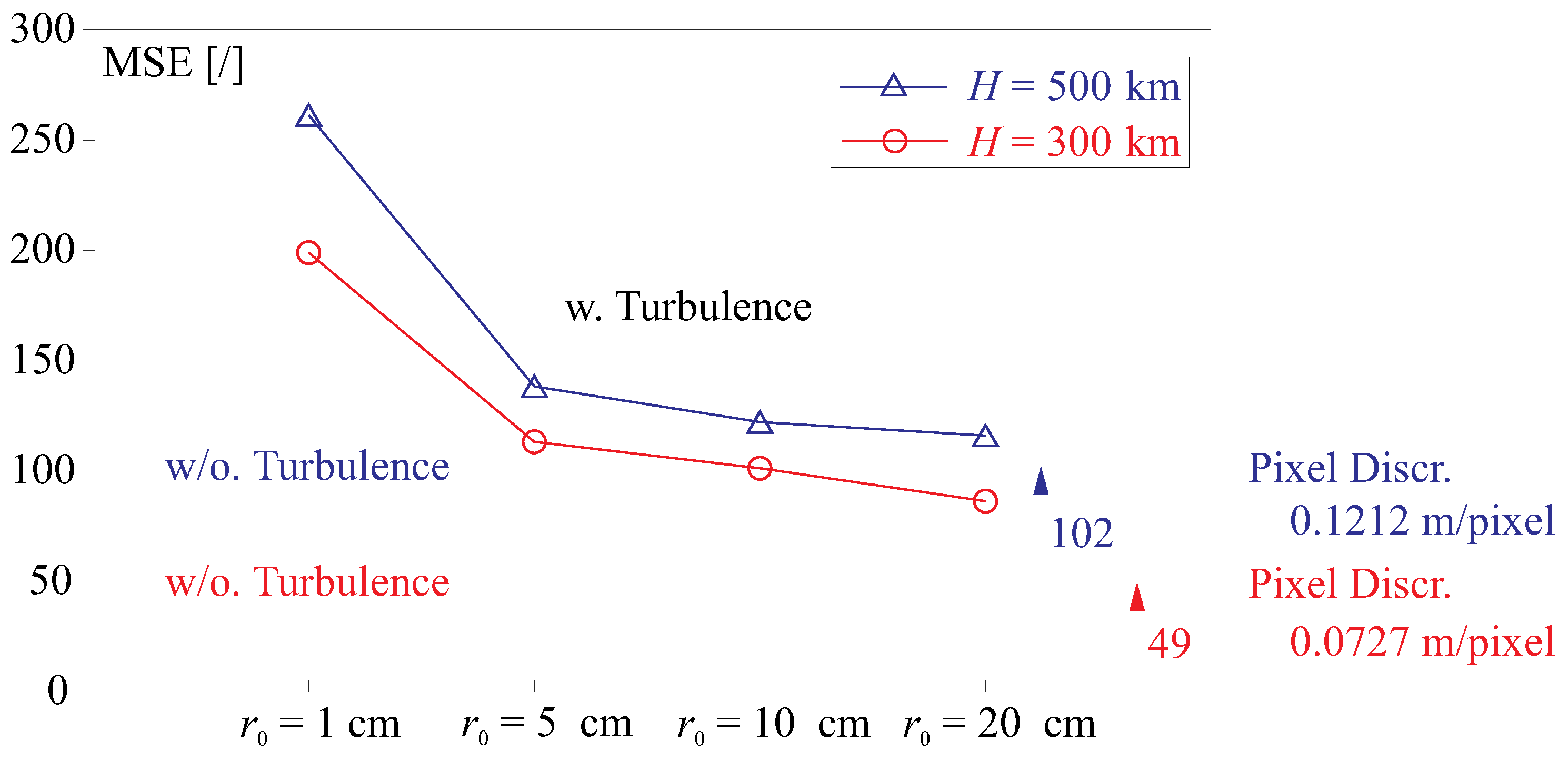
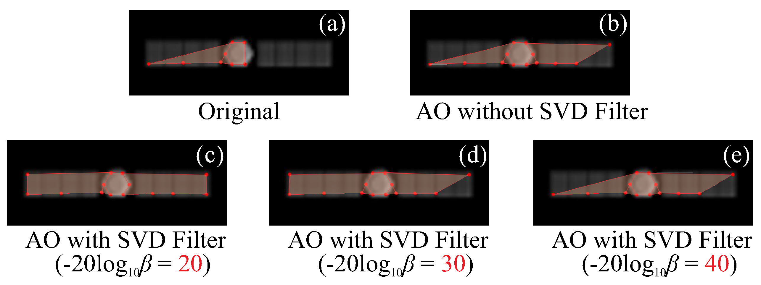
4.2. Refining Strategies of Consecutive Image Set with Singular Value Decomposition Filtering

Despite the improvements achieved through AO correction, there remain several practical challenges: (1) The correction provided by the AO technique is effective within a limited FoV. When an object moves through the telescope’s field, it is challenging to obtain a sufficient number of high-quality images. (2) Tracking feature points typically requires consecutive images, which necessitates a certain level of image quality in neighboring frames. In this study, a refinement strategy can be developed for the acquired image set, incorporating a few AO corrected images as calibrators. This approach aims to address the aforementioned challenges and enhance the overall quality of the image set.

The image set can be organized into two matrices, namely $I_A$ and $I_N$. $I_A$ represents the corrected images, typically with a smaller number of columns denoted by t. In the context of this paper, $t\approx 1$ is considered. It is assumed that the indices of these corrected images are known. The matrix $I_N$ consists of the remaining blurry images, with columns represented by $I_{N,i}$ [$i=1\sim (q-t)$]. To process the set of noisy images, the Singular Value Decomposition (SVD) technique can be applied. The SVD allows for the decomposition of the matrix into its singular values and corresponding singular vectors, providing a means to denoise the images in $I_N$

$$I_N=U\mathrm{\Sigma }{V}^T=\sum _i^{q-t}{\sigma }_i{u}_i{v}_i^T$$

(18)

where the matrix $I_N$ has a dimension of $p\times (q-t)$, p is the total number of the pixels in one image and $q-t$ is the number of the noisy images in the set, usually $p>(q-t)$, U and V are both unitary matrices with columns of $u_i$ and $v_i$, respectively, $\mathrm{\Sigma }$ is a matrix with $q-t$ singular values ${\sigma }_i$ at the diagonal entries. The vectors $u_i$ are the range space of $I_N$, i.e., any image in the set of $I_N$ can be made by a linear combination of $u_i$, the singular values ${\sigma }_i$ represent the weighting for each decomposed mode. A reasonable assumption can be made that the components representing noises are close to white, and most likely to be corresponded to lower weighted singular values. The power of the noise can be quantified by a preset Signal Noise Ratio (SNR) in a sense of signal energies, the modes under this SNR threshold should be filtered out. The SNR is defined by $\mathrm{SNR}=-20{\log }_{10}\beta$, where $\beta$ is the threshold. With this filter, the $q-t$ column of the range space $u_i$ is truncated with r reserved orders, we can use $U_r$ to denote the reserved range space. The AO corrected image $I_A$ can be also decomposed with the basis of $U_r$, i.e., $I_A=U_r{U}_r^T{I}_A+A$, where A is the vector contained in the image $I_A$ and orthogonal to the range of $I_N$. Since we considered the corrected image $I_A$ as a reference, for the calibration of other noise images, A might be an superimposed factor to the noisy image set with a coefficient of $\gamma$ ($\gamma =1$ in the most common situation); in fact, the effectiveness of this method depends on the correction of the wavefront within the isoplanatic angle. The $ith$ noisy image can be refined by

$$I_{NR,i}=U_r{U}_r^T{I}_{N,i}+\gamma A$$

(19)

Figure 12 shows the SVD of the consecutive captured images with atmospheric disturbances for the monitored satellite in Figure 4 at a height of $H=500$ km, they are zoomed to the region of interest. The imaging process spans a FoV of 100 arcsec and the isoplanatic angle is ${\theta }_0\approx 4$ arcsec for $r_0=5$ cm and ${\theta }_0\approx 8$ arcsec for $r_0=10$ cm. One image is captured with a corrected wavefront (the 9^th one among a total of 17 images), and the rest 16 images are blurred. These noisy images are normalized before forming the matrix $I_N$ and the sequence of the singular values is plotted in Figure 12a, a threshold of $\beta =4\times {10}^{-2}$ is illustrated in the figure, i.e., in the example, the modes corresponding to ${\sigma }_1/{\sigma }_k>25$ with respect to the principle component $u_1$ should be eliminated, leading to a filter SNR of 28. In addition, the obtained singular modes with the first 10 orders are also given in Figure 12b, a subjective assessment on those modes can be made that only the first one (the principle component) can be recognized comparing to the ground-truth image. With the refining process of Equation (19), the blurred images might be slight sharpened. This can be beneficial to tracking features for the consecutive images, solving the problem of Figure 10. Figure 13 plots the markable features nodes for different processing methods. In these tests, the Harris corners are obtained with a Gaussian filter of $u_G=0.5$ m for each image, the featured points are recorded with a count of $x_i$ for the refined blurry image $I_{NR,i}$, and $x_A$ for the AO corrected $I_A$. Due to a negligible change in attitude for most of artificial celestial bodies within the short imaging period $T_p$ pointing to the LEO target, in this example, $T_p=0.034$ s, the monitored target can be considered quasi static, i.e., the best qualified image can be obtained from $I_A$, and trackable features might be obtained with following steps: (1) the features are matched between the refined blurry image $I_{NR,i}$ and the reference image $I_A$, which leads to a number of effective corner points $y_i=g(x_i,x_A)$ for these two images. (2) A traversal is conducted for all the refined images with $i=1-q$, and the associated corner nodes are recorded, if we see a featured corner appears at the same location (or within a small region) for more than a preset number $N_{th}$ (e.g., $N_{th}=3$ in this test), this featured corner can be remarked as final recognized nodes.

Figure 13a shows the trackable details of the moving satellite with neither the AO correction nor the SVD filter, part of the satellite bodies and one of the solar panels can be detected, resulting into an insufficient number of markable nodes for further processing of the images. Figure 13b gives the trackable feature nodes with the AO correction, and the SVD filter is deactivated, i.e., $I_{NR,i}=I_{N,i}$ with $\gamma =0$ for each blurry images influenced by the atmosphere or mistakenly corrected by the AO system for an inclined field of observation. Figure 13c–e present processed features marked onto the obtained images, combining both techniques of AO correction and SVD filtering, various values of the SNR threshold are tested ($-20{\log }_{10}\beta =20-40$). The results indicate that with a reasonable range of mode filtering (e.g., $\beta =0.1$), the main features (structural details) can be reserved and the amount of noises might be reduced, see Figure 13c, an almost complete collection of 14 corner nodes can be detected, and most of the structure can be satisfyingly sensed using the above process method. However, if the threshold is set to remove only highest modes, the remaining noises will disturb the feature detection, e.g., $-20{\log }_{10}\beta =40$ shown in Figure 13e. Notice that the feature detection is an automated machine process, and, thus, the resulting frames and markable features can always differ from subjective perspectives; the background images in Figure 13 is for reference and the trackable features are obtained with a sequence of frames.

4.3. Tracking Objects with Attitude Changes

Tracking rapid moving objects with attitude changes is indeed another potential application for this technique. In the context of LEO objects, where the imaging period is typically short, the observable motion of a space structure is often attributed to non-man-made objects such as post-mission satellites or space debris. A rough estimate can be conducted to determine the minimum detectable motion (the in-plane rotation rate) of a unknown space object, using the following parameters. We consider a space object at a height of 500 km moving through an imaging field spanning 300 arcsec, and assume a camera panel pixel array of $2000\times 2000$, which corresponds to a pixel size of 0.3636 m on the image plane. If the structure being observed has a dimension of 3 m, then the minimum detectable in-plane rotation angle is approximately $4.{17}^{\circ }$. During the imaging process, a total of 51 frames with a sampling rate of $f_S=500$ Hz can be obtained with a maximum period of $T_p=0.102$ s. Based on these parameters, the minimum detectable rotation rate can be estimated to be approximately ${\omega }_{S,detect}\approx {70}^{\circ }$/s. It is worth noting that it is usually not possible to observe such a high rotation rate in an artificial structure that is in a working state.

In this paper, we simulate the tracking on an example of space debris with both techniques of AO and SVD filtering as presented in Section 4.2, the example is shown in Figure 14, with an envelope dimensions are around 3.2 m × 1.53 m × 1.27 m, and it spins with a rate of ${\omega }_S$ (${\omega }_S>{\omega }_{S,detect}$).

Figure 15 presents numerical tests of tracking the Harris corner points for a moving object, as shown in Figure 14, orbiting at a height of 500 km. The tests are conducted with various spinning rates ranging from ${\omega }_S={90}^{\circ }$/s to ${\omega }_S={360}^{\circ }$/s. A total of $q=17$ frames are sampled at a rate of $f_S=500$ Hz, with a full FoV of 100 arcsec. The Harris corner features are monitored using the method described in Section 3.1. Two adjacent images are used, and a total of $q-1=16$ matching maps are generated. A threshold based on the maximum detectable distance $u_M$ is applied to create an index matrix for the object in each captured frame. If the Harris corner features can be consecutively detected across the frames, they are considered for tracking and potential reconstruction of the attitude changes of the monitored object in orbit. In these tests, we use the methods of wavefront correction (hardware implementation with the AO technique) and the image processing (software of the SVD filtering) developed in Section 4.2.

Figure 15 shows the trackable Harris corner points for the monitored object spinning at a rate of ${\omega }_S={90}^{\circ }$/s, three scenarios are presented, the first one present the tracking test, without the AO correction and image noise filtering, the atmospheric turbulence blurs all the captured images, and only one point can be tracked with a span of 15 consecutive frames ($2.{52}^{\circ }$ rotated); if both techniques are used, i.e., the AO refinement within the isoplanatic angle and SVD filtering (threshold: $-20{\log }_{10}\beta =30$) are conducted, 2 points can be tracked with the full span of 17 frames. In addition, the reference scenario without the influence of the atmospheric disturbances is considered, and 7 points can be tracked with the full span of 17 consecutive frames. The results of other scenarios are also summarized in

Table 3. Results of numercial tests for trackable Harris corner points of a monitored object spinning rates ranging from ${\omega }_S={90}^{\circ }$/s to ${\omega }_S={360}^{\circ }$/s, with a caputring of 17 frames, the data is presented in a format of $n_{d,P}/L_d$, meaning that $n_{d,P}$ trackable points along a span of $L_d$ consecutive frames.

Spin Rate (${\mathit{\omega }}_{\mathit{S}}$)	Original	AO Correction with SVD Filtering	w/o. Turbulence
${90}^{\circ }$/s	1/15	2/17	7/17
${180}^{\circ }$/s	2/8	2/17	5/17
${360}^{\circ }$/s	1/13	1/17	3/17

, demonstrating the feasibility of tracking with the proposed method. Notice that this can be a promising approach of analyzing the motion and attitude changes of the observed object, if more feature nodes can be detected by increasing pixel of the scanning panel N and the sampling frequency $f_S$. It becomes difficult to track a fast rotating structure in orbit (see Table 3), if the spin rate reduces below the threshold ${\omega }_{S,detect}$, the detection tasks might return to the quasi-static cases in Section 4.2.

5. Conclusions

This paper addresses the challenges associated with ground-based observation of LEO targets and presents practical solutions for observing such objects using on-Earth telescopes. The major challenges, including atmospheric turbulence-induced aberrations, blurring, telescope platform vibrations, and spatial variations caused by target motion, are thoroughly investigated. Additionally, practical factors like the pixel resolution, the FoV, and the focal length of the telescope are also considered.

The paper begins by modeling the optical phase delays using a three-layer structure of atmospheric frozen screens, each driven by independent wind velocities. The resulting phase aberrations approaching the telescope pupil are formed by superimposing these layered screens with appropriate weights. The effect of optical tilts, caused by atmospheric tilts and uncontrollable platform motions, is also examined through blob analysis. In the context of observing a moving LEO object, a scenario simulation is conducted considering practical limitations such as feasible time slots for monitoring and numbers of available frames within the FoV during the imaging process. Walker-Delta constellations with various parameters are tested to estimate access opportunities for the observation task.

The paper proposes a method for detecting LEO targets by identifying Harris corner features in consecutive frames and matching adjacent images, demonstrating the deteriorating impact of atmosphere conditions on the detectable features. A refinement strategy for deblurring the images is proposed, combining the AO hardware implementation and post-processing using SVD filtering of the frame set. The AO correction is considered singly conjugated with the atmospheric layer, effectively compensating for wavefront errors within a small field, with a $38\%$ reduction in Mean Squared Error (MSE) achieved for certain frames within the isoplanatic angle. To overcome this limitation, we introduce a novel technique of utilizing corrected figures (usually a small number of frames) and applying SVD filtering to enhance the quality of observation; with a proper filtering factor ($\beta =0.1$), an almost complete collection of 14 corner nodes can be detected. Finally, the paper explores the observation of unknown objects with uncontrolled attitudes (e.g., space debris) and demonstrates the feasibility of continuously tracking these objects under the influence of atmospheric disturbances using the AO correction with the SVD filtering method.

References

1. Yanagisawa, T.; Kurosaki, H.; Oda, H.; Tagawa, M. Ground-based Optical Observation System for LEO Objects. Adv. Space Res. 2015, 56, 414–420. [Google Scholar] [CrossRef]
2. Lei, X.; Li, Z.; Du, J.; Chen, J.; Sang, J.; Liu, C. Identification of Uncatalogued LEO Space Objects by a Ground-based EO array. Adv. Space Res. 2021, 67, 350–359. [Google Scholar] [CrossRef]
3. Werth, M.; Lucas, J.; Kyono, T.; Mcquaid, I.; Fletcher, J. A Machine Learning Dataset of Synthetic Ground-Based Observations of LEO Satellites. In Proceedings of the IEEE Aerospace Conference, Big Sky, MT, USA, 7–14 March 2020. [Google Scholar]
4. Dainty, J.C. Optical Effects of Atmospheric Turbulence. In Laser Guide Star Adaptive Optics for Astronomy; Springer: Dordrecht, The Netherlands, 2000. [Google Scholar]
5. Fried, D.L. Optical Resolution Through a Randomly Inhomogeneous Medium for Very Long and Very Short Exposures. J. Opt. Soc. Am. 1966, 56, 1372–1379. [Google Scholar] [CrossRef]
6. Tyson, R.K. Priciple of Adaptive Optics; CRC Press: Boca Raton, FL, USA, 2011. [Google Scholar]
7. Roddier, F. Adaptive Optics in Astronomy; Cambridge University Press: Cambridge, UK, 1999. [Google Scholar]
8. Potter, A.E. Ground-based Optical Observations of Orbital Debris: A Review. Adv. Space Res. 1995, 16, 35–45. [Google Scholar] [CrossRef]
9. Sun, R.Y.; Yu, P.P.; Zhang, W. Precise Position Measurement for Resident Space Object with Point Spread Function Modeling. Adv. Space Res. 2022, 70, 2315–2322. [Google Scholar] [CrossRef]
10. Fugate, R.Q.; Ellerbroek, B.L.; Stewart, E.J.; Colucci, D.N.; Ruane, R.E.; Spinhirne, J.M.; Cleis, R.A.; Eager, R. First Observations with the Starfire Optical Range 3.5-meter Telescope. In Proceedings of the 1994 Symposium on Astronomical Telescopes and Instrumentation for the 21st Century, Kailua-Kona, HI, USA, 13–18 March 1994. [Google Scholar]
11. Fugate, R.Q.; Ellerbroek, B.L.; Higgins, C.H.; Jelonek, M.P.; Lange, W.J.; Slavin, A.C.; Wild, W.J.; Winker, D.M.; Wynia, J.M.; Spinhirne, J.M.; et al. Two Generations of Laser-guide-star Adaptive-Optics Experiments at the Starfire Optical Range. J. Opt. Soc. Am. A 1995, 11, 310–324. [Google Scholar] [CrossRef]
12. Fugate, R.Q. Prospects for Benefits to Astronomical Adaptive Optics from US Military Programs. In Proceedings of the Astronomical Telescopes and Instrumentation, Munich, Germany, 27 March–1 April 2000. [Google Scholar]
13. Tyler, D.W.; Prochko, A.E.; Miller, N.A. Adaptive Optics Design for the Advanced Electro-Optical System (AEOS); (Ref: PL-TR-94-1043); Phillips Laboratory: Albuquerque, NM, USA, 1994. [Google Scholar]
14. Dayton, D.; Gonglewski, J.; Restaino, S.; Martin, J.; Phillips, J.; Hartman, M.; Browne, S.; Kervin, P.; Snodgrass, J.; Heimann, N.; et al. Demonstration of New Technology MEMS and Liquid Crystal Adaptive Optics on Bright Astronomical Objects and Satellites. Opt. Express 2002, 10, 1508–1519. [Google Scholar] [CrossRef]
15. Bennet, F.; D’Orgeville, C.; Gao, Y.; Gardhouse, W.; Paulin, N.; Price, I.; Rigaut, F.; Ritchie, I.T.; Smith, C.H.; Uhlendorf, K.; et al. Adaptive Optics for Space Debris Tracking. In Proceedings of the SPIE Astronomical Telescopes + Instrumentation, Montréal, QC, Canada, 22–27 June 2014. [Google Scholar]
16. Copeland, M.; Bennet, F.; Zovaro, A.; Riguat, F.; Piatrou, P.; Korkiakoski, V.; Smith, C. Adaptive Optics for Satellite and Debris Imaging in LEO and GEO. In Proceedings of the Advanced Maui Optical and Space Surveillance Technologies Conference, Maui, HI, USA, 20–23 September 2016. [Google Scholar]
17. Petit, C.; Mugnier, L.; Bonnefois, A.; Conan, J.M.; Fusco, T.; Levraud, N.; Meimon, S.; Michau, V.; Montri, J.; Vedrenne, N.; et al. LEO Satellite Imaging with Adaptive Optics and Marginalized Blind Deconvolution. In Proceedings of the Advanced Maui Optical and Space Surveillance Technologies Conference, Maui, HI, USA, 15–18 September 2020. [Google Scholar]
18. Bastaits, R. Extremely Large Segmented Mirrors: Dynamics, Control and Scale Effects. Ph.D. Thesis, Université Libre de Bruxelles, Brussels, Belgium, 2010. [Google Scholar]
19. Wang, K.; Alaluf, D.; Mokrani, B.; Preumont, A. Control-Structure Interaction in Piezoelectric Deformable Mirrors for Adaptive Optics. Smart Struct. Syst. 2018, 21, 777–791. [Google Scholar]
20. Goodman, J.W. Introduction to Fourier Optics; McGraw-Hill: New York, NY, USA, 1996. [Google Scholar]
21. Conan, J.-M.; Rousset, G.; Madec, P.-Y. Wave-front Temporal Spectra in High Resolution Imaging through Turbulence. J. Opt. Soc. Am. A 1995, 12, 1559–1570. [Google Scholar] [CrossRef]
22. Tokovinin, A. Seeing Improvement with Ground-layer Adaptive Optics. Publ. Astron. Soc. Pac. 2004, 116, 941. [Google Scholar] [CrossRef]
23. Hart, M.; Milton, N.M.; Baranec, C.; Powell, K.; Stalcup, T.; Mccarthy, D.; Kulesa, C.; Bendek, E. A Ground-layer Adaptive Optics System with Multiple Laser Guide Stars. Nature 2010, 466, 727–729. [Google Scholar] [CrossRef] [PubMed]
24. Noll, R.J. Zernike Polynomials and Atmospheric Turbulence. J. Opt. Soc. Am. A 1976, 66, 207–211. [Google Scholar] [CrossRef]
25. Biswas, P.; Sarkar, A.S.; Mynuddin, M. Deblurring Images Using a Wiener Filter. Int. J. Comput. Appl. 2015, 109, 36–38. [Google Scholar] [CrossRef]
26. Wang, K. Piezoelectric Adaptive Mirrors for Ground-based and Space Telescopes. Ph.D. Thesis, Université Libre de Bruxelles, Brussels, Belgium, 2019. [Google Scholar]
27. Voelz, D. Computational Fourier Optics: A MATLAB Tutorial; SPIE Press: Bellingham, WA, USA, 2011. [Google Scholar]
28. Lei, F.; Tiziani, H.J. Atmospheric Influence on Image Quality of Airborne Photographs. Opt. Eng. 1993, 32, 2271–2280. [Google Scholar] [CrossRef]
29. Bos, J.P.; Roggemann, M.C. Technique for Simulating Anisoplanatic Image Formation over Long Horizontal Paths. Opt. Eng. 2012, 51, 101704. [Google Scholar] [CrossRef]
30. Hunt, B.R.; Iler, A.L.; Bailey, C.A.; Rucci, M.A. Synthesis of Atmospheric Turbulence Point Spread Functions by Sparse and Redundant Representations. Opt. Eng. 2018, 57, 024101. [Google Scholar]
31. Schroeder, D.J. Astronomical Optics, 2nd ed.; Academic Press: Cambridge, MA, USA, 2000. [Google Scholar]
32. Tang, T.; Niu, S.; Ma, J.; Qi, B.; Ren, G.; Huang, Y. A Review on Control Methodologies of Disturbance Rejections in Optical Telescope. Opto-Electron. Adv. 2019, 2, 190011. [Google Scholar] [CrossRef]
33. Macmynowski, D.G.; Andersen, T. Wind Buffeting of Large Telescopes. Appl. Opt. 2010, 49, 625–636. [Google Scholar] [CrossRef]
34. Wang, K.; Preumont, A. Field Stabilization Control of the European Extremely Large Telescope under Wind Disturbance. Appl. Opt. 2019, 58, 1174–1184. [Google Scholar] [CrossRef]
35. Tyler, G.A. Bandwidth Considerations for Tracking through Turbulence. J. Opt. Soc. Am. A 1994, 11, 358–367. [Google Scholar] [CrossRef]
36. Walker, J.G. Satellite Constellations. J. Br. Interplanet. Soc. 1984, 37, 559–571. [Google Scholar]
37. Bellavia, F.; Tegolo, D.; Valenti, C. Improving Harris Corner Selection Strategy. IET Comput. Vis. 2011, 5, 87–96. [Google Scholar] [CrossRef]
38. Gueguen, L.; Pesaresi, M. Multi Scale Harris Corner Detector Based nn Differential Morphological Decomposition. Pattern Recognit. Lett. 2011, 32, 1714–1719. [Google Scholar] [CrossRef]
39. Zeng, Q.; Liu, L.; Li, J. Image Registration Method Based On Improved Harris Corner Detector. Chin. Opt. Lett. 2010, 8, 573–576. [Google Scholar] [CrossRef]
40. Madec., P.-Y. Overview of Deformable Mirror Technologies for Adaptive Optics and Astronomy. In Proceedings of the SPIE Astronomical Telescopes and Instrumentation, Amsterdam, The Netherlands, 1–6 July 2012. [Google Scholar]
Figure 1. Comparisons of several limiting factors that control the quality of the acquired images, including the diffraction-limited resolution ( λ / D ), the seeing-limited resolution ( λ / r 0 ), and the pixel-controlled angular resolution ( FoV / N ); the angler sizes of typical orbital objects are also provided.
Remotesensing 15 04718 g001
Figure 3. Temporal PSD of the signal of time series for the Zernike mode coefficients; a zenith observation is assumed. A total 25,000 samples are used for the spectral analysis; the numerical results show very good agreement with the simplified model proposed in [19]. (a) Defoucs; (b) Astigmatism; (c) Trefoil; (d) Coma.
Remotesensing 15 04718 g003
Figure 4. Simulation of the image formation for a space object at LEO; the monitored structure has a dimension of 7 m × 1 m × 1.87 m, the turbulence-induced phase disturbances are superimposed onto the frames with a certain zenith, the formed images are zoomed within the region of interest with various pixel resolutions, and they are post-processed by normalization and interpolation with a mesh array of 1024 × 1024 . (a) Illustration of simulated scenario; (b) H = 300 km; (c) H = 500 km; (d) H = 1000 km.
Remotesensing 15 04718 g004
Figure 5. Illustrative plot of both PSDs of the optical tilts caused by the wavefront tilt and the structural vibration; the PSD of the coefficient of the Zernike mode tilt follows a simplified model as a low pass filter, which starts with a constant at low frequency Φ 0 , and decays with a roll-off rate of −17/3 at the corner frequency f C = 0.3 ( n + 1 ) V / D . Here, the radial degree for the mode is n = 1 . The residual vibration is assumed to cause a white tilt spectrum within the Nyquist frequency f N ; both are normalized to the same RMS values.
Remotesensing 15 04718 g005
Figure 6. Impact of optical tilt on image formation, considering both atmospheric tilt represented by the Fried length r 0 and platform vibration represented by the RMS value of point errors: (a) images of an orbital object at a height of H = 500 km, captured with two different FoV sizes: 100 arcsec and 300 arcsec. Zoomed areas of interest are shown for a region spanning 11.73 m, the blob analysis is performed; (b) table plot showing the average estimated area in the image set for different atmospheric conditions and varying levels of vibration; (c) table plot showing the RMS motion of the target in the image set for different atmospheric conditions and varying levels of vibration.
Remotesensing 15 04718 g006
Figure 7. Image degradation by both effects of the atmospheric condition and the pixel discretization of the camera panel, various Fried lengths ( r 0 = 1∼20 cm) are considered and different pixel resolutions for certain orbital heights ( H = 300 and 500 km) are examined, the tested object uses the satellite model in Figure 4, the telescope is able to scan a sky coverage of 100 arcsec by a panel pixel array of 2000 × 2000 ; the image qualities are measured using Mean Squared Error (MSE) comparing with the ground-truth images.
Remotesensing 15 04718 g007
Figure 8. Scenarios of observing a LEO object and a simple estimation on the orbital dynamics: (a) an illustration on the computation of the angular speed of the orbital object ω with respect to the center of the Earth; (b) the variation of the angular speed in the RMS of ω / ω , various eccentricities e are used with FoV ranging from 100 arcsec (optical telescope) to 2 (survey telescope); (c) the maximum number of captured frames for various FoV sizes during the consecutive imaging process of an orbital target.
Remotesensing 15 04718 g008
Figure 9. Scenario simulation for the analysis of access opportunities for the observation task, Walker-Delta constellations are used for the simulation. Three examples are tested with the layouts of 60: 40/4/1, 60: 80/8/1, and 60: 160/8/1. The simulation considers one ground station with an access to the flying-by satellites, the time slots are one hour before the sunrise and one hour after the sunset for 30 days. The access count is given at the bottom of the figure for various orbital heights, the numbers of the observation with an elevation angle of θ E l e v > 45 are marked.
Remotesensing 15 04718 g009
Figure 10. Detectable corner points by Harris algorithm for the monitored object at an orbital height of H = 500 km, the telescope camera has a full FoV of 100 arcsec, capturing q = 17 independent frames under an atmospheric condition of r 0 = 5 cm. The images are normalized and resized (by interpolation) with a pixel array of 1024 × 1024 , and the corner points are computed with a Gaussian filter having an equivalent size of u G = 0.5 m, and the matching process uses a threshold of u M = 0.24 m. Both scenarios with and without atmospheric turbulence are simulated.
Remotesensing 15 04718 g010
Figure 11. Phase evolution with the control of AO, the scenario considers a monitored object moving by the observation field of a stationary ground telescope, the target is at an orbital height of 500 km and 17 disturbed phase screens are computed corresponding to a vary of pointing directions, the total span of the imaging field is 100 arcsec, the layered atmospheric turbulence is simulated using the model described in Figure 2.
Remotesensing 15 04718 g011
Figure 12. SVD of the noisy image set I N , the images are obtained by a consecutive capturing of the monitored target moving at a height of H = 500 km, with an atmospheric condition of r 0 = 5 cm, 17 images are obtained, in which the 9th image is the one with corrected incoming wavefront. (a) the sequence of the singular values with a threshold of β = 4 × 10 2 for illustration; (b) the singular modes with the first 10 orders corresponding to a descending weighting value of σ i .
Remotesensing 15 04718 g012
Figure 13. Markable features nodes for different processing methods: (a) the trackable details of the moving satellite with neither the AO correction nor the SVD filter, part of the satellite bodies and one of the solar panels can be detected; (b) trackable feature nodes with the AO correction, and the SVD filter is deactivated; (c) trackable feature nodes with a AO correction and a SVD filtering for a threshold of 20 log 10 β = 20 ; (d) the same as (c) for a threshold of 20 log 10 β = 30 ; (e) the same as (c) for a threshold of 20 log 10 β = 40 .
Remotesensing 15 04718 g013
Figure 14. The dimensions of the space debris used in the simulation, the envelope dimensions are around 3.2 m × 1.53 m × 1.27 m, and it spins with a rate of ω S .
Remotesensing 15 04718 g014
Figure 15. Trackable Harris corner points for the monitored object spinning at a rate of ω S = 90 /s, 17 frames are sampled at f S = 500 Hz with a full FoV of 100 arcsec: (a) without AO correction and image noise filtering, the atmospheric turbulence blurs the captured images, and only one point can be tracked with a span of 15 consecutive frames ( 2 . 52 rotated); (b) the degradation on the imaging process has been relaxed by the AO refinement within the isoplanatic angle and SVD filter (threshold: 30); (c) the reference scenario without the influence of the atmospheric disturbances.
Remotesensing 15 04718 g015