River Discharge Inversion Algorithm Based on the Surface Velocity of Microwave Doppler Radar

Abstract

Non-contact methods, which are of great significance to the measurement of river discharge, can not only improve the efficiency of measurement but can also ensure the safety of equipment and personnel. However, owing to their inherent drawbacks such as the requirement of riverbed topography measurements and the difficulty in determining hydrological parameters such as equivalent roughness height, velocity index, etc., there are still challenges for measuring river discharge with high levels of efficiency and accuracy using non-contact methods. To overcome the aforementioned challenges, a new river discharge inversion method is proposed in this paper. In this method, vertical velocities are divided into inner and outer region velocities which can be described by the logarithmic law and the parabolic law, respectively. Applying the river surface velocities collected by microwave Doppler radar and the vertical velocity distributions, the water depths are estimated according to the continuity of the vertical velocities and the shear stresses, and then, the river discharges are obtained by the velocity–area method. The proposed method not only has a simple formula but also comprehensively considers the influence of different hydrological conditions, making it suitable for different river widths and water depths. In this paper, surface velocities collected by microwave Doppler radar on the Yangtze River and the San Joaquin River are used to invert the river discharge, and the results show that for wide–shallow, wide–deep, and narrow–shallow river conditions, the mean percent error ($MPE$) values of the discharges invertedby the proposed method are 3.91%, 3.82%, and 3.6%, respectively; the root mean square error ($RMSE$) values are 4.53%, 5.19%, and 4.81%, respectively; and the maximum percent error ($MaPE$) is less than 15%. The results prove that the proposed method can invert the river discharge with high efficiency and high accuracy under different river widths and water depths without measuring water depth in advance, making it is possible to automatically measure the river discharge in real time.

1. Introduction

River discharge is an important hydrological parameter which is of great theoretical and practical importance in the fields of river hydrology research, water resource management, and flooding control. River discharge values are traditionally obtained using in situ instruments such as current meters [1] and acoustic sensors [2,3]. Nevertheless, measuring discharges requires human operators or instruments placed in contact with the water, making it unreliable, unsafe, or impossible to do so when river surface velocities or waves are high. To manage the problems above, a series of non-contact methods for measuring river discharge have been developed [4,5,6,7,8]. However, all of these non-contact methods still require that the river depth has been previously measured using in situ instruments, which limits their practical application.

In recent years, river discharge estimated from remote sensing derived data has been researched by some scholars, and some progress has been made [9,10,11,12,13,14]. These methods are of great significance to macroscopic flow monitoring. Nevertheless, the spatial and temporal resolutions are not high enough, which makes it challenging to meet the requirements of real-time measurement of river discharge. Microwave Doppler radar, which measures river surface velocities in a non-contact manner under all weather conditions with a high spatiotemporal resolution and high accuracy, has become increasingly mature [15,16,17]. Because of its high performance, microwave Doppler radar has been used in river discharge measurement by some researchers [18,19,20]. To obtain river discharge by microwave Doppler radar, it is essential to derive river depth and mean velocity. C. J. Legleiter et al. [21] obtained river discharge by estimating river depth by applying the relationship between river depth and reflectance of river surface and estimating the mean velocity using the velocity index method. G. Dolcetti et al. [22] obtained river discharge by estimating river depth by applying the dispersion relation for gravity–capillary waves and estimating the mean velocity using the velocity index method. However, the velocity index in these methods is difficult to obtain, the computation of these methods is rather complex, and the results are severely affected by optical conditions, which will limit the application of these methods. Additionally, to apply the above methods in microwave Doppler radar systems, extra optical observation instruments must be installed, resulting in an increase in the complexity and the cost of the radar system.

It would be convenient to estimate river depth and discharge using hydrological methods. D. M. Bjerklie et al. [23] estimated river discharge using Manning’s resistance relationship, and J. A. Simeonov et al. [24] inverted river depth and discharge by applying the steady shallow water equations. However, the former approach requires topography measurements and relies on in situ data to calibrate the unknown coefficients in the empirical relationships, while the latter approach’s computation is rather complex. The vertical distribution of open channel flows can be used to obtain Manning’s resistance coefficient and mean velocity, which can improve the efficiency of river discharge estimation. This has interested researchers for many years, and can be described well by the power law [25], the log law [26,27], the parabola law [28,29], and other forms [30]. With the development of river hydrology research, river vertical velocity distribution is used to invert river depths and discharges using river surface velocities. Lee et al. [31,32] assumed that the vertical velocity distribution of a river could be described by an exponential formula, and then inverted the river discharges using river surface velocities. Li et al. [33] estimated river depths using the power law then obtained the river discharges. Assuming that the mean velocities were 0.85 times that of the river surface velocities, Jin et al. [34] inverted the river discharges, making use of Manning’s equation and the disturbance of open channel flow. However, the parameters such as equivalent roughness height, power exponent, velocity index, etc., in these methods might be too difficult to obtain, making the efficiency and the accuracy of inverting river discharge limited. To address these problems, a new river discharge inversion method is proposed in this paper. In this method, river depths and discharges are inverted on the basis of the surface velocities obtained by microwave Doppler radar and the vertical velocity distributions. Based on the proposed method, river discharges are inverted using the surface velocities obtained by microwave Doppler radar on the Yangtze River and the San Joaquin River, respectively. The inverted river discharges agree well with the results obtained from a nearby hydrological station, proving that the method in this paper could be applied in different river conditions with high efficiency and high accuracy.

The contents of this paper are organized as follows. Section 2 provides the theoretical derivation of the inversion of river discharge. In Section 3, the microwave Doppler radar system is introduced. In Section 4, data collected by the microwave Doppler radar under different river widths and water depths are applied to verify the proposed method. Section 5 analyzes and discusses the results. Finally, Section 6 summarizes the entire text.

2. Inverting Surface Velocity Measurements to Estimate Mean Velocity in the Cross-Section and Discharge

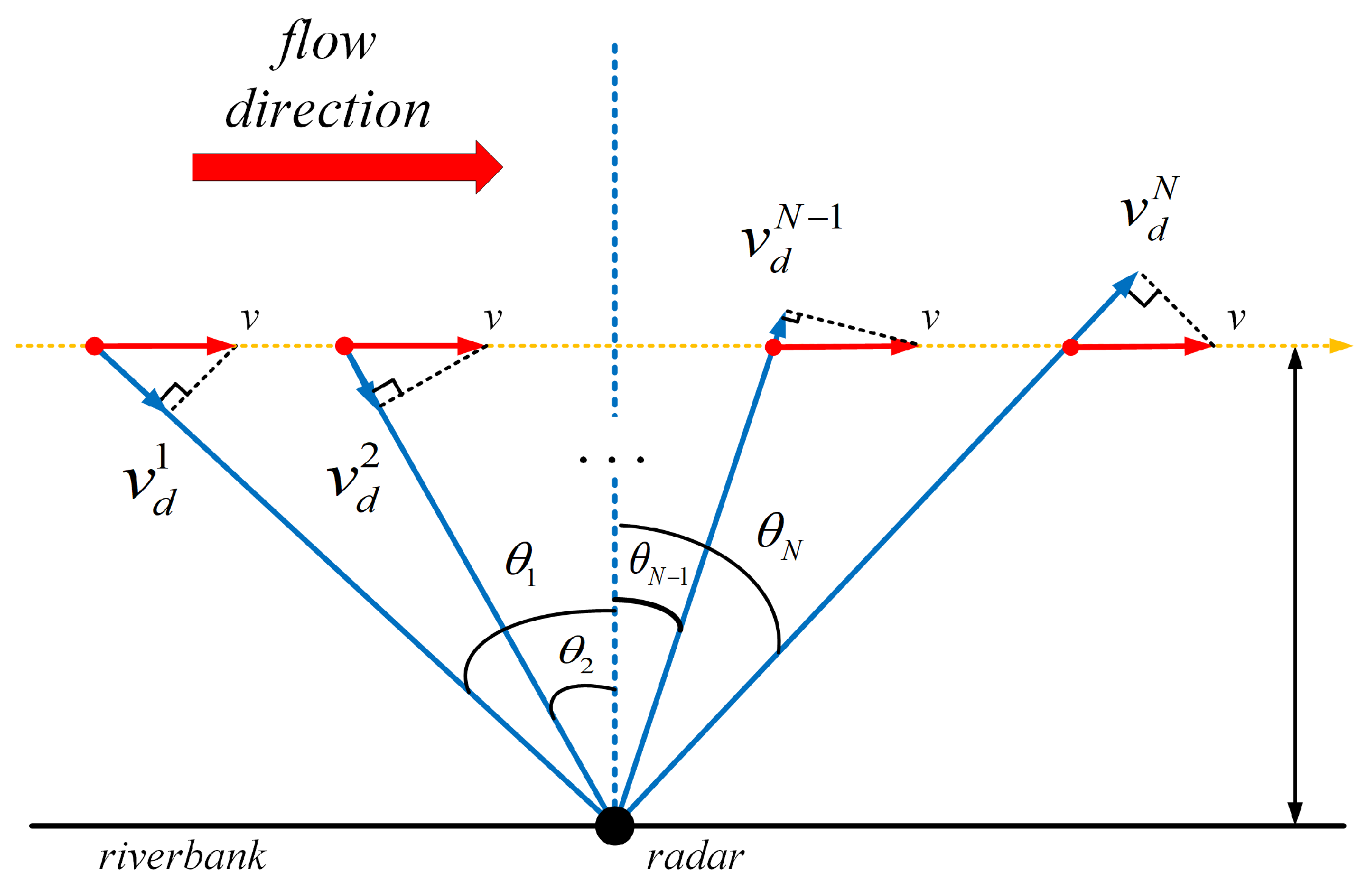
2.1. Measuring River Surface Velocities with Microwave Doppler Radar

The physical phenomenon used to measure river surface velocities with the microwave radars is the Doppler shift, whereby moving objects change the frequency of a signal scattered from them. River surface velocities are measured using the Doppler shift induced in microwave signals backscattered from river surfaces due to advection of the scatterers by the current. When microwaves illuminate rough water surfaces at incidence angles that are not too large or small, they are scattered back to the antenna by short surface waves. This process is known as composite surface scattering in which Bragg-resonant scattering from short surface waves occurs independently from small facets on the water surface that are tilted and advected by larger-scale motions [16,35]. Lengths of those backscattered short waves are well characterized by the Bragg resonance condition

$${\lambda }_b=\frac{\lambda }{2sin{\theta }_0}$$

(1)

where ${\lambda }_b$ is the wavelength of the resonant water wave (the Bragg wave); $\lambda$ and ${\theta }_0$ are the microwave length and the incidence angle, respectively.

As mentioned in the literature [16,35], only Bragg waves traveling radially toward or away from the antenna are effective scatters. Thus, the equation for the Doppler shift, $f_d$, induced in backscattered microwaves due to surface movement with a line-of-sight velocity $v_d$ toward or away from the antenna is

$$f_d=\frac{2v_d}{\lambda }$$

(2)

where $f_d$ is the Doppler shift, which can be estimated from the first moments of the Doppler spectrum $S\left(f\right)$, i.e., $f_d=\frac{\int fS\left(f\right)df}{\int S\left(f\right)df}$.

Then, the river surface velocity $u_s$ is

$$u_s=\frac{v_d\pm v_{w}cos{\theta }_w}{sin\phi }$$

(3)

where $\phi$ is the included angle between antenna azimuth and river flow; $v_w$ is wind-induced surface drift, which is about 3% of the wind speed 10m above the water surface [36] and whose direction is the same as the wind [37]; and ${\theta }_w$ is the included angle between the wind and the antenna azimuth.

For steady and uniform open-channel flows, the flow direction can be considered to be along the river and the velocities of the same streamline are equal; therefore, a monostatic microwave radar can be used to measure the river surface velocities. The river surface velocity of a certain streamline can be calculated by line-of-sight velocities obtained by microwave radar as shown in Figure 1.

Then, the river surface velocity can be expressed as [38]

$$u_s=\frac{1}{N}\sum _{j=1}^N{u}_s^j=\frac{1}{N}\sum _{j=1}^N\frac{v_d^j\pm v_{w}cos{\theta }_w^j}{sin{\theta }_j}$$

(4)

where ${\theta }_j$ is the j-th antenna azimuth, $v_d^j$ is the line-of-sight velocity at angle ${\theta }_j$, and ${\theta }_w^j$ is the included angle between the wind and the angle ${\theta }_j$.

2.2. Calculation of River Discharge

According to the velocity–area method [1], discharge of a river can be expressed as a product of the mean cross-sectional velocity and the cross-sectional area. However, due to the complexity of natural river channel and flow, it is difficult to obtain the mean cross-sectional velocity and the cross-sectional area of a river, making it difficult to calculate river discharge directly. To calculate the discharge, we can uniformly discretize the whole cross-section into subsections in which the water depth is constant, as shown in Figure 2; then, the total river discharge Q can be expressed by the sum of the discharges of the subsections and

$$Q=\sum _{i=1}^M{Q}_i=\sum _{i=1}^M{\overline{U}}_i·S_i$$

(5)

where M is the number of subsections, $Q_i$ is the discharge of the i-th subsection, and ${\overline{U}}_i$ and $S_i$ are the mean cross-sectional velocity and the cross-sectional area of the i-th subsection, respectively.

According to Manning’s equation [34], the mean cross-sectional velocity of the i-th subsection can be expressed as ${\overline{U}}_i=\frac{1}{n}{R}_i^{2/3}{D}_i^{1/2}$. Then, the river discharge can be changed into

$$Q=\sum _{i=1}^M\frac{1}{n}{R}_i^{2/3}{D}_i^{1/2}·S_i$$

(6)

where n is the Manning’s roughness, which can be determined according to factors such as the gravel size of the riverbed, the geological characteristics of the river, etc. [39,40]. To simplify the calculation, we can assume that the gravel size and other factors are the same across the cross-section; so, the Manning’s roughness can be considered to be a constant across the cross-section, $D_i$ is the hydraulic slope of the subsection which equals the slope of riverbed $J_i$ when a flow is uniform [41], and $h_i$ and $R_i$ are the water depth and the hydraulic radius of the subsection which meet $D_i=h_i$. Then, Equation (6) can be rewritten as

$$Q=\frac{W}{M}\sum _{i=1}^M\frac{1}{n}{h}_i^{5/3}{J}_i^{1/2}$$

(7)

where W is the width of river.

2.3. Estimation of Water Depth

As mentioned above, water depth can be estimated by Manning’s equation

$$h_i=n^{3/2}{\overline{U}}_i^{3/2}{J}_i^{-3/4}$$

(8)

For that, an approach widely applied to convert surface velocity $U_{surf}$ to mean velocity is the velocity index, $k_i$, which defined as: $k_i=\frac{{\overline{U}}_i}{U_{suf}}$. Then water depth can be expressed as

$$h_i=k_i^{3/2}{n}^{3/2}{U}_{surf}^{3/2}{J}_i^{-3/4}$$

(9)

The velocity index $k_i$ can be set as 0.85, which is employed in many riverine contexts [18,34]. However, the index is dependent on the shape of vertical velocity profile, which is affected by the factor of river aspect ratio, bed roughness, and so on, making it is difficult to determine a suitable value [42].

Furthermore, mean velocity can be obtained on the basis of vertical velocity distribution, which provides a new way to estimate water depth. According to previous work [26,43,44], the vertical velocity profile can be divided into two parts, as shown in Figure 3; in the inner region, $\frac{z}{h_i}\le 0.2$, the vertical velocity profile follows the logarithmic law [43], and in the outer region, $\frac{z}{h_i}>0.2$, the profile can be described by the log-wake law [44,45] or the parabolic law [28,29]. To make the formula simple and convenient for the subsequent calculation, we choose the latter here to describe the velocities in the outer region.

So, the vertical velocity distribution in the i-th subsection can be expressed as

$$\frac{u_i\left(z\right)}{u_{*}^i}=\left\{\begin{array}{c}\frac{1}{\kappa }ln\left(\frac{z}{z_0^i}\right)=\frac{1}{\kappa }ln\left(\frac{30z}{k_s^i}\right)\begin{array}{cccc}\begin{array}{cc}& \end{array}& & & k_s^i/30\le z\le 0.2h_i\end{array}\\ \frac{u_m^i}{u_{*}^i}-A_i{\left(1-b_i-\frac{z}{h_i}\right)}^2\begin{array}{cccccc}& & & & & 0.2h_i<z\le h_i\end{array}\end{array}\right.$$

(10)

where z is the distance from the actual riverbed, $\kappa =0.4$ is Kalman’s constant, $u_{*}^i=\sqrt{g{h}_i{J}_i}$ is the friction velocity, $z_0^i$ is the virtual riverbed where the velocity is 0 for the natural river $z_0^i=\frac{k_s^i}{30}$ [25], and $k_s^i$ is the equivalent roughness height, whose value is related to the riverbed morphology, flow state, sediment deposition rate and other factors [46,47]. To make Equation (10) meaningful, the vertical velocity should be no less than 0, so, the minimum value for z is the distance between the virtual riverbed and the actual riverbed which is $\frac{k_s^i}{30}$, $u_m^i$ is the maximum vertical velocity, $A_i$ is a constant to be determined by experiments, and $b_i$ represents the velocity deficit coefficient. The values of $u_m^i$, $A_i$, and $b_i$ are related to factors such as the aspect ratio of a river, the flow state and the distance from the riverbank [28].

The mean velocity in the subsection can be expressed as

$$\begin{array}{cc}\hfill & {\overline{U}}_i=\frac{1}{h_i}{\int }_{k_s^i}^{k_s^i+h_i}{u}_i\left(z\right)dz\hfill \\ \hfill & =\frac{0.2u_{*}^i}{\kappa }\left(\left(1+\frac{k_s^i}{6h_i}\right)ln\left(\frac{6h_i}{k_s^i}+1\right)-1\right)\hfill \\ \hfill & +0.8u_m^i-0.8A_i{u}_{*}^i\left({\left(1-b_i\right)}^2-1.2\left(1-b_i\right)+\frac{1.24}{3}\right)\hfill \end{array}$$

(11)

The mean velocity can be calculated by applying Manning’s equation, and Equation (11) can be changed into

$$\begin{array}{cc}\hfill & {\overline{U}}_i=\frac{1}{h_i}{\int }_{k_s^i}^{k_s^i+h_i}{u}_i\left(z\right)dz\hfill \\ \hfill & =\frac{0.2u_{*}^i}{\kappa }\left(\left(1+\frac{k_s^i}{6h_i}\right)ln\left(\frac{6h_i}{k_s^i}+1\right)-1\right)\hfill \\ \hfill & +0.8u_m^i-0.8A_i{u}_{*}^i\left({\left(1-b_i\right)}^2-1.2\left(1-b_i\right)+\frac{1.24}{3}\right)\hfill \\ \hfill & =\frac{1}{n}{h}_i^{2/3}{J}_i^{1/2}\hfill \end{array}$$

(12)

Because water can be considered as a fluid, incompressible, homogeneous, isotropic, and continuous medium, the vertical velocity and velocity gradient distributions are continuous. So, the velocity at the boundary point between the inner and the outer regions is the same. Then,

$$u_i\left(z\right)\left|{}_{z=0.2h_i}\right.=\frac{u_{*}^i}{\kappa }ln\left(\frac{6h_i}{k_s^i}\right)=u_m^i-A_i{u}_{*}^i{\left(0.8-b_i\right)}^2$$

(13)

Combining Equation (12) and Equation (13) we can obtain

$$\left\{\begin{array}{l}{u}_{*}^i\left(\frac{1}{\kappa }ln\left(\frac{6h_i}{k_s^i}\right)\right)=u_m^i-A_i{u}_{*}^i{\left(0.8-b_i\right)}^2\\ \begin{array}{l}\frac{0.2u_{*}^i}{\kappa }\left(\left(1+\frac{k_s^i}{6h_i}\right)ln\left(\frac{6h_i}{k_s^i}+1\right)-1\right)\\ +0.8u_m^i-0.8A_i{u}_{*}^i\left({\left(1-b_i\right)}^2-1.2\left(1-b_i\right)+\frac{1.24}{3}\right)=\frac{1}{n}{h}_i^{2/3}{J}_i^{1/2}\hfill \end{array}\end{array}\right.$$

(14)

From Equation (14), we can infer that the equation is related to the ratio between equivalent roughness height and water depth. Defining parameter $h_k^i=\frac{h_i}{k_s^i}$, Equation (14) can be rewritten as

$$\left\{\begin{array}{l}{u}_{*}^i\left(\frac{1}{\kappa }ln\left(6h_k^i\right)\right)=u_m^i-A_i{u}_{*}^i{\left(0.8-b_i\right)}^2\\ \begin{array}{l}\frac{0.2u_{*}^i}{\kappa }\left(\left(1+\frac{1}{6h_k^i}\right)ln\left(6h_k^i+1\right)-1\right)\\ +0.8u_m^i-0.8A_i{u}_{*}^i\left({\left(1-b_i\right)}^2-1.2\left(1-b_i\right)+\frac{1.24}{3}\right)=\frac{1}{n}{h}_i^{2/3}{J}_i^{1/2}\hfill \end{array}\end{array}\right.$$

(15)

Equation (15) is a set of equations about parameter $h_k^i$, $h_i$, $A_i$, $b_i$, and $u_m^i$. After obtaining the values of $A_i$, $b_i$, and $u_m^i$, the parameter $h_k^i$ and the water depth $h_i$ can be obtained by solving Equation (15), without estimating the equivalent roughness height.

The values of $A_i$, $b_i$, and $u_m^i$ can be obtained using the velocities in the outer region collected by acoustic sensors or other methods. However, it may be difficult or impossible to acquire the vertical velocity distribution when measuring the river discharge, which makes it is necessary to obtain these values according to the vertical velocity distribution formula.

Taking the derivative of vertical velocity profile, we can obtain the vertical velocity gradient distribution as

$$\frac{d{u}_i\left(z\right)}{dz}=\left\{\begin{array}{ccc}\frac{u_{*}^i}{\kappa }\frac{1}{z}\hfill & & k_s^i/30\le z\le 0.2h_i\\ \frac{2A_i{u}_{*}^i}{h_i}\left(1-b_i-\frac{z}{h_i}\right)\hfill & & 0.2h_i<z\le h_i\end{array}\right.$$

(16)

As mentioned above, the vertical velocity gradient distribution is continuous, so

$${\left.\frac{d{u}_i\left(z\right)}{dz}\right|}_{z=0.2h_i}=\frac{u_{*}^i}{\kappa }\frac{1}{0.2h_i}=\frac{2A_i{u}_{*}^i}{h_i}\left(0.8-b_i\right)$$

(17)

and

$$A_i=\frac{5}{2\kappa \left(0.8-b_i\right)}$$

(18)

The relationship between the vertical maximum velocity and the river surface velocity can be obtained from Equation (10),

$$u_m^i=u_s^i+u_{*}^i{A}_i{b}_i^2$$

(19)

where $u_s^i$ is the river surface velocity which is obtained by a microwave Doppler radar.

From Equations (18) and (19), we can infer that the key to obtaining $A_i$, $b_i$, and $u_m^i$ is to obtain the location where the maximum vertical velocity occurs. Researchers have confirmed that due to the presence of secondary currents, the maximum vertical velocity occurs below the river surface [48,49], and whose location is related to the factors such as the aspect ratio of a river, the water depth and the distance from riverbank [50]. When the aspect ratio of a river is greater than five and far away from the riverbank, the maximum vertical velocity can be considered to occur at the river surface [51]; then, $b_i=0$, $A_i=7.81$, and $u_m^i=u_s^i$.

To verify the proposed method in river depth estimation, surface velocities collected by M. C. Lee et al. [31] and R. T. Cheng et al. [49] were used to estimate the water depths, and then, they were compared with the measured results. The scatter plots are shown in Figure 4.

The mean percent errors between the estimated and the measured results were $3.67\%$ and $5.99\%$, respectively, whereas the root mean square error values were $5.02\%$ and $7.44\%$, respectively. Figure 4 shows that the method proposed in this paper can accurately estimate the water depth, which provides a basis for inverting river discharge. Due to a lack of corresponding discharge data, no subsequent discharge comparison will be conducted using the water depth shown in Figure 4a. Based on the corresponding discharge data provided by the literature [49], discharge comparison using the water depth shown in Figure 4b will be performed in Section 5.

A radar may not cover the whole river surface when a river is too wide, which makes it is necessary to estimate the water depth distribution of the whole cross-section using the known results. As mentioned above, the depth and other hydraulic parameters of the river are constant along the river path during radar measuring time, which means that the sidewall of the river is not washed, as shown Figure 5.

Based on the distribution of shear stress on the sidewall, water depth distribution of the river sidewall can be obtained as [43]

$$h^{{}^{\prime }}=hcos\frac{tan\beta }{h}y$$

(20)

where h is the maximum water depth, $\beta$ is the channel sidewall angle at water surface (i.e., the repose angle), and y is the horizontal distance from the maximum water depth position.

To simple the calculation, we assume that the cross-section of the river is U-shaped and symmetrical about the river center line. Then the water depth distribution of the whole cross-section can be estimated by applying the previously estimated water depths and Equation (20). Compensating the cross-section water depth distribution according to the historical data, and then substitute them into Equation (7) to acquire the river discharge.

2.4. Runoff Accuracy Assessment: Error Index

To evaluate the rationality and reliability of this method for river discharge inversion, mean percent error ($MPE$), root mean square error ($RMSE$), and maximum percent error ($MaPE$) are selected as precision evaluation methods. Equations for these methods are defined as follows

$$MPE=\frac{1}{L}\sum _{i=1}^L\frac{\left|Q_e^i-Q_m^i\right|}{Q_m^i}$$

(21)

$$RMSE=\sqrt{\frac{1}{L}\sum _{i=1}^L{\left(\frac{Q_e^i-Q_m^i}{Q_m^i}\right)}^2}$$

(22)

$$MaPE=max\left(\frac{\left|Q_e^i-Q_m^i\right|}{Q_m^i}\right)$$

(23)

where $Q_e$ is the inverted river discharges, $Q_m$ is the measured river discharges, and L is the calculation number.

3. Radar

On the basis of S-band Microwave Ocean Remote Sensor (MORSE) [52], we developed Radio Doppler Velocimetry (RDV) for river hydrological parameter measurement. The radar operates in the S-band at VV-polarization and frequency modulated interrupted continuous wave (FMICW) is used to achieve a high range of resolution, a long detection range, and the time division multiplexing mode for antennas. The operating frequency of radar ranges from 2.75 GHz to 2.95 GHz. The frequency sweeping bandwidth is variable among 10 MHz, 20 MHz, and 30 MHz, which results in a corresponding range resolution of 15 m, 7.5 m, and 5 m, respectively. In addition, a single frequency sweep consists of 256 transmitting pulses with a duty circle near 50%. Therefore, a Doppler dataset consists of 256 echoes.

To obtain the river surface velocities, the RDV is equipped with a waveguide slot array with horizontal and vertical beam widths of 4 degrees and 24 degrees, respectively, and gain of 23 dB. Owing to the adoption of the FMICW, the RDV realizes the sharing of one antenna for transmitting and receiving and reaches a detecting range more than 1 km with a transmitting power of 2.5 Watts. The antenna operates in mechanical scanning model, every antenna covers an area of 4 degrees and requires 10min to collecting data. The radar system is shown in Figure 6. To calculate river surface velocities, data from two antennas are used, therefore, the total time required for detecting river surface velocities is 20 min.

4. Field Experiment and Data Analysis

From March to April 2019, the RDV radar was used to conduct several current measurement experiments at an observation point of Hankou hydrological station located on the north bank of the Yangtze River (114°19′36″E, 30°37′42″N), as shown in Figure 7.

During the experiment, the radar operated at 2.85 GHz with a range resolution of 5 m. The river width at the experimental site was about 1800 m, and the mean depth was about 10 m. The river channel at the site was relatively straight, and changes in the cross-section could be ignored. There were no bridges, dams, or other hydraulic structures in the radar detection area and no heavy rains or floods at the site and no reservoir flood discharges upstream. For these reasons, the flows at the site were constant and uniform during the experiment. Because the aspect ratio at the site was far greater than five, with the river surface detected by the radar far away from the riverbank, it can be considered that the maximum vertical velocity occurred at the water surface. The velocity index method with a velocity index of 0.85 [18] and the method proposed in this paper were used to invert river discharge, respectively, and they were compared with the observation results of the hydrological station, as shown in Figure 8.

It can be seen from Figure 8 that for rivers with wide water surface and shallow water depth, both the proposed method and the velocity index method with a velocity index of 0.85 can be used to accurately estimate the river discharge.

To further study the performance of the proposed method under different hydrological conditions, experiments were carried out at Jiangxin water station (114°24′28″E, 30°39′24.5″N), which is located on the south bank of the Yangtze River from June to July 2022. The locations of the site and the radar are shown in Figure 9.

The radar operating parameters were the same as in 2019. In June, the Yangtze River had a width about 1000 m with a mean water depth about 25 m at the experimental site. Due to the drought in the Yangtze River basin in July, there was a significant decrease in the discharge of the Yangtze River, which made the river width and the mean depth reduce to 920 m and 20 m, respectively.

According to the distributary effect of sandbanks [53], the discharge at the site in June and July accounted for about $60\%$ and $80\%$ of the total discharge, respectively. There was no large flow of tributaries flowing in or out between the site and the hydrological station and no heavy rains during the experimental time. It can be considered that the flow at the experimental site was the same as that at the hydrological station. Then, the velocity index method and the proposed method were used to invert the river discharge, respectively, the results as shown in Figure 10.

It can be seen from Figure 10 that for rivers with wide water surface and deep water depth, the proposed method can accurately invert the discharge. However, due to the changes of the hydrological conditions, there is a significant error in river discharge inversion using the velocity index method, with an index of 0.85.

5. Discussion

The $MPE$, $RMSE$, and $MaPE$ of the proposed method and the velocity index method are calculated for shallow and deep waters as shown in

Table 1. Errors for different river discharge inversion methods.

Depth	Method	MPE (%)	RMSE (%)	MaPE (%)
10 m	The proposed	3.91	4.53	8.7
	velocity index (0.85)	4.32	4.99	10.1
20–25 m	The proposed	3.82	5.19	10.6
	velocity index (0.85)	8.2	9.27	17.3

.

The error distributions between the inverted and the measured results under different water depths are shown in Figure 11 and Figure 12, respectively.

It can be seen from Figure 11 and Figure 12 that the proposed method can invert river discharge with high accuracy under wide shallow and wide deep river conditions. However, as the velocity index is affected by hydraulic parameters such as water depth and riverbed characteristics [42], when the hydraulic parameters change, the velocity index may no longer be equal to 0.85, which will lead to a large bias in inversion using the index of 0.85, as shown in Figure 11 and Figure 12. To accurately invert the river discharge, it is necessary to accurately determine the velocity index, which may be too difficult to perform in practical measurements.

When the river surface is narrow or the water depth is shallow, the maximum vertical velocity may occur below the river surface on the action of the secondary currents. To analyze the performance of the proposed method in such rivers, The data collected by R. T. Cheng et al.’s coherent Doppler radar at X-band (9.36 GHz) on the San Joaquin River from April to May 2002 [49] were used. The width of the river during the experiment was about 70 m, and the mean water depth was about 1.1 m. The locations of the maximum vertical velocities during the experiment are shown in Figure 13.

The river discharges were inverted by the proposed method and the velocity index method whose index is 0.88 [49]. Then, the $MPE$, $RMSE$, and $MaPE$ between the inverted and the measured results are shown in

Table 2. Errors for different discharge inversion methods.

Method	MPE (%)	RMSE (%)	MaPE (%)
The proposed	3.6	4.81	14.03
Velocity index (0.88)	16.73	24.91	70.92

.

Furthermore, the error distribution between the inverted and the measured results with different methods are shown in Figure 14.

From above, we can see that for river conditions with narrow water surface and shallow water depth, due to the complexity of water flow, it is too difficult to accurately determine the velocity index, which leads to the fact that the velocity index method may not accurately invert the discharge. The results show that in rivers with narrow water surface and shallow water depth, although the maximum vertical velocity occurs below the river surface, the discharges can still be accurately inverted using the proposed method. Similarly, the proposed method in this article can also be used to invert the discharges with narrow water surfaces and deep water depths.

As shown above, the proposed method requires a known Manning’s roughness, assumed cross-section geometry, and an energy slope to estimate mean water depth and mean velocity coupled with a measured width to estimate discharge. To accurately invert river discharge, the values of these parameters and the geometry of the cross-section should be carefully selected.

6. Conclusions

Based on the distribution of vertical velocities, this paper proposes a new method for inverting river discharges using surface velocities measured by microwave Doppler radar. The method can efficiently and accurately invert river discharge under different hydrological conditions without measuring river cross-section water depth distribution in advance. This paper analyzes the velocities collected by microwave Doppler radar under different river widths and water depths. The results show that for wide shallow, wide deep, and narrow shallow rivers, the $MPE$ values of the inverted discharge using the proposed method are $3.91\%$, $3.82\%$, and $3.6\%$, respectively; the $RMSE$ values are $4.53\%$, $5.19\%$, and $4.81\%$, respectively; and the $MaPE$ is not more than $15\%$. The results prove that the proposed method in this paper has high accuracy in different river conditions. The experimental results show that the method proposed in this paper can achieve high-accuracy, real-time, and continuous non-contact monitoring of river discharge at anytime and anywhere.

The key to using the proposed method to invert river discharge is to determine the location where the maximum vertical velocity occurs. The experimental results indicate that for rivers with wide water surfaces, assuming the maximum vertical velocity occurs at the surface of the river can achieve accurate results. However, for rivers with narrow water surfaces, due to the secondary currents, the vertical maximum velocity may occur below the river surface. Further research is needed to accurately determine the location of the vertical maximum velocity.

References

1. Herschy, R. The Velocity-area Method. Flow Meas. Instrum. 1993, 4, 7–10. [Google Scholar] [CrossRef]
2. Yorke, T.H.; Oberg, K.A. Measuring River Velocity and Discharge with Acoustic Doppler Profilers. Flow Meas. Instrum. 2002, 13, 191–195. [Google Scholar] [CrossRef]
3. Coz, J.L.; Pierrefeu, G.; Paquier, A. Evaluation of River Discharges Monitored by a Fixed Side-Looking Doppler Profiler. Water Resour. Res. 2008, 44, 1–13. [Google Scholar]
4. Costa, J.E.; Cheng, R.T.; Haeni, F.P.; Melcher, N.; Spicer, K.R.; Hayes, E.; Plant, W.; Hayes, K.; Teague, C.; Barrick, D. Use of Radars to Monitor Stream Discharge by Noncontact Methods. Water Resour. Res. 2006, 42, 1–14. [Google Scholar] [CrossRef]
5. Hong, J.H.; Guo, W.D.; Wang, H.W.; Yeh, P.H. Estimating Discharge in Gravel-Bed River Using Non-Contact Ground-Penetrating and Surface-Velocity Radars. River Res. Appl. 2017, 33, 1177–1190. [Google Scholar] [CrossRef]
6. Fulton, J.W.; Mason, C.A.; Eggleston, J.R.; Nicotra, M.J.; Chiu, C.L.; Henneberg, M.F.; Best, H.R.; Cederberg, J.R.; Holnbeck, S.R.; Lotspeich, R.R.; et al. Near-Field Remote Sensing of Surface Velocity and River Discharge Using Radars and the Probability Concept at 10 U.S. Geological Survey Streamgages. Remote Sens. 2020, 12, 1296. [Google Scholar] [CrossRef]
7. Yang, Y.H.; Wen, B.Y.; Wang, C.J.; Hou, Y. Real-Time and Automatic River Discharge Measurement with UHF Radar. IEEE Geosci. Remote Sens. Lett. 2020, 17, 1851–1855. [Google Scholar] [CrossRef]
8. Chen, Z.Z.; He, Z.Y.; Zhao, C.; Wang, T. Velocity Distribution Inversion Method Based on the RANS Equations Using Microwave Doppler Radar. IEEE Trans. Geosci. Remote Sens. 2022, 60, 5117609. [Google Scholar] [CrossRef]
9. Bjerklie, D.M.; Moller, D.; Smith, L.C.; Dingman, S.L. Estimating Discharge in Rivers Using Remotely Sensed Hydraulic Information. J. Hydrol. 2005, 309, 191–209. [Google Scholar] [CrossRef]
10. Durand, M.; Rodriguez, E.; Alsdorf, D.E.; Trigg, M. Estimating River Depth from Remote Sensing Swath Interferometry Measurements of River Height, Slope, and Width. IEEE J. Sel. Top. Appl. Earth Obs. Remote Sens. 2010, 3, 20–31. [Google Scholar] [CrossRef]
11. Bogning, S.; Frappart, F.; Blarel, F.; Niño, F.; Mahé, G.; Bricquet, J.P.; Seyler, F.; Onguéné, R.; Etamé, J.; Paiz, M.C.; et al. Monitoring Water Levels and Discharges Using Radar Altimetry in an Ungauged River Basin: The Case of the Ogooué. Remote Sens. 2018, 10, 350. [Google Scholar] [CrossRef]
12. Bjerklie, D.M.; Birkett, C.M.; Jones, J.W.; Carabajal, C.; Rover, J.A.; Fulton, J.W.; Garambois, P.A. Satellite Remote Sensing Estimation of River Discharge: Application to the Yukon River Alaska. J. Hydrol. 2018, 561, 1000–1018. [Google Scholar] [CrossRef]
13. Moramarco, T.; Barbetta, S.; Bjerklie, D.M.; Fulton, J.W.; Tarpanelli, A. River Bathymetry Estimate and Discharge Assessment from Remote Sensing. Water Resour. Res. 2019, 55, 6692–6711. [Google Scholar] [CrossRef]
14. Lou, H.; Zhang, Y.; Yang, S.; Wang, X.; Pan, Z.; Luo, Y. A New Method for Long-Term River Discharge Estimation of Small- and Medium-Scale Rivers by Using Multisource Remote Sensing and RSHS: Application and Validation. Remote Sens. 2022, 14, 1798. [Google Scholar] [CrossRef]
15. Plant, W.J.; Keller, W.C.; Hayes, K.; Contreras, R. Measurement of River Surface Currents Using Rough Surface Scattering. In Proceedings of the IEEE Antennas and Propagation Society International Symposium, Washington, DC, USA, 3–8 July 2005. [Google Scholar]
16. Plant, W.J.; Keller, W.C.; Hayes, K. Measurement of River Surface Currents with Coherent Microwave Systems. IEEE Trans. Geosci. Remote Sens. 2005, 43, 1242–1257. [Google Scholar] [CrossRef]
17. Mutschler, M.A.; Scharf, P.A.; Rippl, P.; Gessler, T.; Walter, T.; Waldschmidt, C. River Surface Analysis and Characterization Using FMCW Radar. IEEE J. Sel. Top. Appl. Earth Obs. Remote Sens. 2022, 15, 2493–2502. [Google Scholar] [CrossRef]
18. Costa, J.E.; Spicer, K.R.; Cheng, R.T.; Haeni, F.P.; Melcher, N.B.; Thurman, E.M.; Plant, W.J.; Keller, W.C. Measuring Stream Discharge by Non-Contact Methods: A Proof-of-Concept Experiment. Geophys. Res. Lett. 2000, 27, 553–556. [Google Scholar] [CrossRef]
19. Alimenti, F.; Bonafoni, S.; Gallo, E.; Palazzi, V.; Gatti, R.V.; Mezzanotte, P.; Roselli, L.; Zito, D.; Barbetta, S.; Corradini, C.; et al. Non-contact Measurement of River Surface Velocity and Discharge Estimation with a Low-Cost Doppler Radar Sensor. IEEE Trans. Geosci. Remote Sens. 2020, 58, 5195–5207. [Google Scholar] [CrossRef]
20. Fulton, J.W.; Anderson, I.E.; Chiu, C.L.; Sommer, W.; Adams, J.D.; Moramarco, T.; Bjerklie, D.M.; Fulford, J.M.; Sloan, J.L.; Best, H.R.; et al. QCam: sUAS-based Doppler Radar for Measuring River Discharge. Remote Sens. 2020, 12, 3317. [Google Scholar] [CrossRef]
21. Legleiter, C.J.; Kinzel, P.J.; Nelson, J.M. Remote Measurement of River Discharge Using Thermal Particle Image Velocimetry (PIV) and Various Sources of Bathymetric Information. J. Hydrol. 2017, 554, 490–506. [Google Scholar] [CrossRef]
22. Dolcetti, G.; Hortobágyi, B.; Perks, M.; Tait, S.J.; Dervilis, N. Using Noncontact Measurement of Water Surface Dynamics to Estimate River Discharge. Water Resour. Res. 2022, 58, e2022WR032829. [Google Scholar] [CrossRef]
23. Bjerklie, D.M.; Dingman, S.L.; Vorosmarty, C.J.; Bolster, C.H.; Congalton, R.G. Evaluating the Potential for Measuring River Discharge from Space. J. Hydrol. 2003, 278, 17–38. [Google Scholar] [CrossRef]
24. Simeonov, J.A.; Holland, K.T.; Anderson, S.P. River Discharge and Bathymetry Estimation from Inversion of Surface Currents and Water Surface Elevation Observations. J. Atmos. Ocean. Technol. 2019, 36, 69–86. [Google Scholar] [CrossRef]
25. Chen, C.L. Unified Theory on Power Laws for Flow Resistance. J. Hydraul. Eng. 1991, 117, 371–389. [Google Scholar] [CrossRef]
26. Absi, R. An Ordinary Differential Equation for Velocity Distribution and Dip-Phenomenon in Open Channel Flows. Int. J. Fluid Mech. Res. 2011, 39, 82–89. [Google Scholar] [CrossRef]
27. Snehasis, K.; Koeli, G. An Analytical Model for Velocity Distribution and Dip-Phenomenon in Uniform Open Channel Flows. Int. J. Fluid Mech. Res. 2012, 39, 381–395. [Google Scholar]
28. Sarma, K.V.N.; Lakshminarayana, P.; Rao, N.S.L. Velocity Distribution in Smooth Rectangular Open Channels. J. Hydraul. Eng. 1983, 109, 270–289. [Google Scholar] [CrossRef]
29. Sun, D.P.; Wang, E.P.; Dong, Z.H.; Li, G.Q. Discussion and Application of Velocity Profile in Open Channel with Rectangular Cross-Section. J. Hydrodyn. 2004, 19, 144–151. [Google Scholar]
30. Chiu, C.L.; Chiou, J.D. Structure of 3-D Flow in Rectangular Open Channels. J. Hydraul. Eng. 1986, 112, 1050–1067. [Google Scholar] [CrossRef]
31. Lee, M.C.; Lai, C.J.; Leu, J.M.; Plant, W.J.; Keller, W.C.; Hayes, K. Non-contact Flood Discharge Measurements Using an X-Band Pulse Radar (I) Theory. Flow Meas. Instrum. 2002, 13, 256–270. [Google Scholar] [CrossRef]
32. Lee, M.C.; Leu, J.M.; Lai, C.J.; Plant, W.J.; Keller, W.C.; Hayes, K. Non-Contact Flood Discharge Measurements Using an X-Band Pulse Radar (II) Improvements and Applications. Flow Meas. Instrum. 2002, 13, 271–276. [Google Scholar] [CrossRef]
33. Li, Z.L.; Wang, C.J.; Li, Y.H. Study on the Measurement of the Yangtze River Flow Algorithm Based on UHF Radar. J. Wuhan Univ. (Nat. Sci. Ed.) 2013, 59, 242–244. [Google Scholar]
34. Jin, T.; Liao, Q. Application of Large Scale PIV in River Surface Turbulence Measurements and Water Depth Estimation. Flow Meas. Instrum. 2019, 67, 142–152. [Google Scholar] [CrossRef]
35. Plant, W.J.; Keller, W.C. Evidence of Bragg Scattering in Microwave Doppler Spectra of Sea Return. J. Geophys. Res. Ocean. 1990, 95, 16299–16310. [Google Scholar] [CrossRef]
36. Trizna, D. A Model for Doppler Peak Spectral Shift for Low Grazing Angle Sea Scatter. IEEE J. Ocean. Eng. 1985, 10, 368–375. [Google Scholar] [CrossRef]
37. Polnikov, V.G. Semi-Phenomenological Model for a Wind-Drift Current. Bound.-Layer Meteorol. 2019, 172, 417–433. [Google Scholar] [CrossRef]
38. Yang, Y.H.; Wen, B.C.; Wang, C.J.; Hou, Y. Two-dimensional Velocity Distribution Modeling for Natural River Based on UHF Radar Surface Current. J. Hydrol. 2019, 577, 123930. [Google Scholar] [CrossRef]
39. Lang, S.; Ladson, T.; Anderson, B. A Review of Empirical Equations for Estimating Stream Roughness and Their Application to Four Streams in Victoria. Aust. J. Water Resour. 2004, 8, 69–82. [Google Scholar] [CrossRef]
40. Arcement, G.J.; Schneider, V.R. Guide for Selecting Manning’s Roughness Coefficients for Natural Channels and Floodplains; US Government Printing Office: Washington, DC, USA, 1989.
41. Powell, D.M. Flow Resistance in Gravel-Bed Rivers: Progress in Research. Earth-Sci. Rev. 2014, 136, 301–338. [Google Scholar] [CrossRef]
42. Fujita, M.M.I.; Hauet, A. Large-scale Particle Image Velocimetry for Measurements in Riverine Environments. J. Hydraul. Eng. 2008, 44, 1–14. [Google Scholar]
43. Graf, W.H.; Altinakar, M.S. Fluvial Hydraulics—Flow and Transport Processes in Channels of Simple Geometry; Wiley: New York, NY, USA, 1998. [Google Scholar]
44. Coleman, N. Velocity profiles with Suspended Sediment. J. Hydraul. Res. 1981, 19, 211–229. [Google Scholar] [CrossRef]
45. Guo, J.K. Modified Log-wake-law for Smooth Rectangular Open Channel Flow. J. Hydraul. Res. 2014, 52, 121–128. [Google Scholar] [CrossRef]
46. Camenen, B.; Bayram, A.; Larson, M. Equivalent Roughness Height for Plane Bed Under Steady Flow. J. Hydraul. Eng. 2006, 132, 1146–1158. [Google Scholar] [CrossRef]
47. Camenen, B.; Larson, M.; Bayram, A. Equivalent Roughness Height for Plane Bed Under Oscillatory Flow. Estuar. Coast. Shelf Sci. 2009, 81, 409–422. [Google Scholar] [CrossRef]
48. Sarma, K.V.N.; Prasad, B.V.R.; Sarma, A.K. Detailed Study of Binary Law for Open Channels. J. Hydraul. Eng. 2000, 126, 210–214. [Google Scholar] [CrossRef]
49. Cheng, R.T.; Gartner, J.W.; Mason, R.R.; Costa, J.E.; Plant, W.J.; Spicer, K.R.; Haeni, F.P.; Melcher, N.B.; Keller, W.C.; Hayes, K. Evaluating a Radar-Based, Non-Contact Streamflow Measurement System in the San Joaquin River at Vernalis, California; USGS Open-File Report; USGS: Menlo Park, CA, USA, 2004.
50. Wang, X.K.; Wang, Z.Y.; Li, M.Y. Velocity Profile of Sediment Suspensions and Comparison of Log-Law and Wake-Law. J. Hydraul. Res. 2001, 39, 211–217. [Google Scholar] [CrossRef]
51. Yang, S.Q.; Tan, S.K.; Lim, S.Y. Velocity Distribution and Dip-Phenomenon in Smooth Uniform Open Channel Flows. J. Hydraul. Eng. 2004, 130, 1179–1186. [Google Scholar] [CrossRef]
52. Chen, Z.Z.; Wang, Z.H.; Chen, X.; Zhao, C.; Xie, F.; He, C. S-Band Doppler Wave Radar System. Remote Sens. 2017, 9, 1302. [Google Scholar] [CrossRef]
53. Gao, J. On the Formation of Shoal in River. J. Hydraul. Eng. 1999, 6, 66–70. [Google Scholar]
Figure 1. The configuration of the river and the radar. In the figure, the red arrow represents the direction of the river flow, the orange dashed line is a streamline, the blue solid line represents the antenna azimuth, and the blue dashed line is the normal direction of the riverbank.
Remotesensing 15 04727 g001
Figure 2. The geometry of a river cross-section.
Remotesensing 15 04727 g002
Figure 3. The vertical velocity profile of a uniform flow.
Remotesensing 15 04727 g003
Figure 4. Scatter plots of measured and estimated water depths. (a) Comparison with the water depth collected by M. C. Lee et al. [31], (b) comparison with the results collected by R. T. Cheng et al. [49].
Remotesensing 15 04727 g004
Figure 5. The geometry of a river sidewall.
Remotesensing 15 04727 g005
Figure 6. The configration of the RDV.
Remotesensing 15 04727 g006
Figure 7. The configuration of field experiment and radar in 2019. In the figure, the red dot indicates the radar installation location, the green line indicates the radar reference line parallel to the river bank, the orange line indicates the normal of the river bank, and the blue arrow indicates the surface flow direction of the Yangtze River.
Remotesensing 15 04727 g007
Figure 8. Comparison of different methods for inverting river discharge and measured results. In the figure, the blue line represents the measured results, the red line represents the inversion results using the proposed method, and the green line represents the inversion results using the velocity index method.
Remotesensing 15 04727 g008
Figure 9. The configuration of field experiment and radar in 2022. In the figure, the red dot indicates the radar installation location, the green line indicates the radar reference line parallel to the river bank, the orange line indicates the normal of the river bank, and the blue arrow indicates the surface flow direction of the Yangtze River.
Remotesensing 15 04727 g009
Figure 10. Comparison of different methods for inverting discharge and the measured results. In the figure, the blue line represents the measured results of the hydrological station, the red line represents the inversion results using the proposed method, and the green line is the inversion results using the velocity index method.
Remotesensing 15 04727 g010
Figure 11. Error distribution of the river discharge when the mean water depth is 10 m. (a) The error distribution of the river discharge inverted by the proposed method, (b) the error distribution of the river discharge inverted by the velocity index method.
Remotesensing 15 04727 g011
Figure 12. Error distribution of the river discharge when the mean water depth lies between 20 m and 25 m. (a) The error distribution of the river discharge inverted by the proposed method, (b) the error distribution of the river discharge inverted by the velocity index method.
Remotesensing 15 04727 g012
Figure 13. The locations of the maximum vertical velocities.
Remotesensing 15 04727 g013
Figure 14. Error distribution of the river discharge with different methods. (a) The error distribution of the river discharge inverted by the proposed method, (b) the error distribution of the river discharge inverted by the velocity index method.
Remotesensing 15 04727 g014