


Evaluation of Satellite-Derived Precipitation Products for Streamflow Simulation of a Mountainous Himalayan Watershed: A Study of Myagdi Khola in Kali Gandaki Basin, Nepal


Abstract
:
1. Introduction
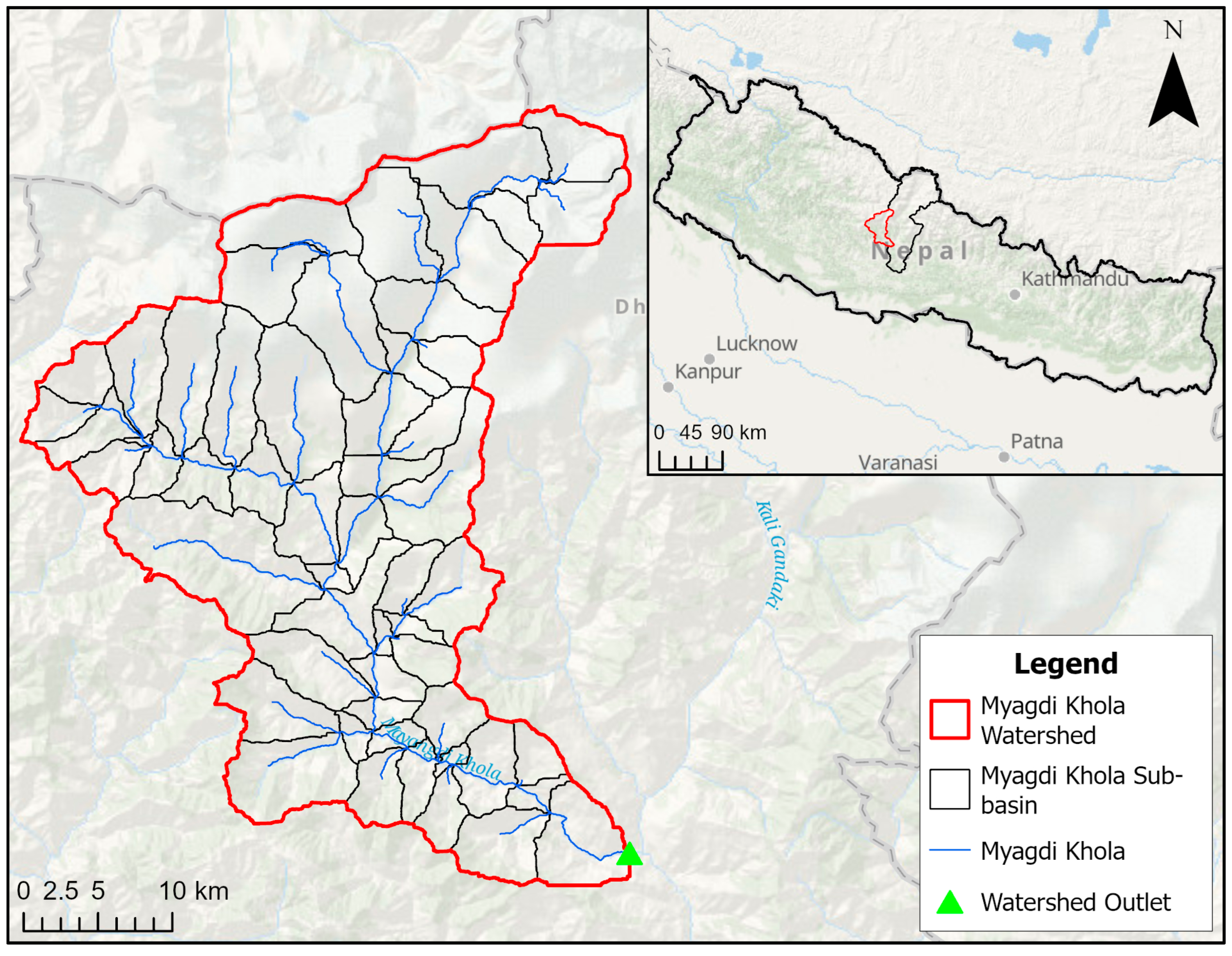
2. Study Area
3. Materials and Methods
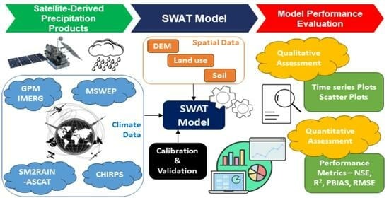
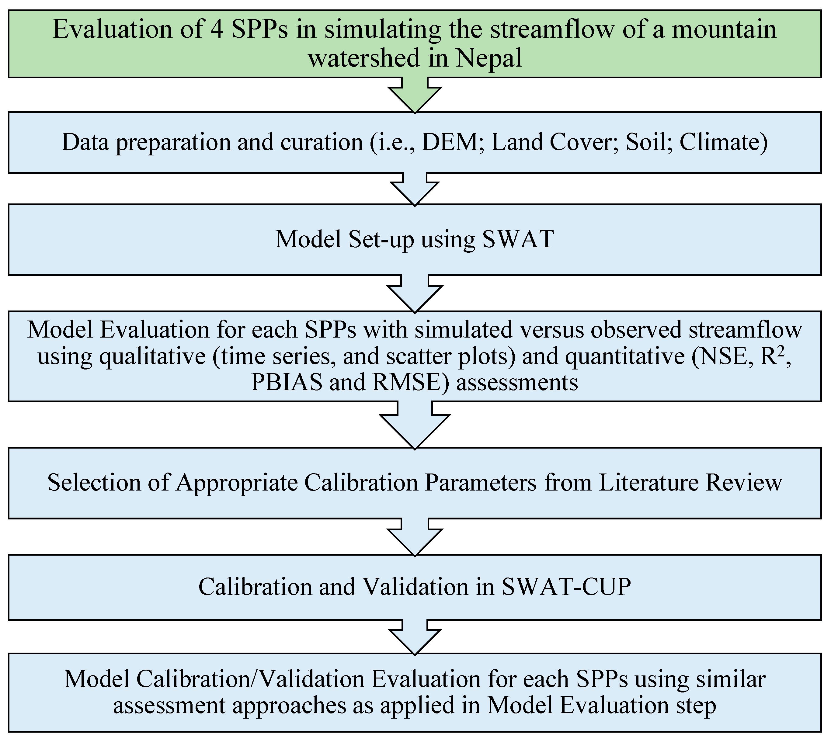
3.1. Methodology
3.2. In Situ Data
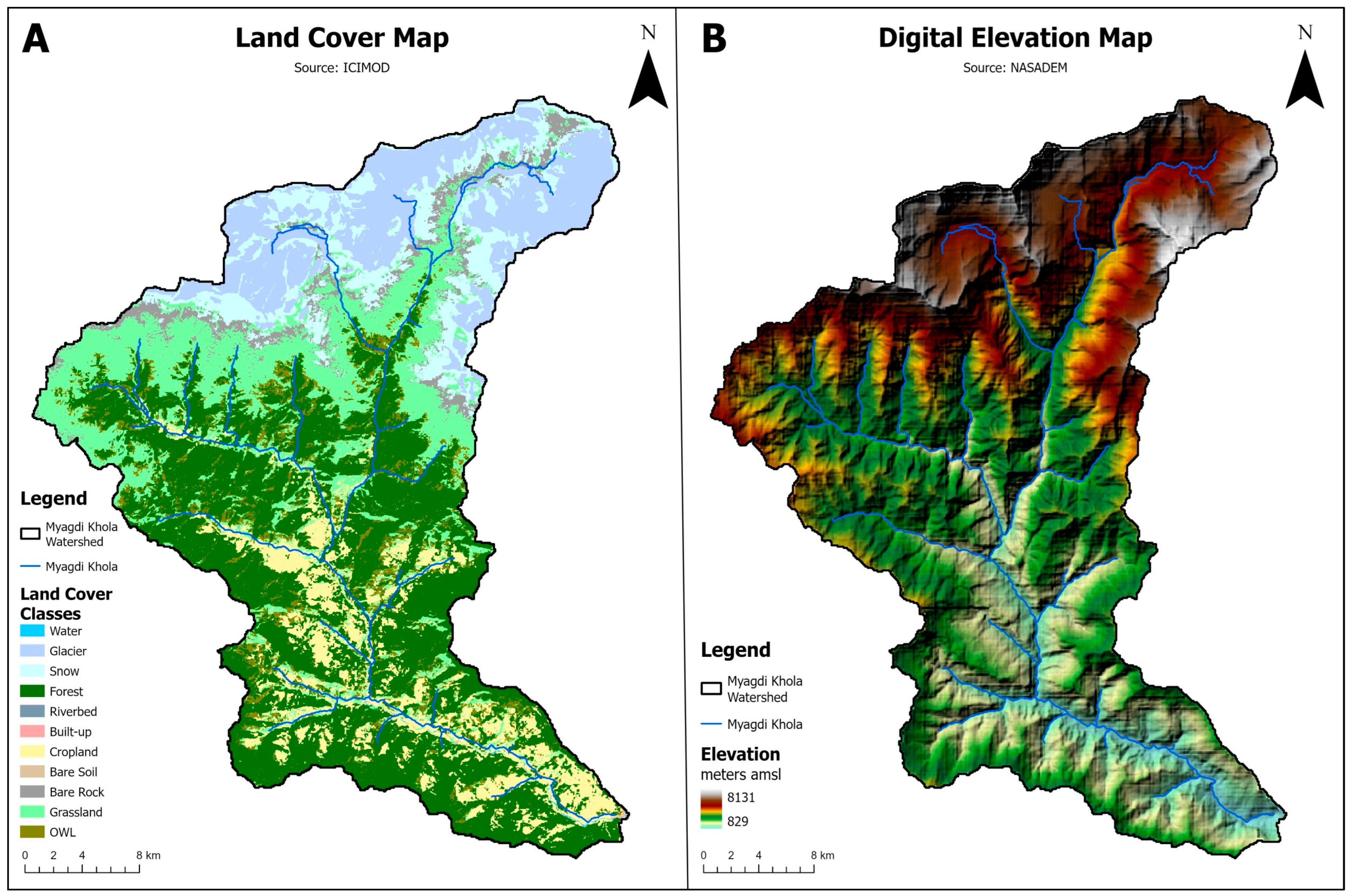
3.3. Spatial Data for SWAT
3.4. Satellite-Derived Precipitation Products
3.4.1. GPM IMERGF
3.4.2. MSWEP
3.4.3. SM2RAIN-ASCAT
3.4.4. CHIRPS
3.4.5. SWAT Model
3.5. Evaluation Metrics
4. Results
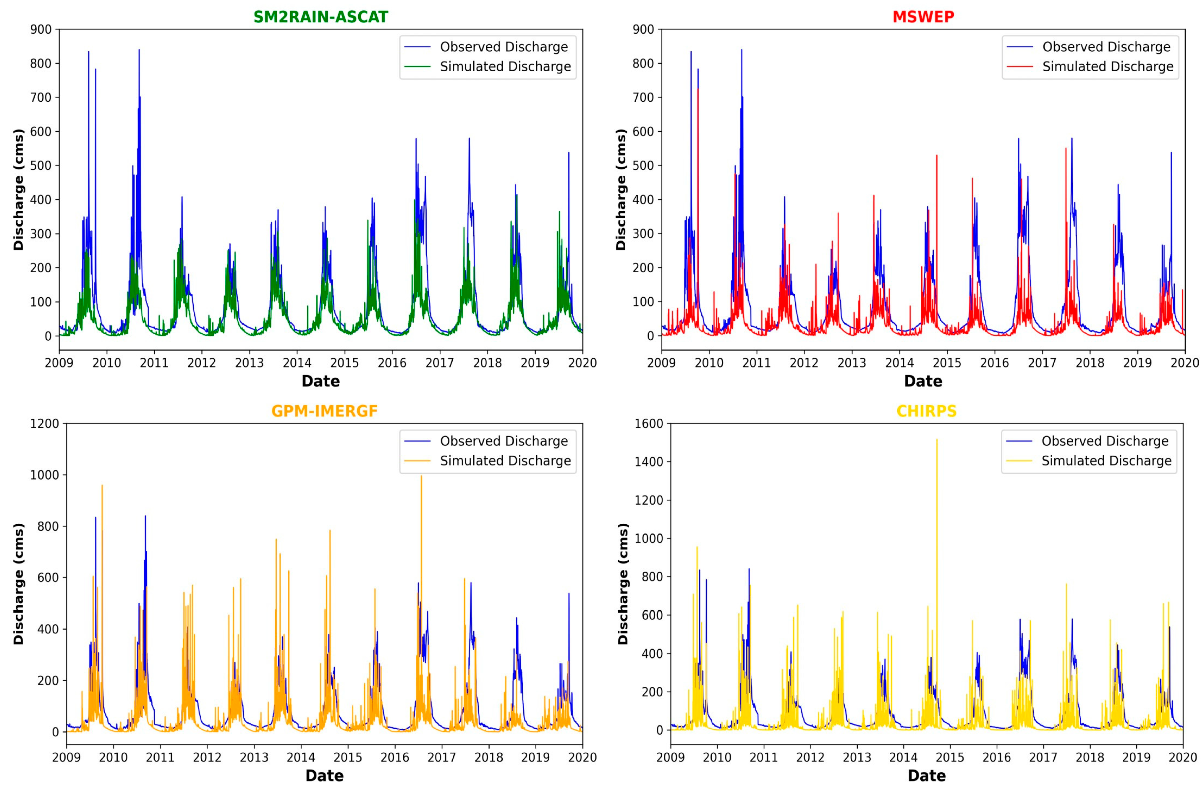
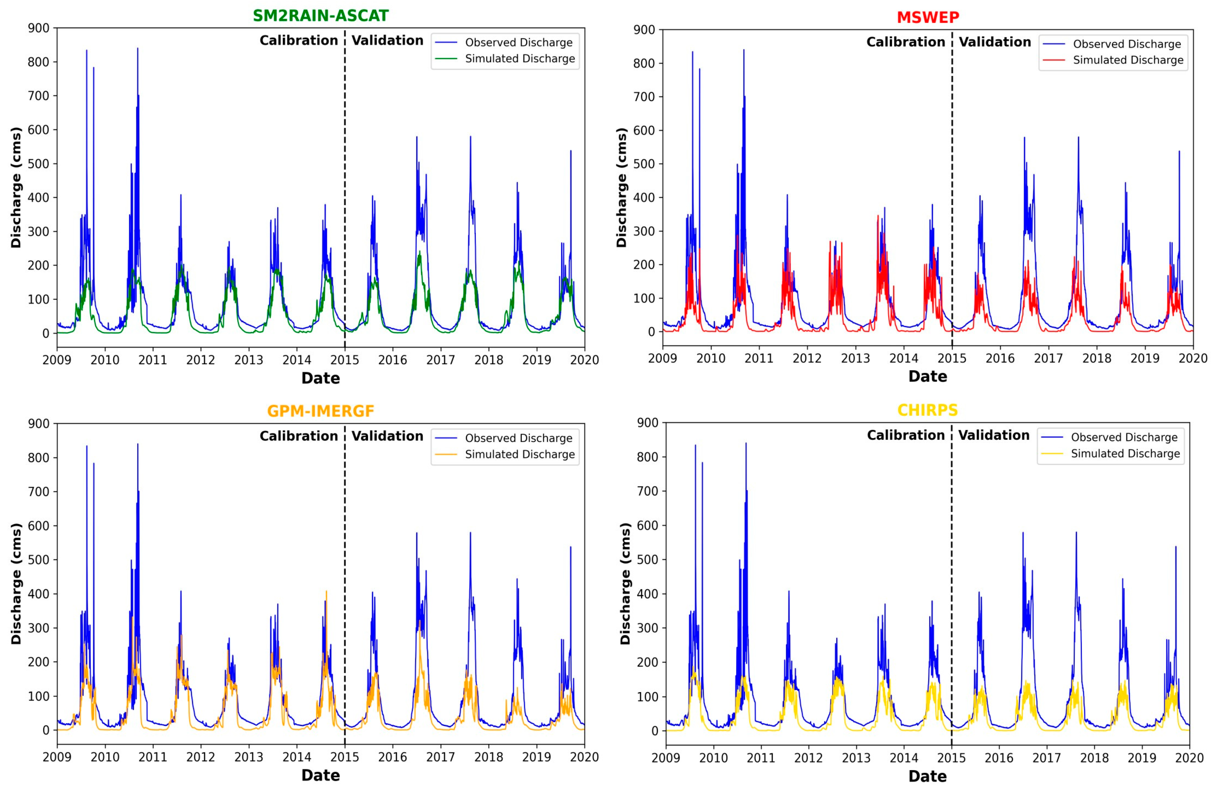
4.1. Qualitative Assessment
4.1.1. Model Evaluation Results
4.1.2. Streamflow Evaluation
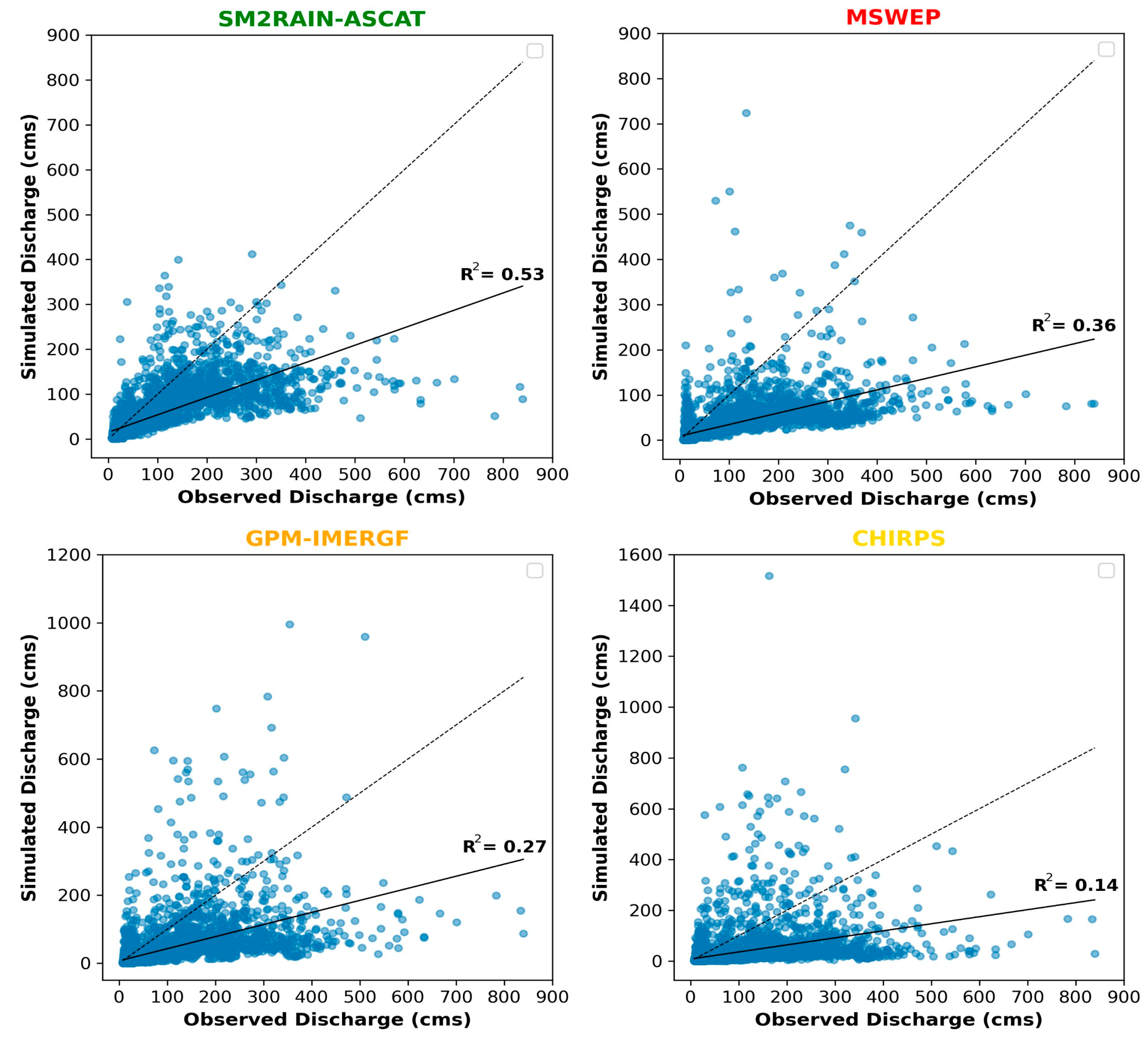
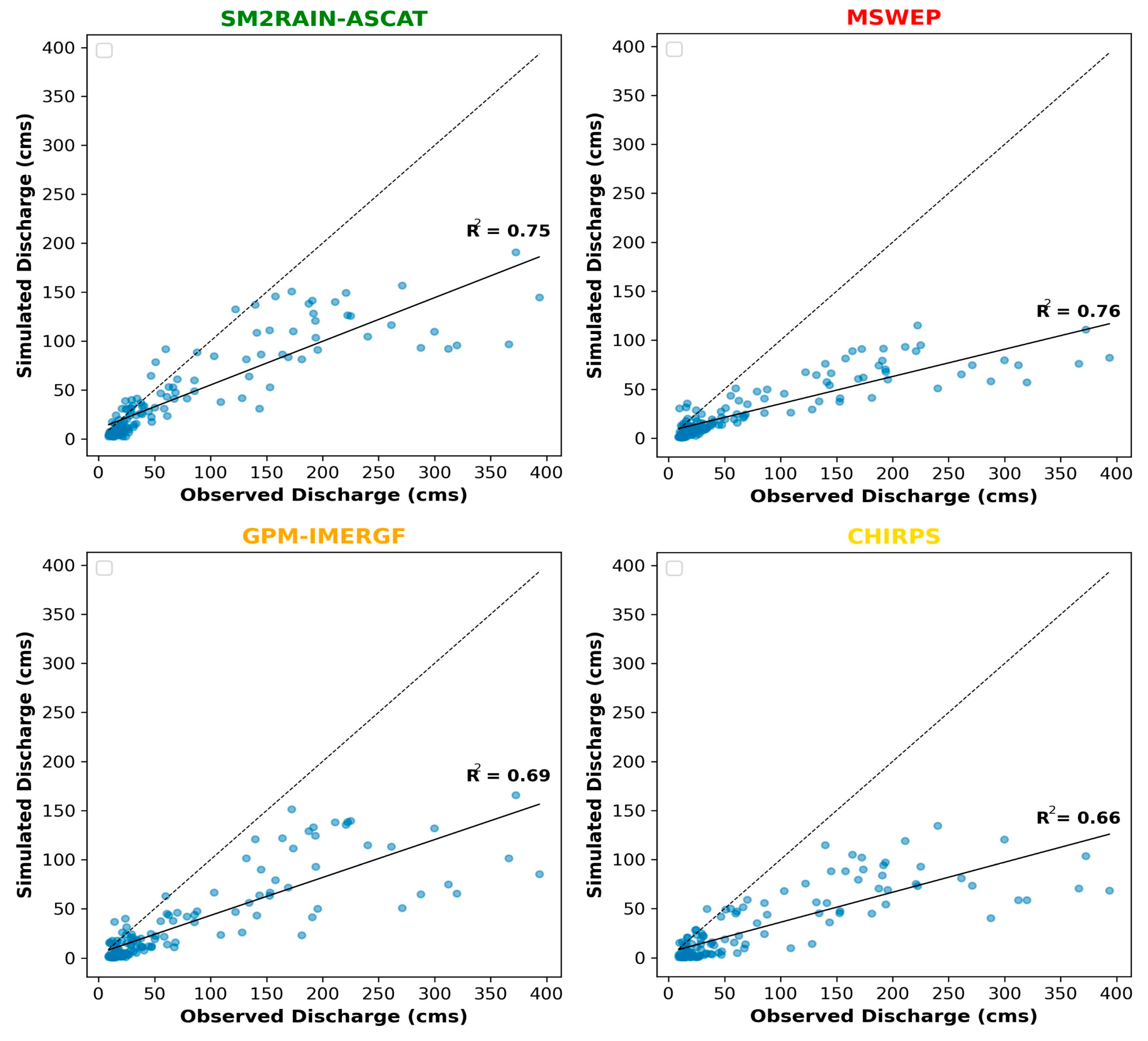
4.2. Quantitative Assessment
5. Discussion
6. Conclusions
- (1)
- The hydrological modeling approach using SPPs effectively predicts streamflow in mountainous watersheds with limited or no observed precipitation data. These products can be used to study hydrological processes in ungauged mountainous watersheds, albeit with some limitations.
- (2)
- Four finer-resolution SPPs were assessed, and SM2RAIN-ASCAT exhibited the best overall performance among other SPPs, followed closely by the GPM IMERGF in simulating streamflow more accurately when compared with observed streamflow at the outlet of the watershed.
- (3)
- Monthly streamflow simulations driven by SPPs outperformed daily streamflow simulations, and gauge-corrected satellite precipitation products fed into the model outperformed in simulating discharge estimates in the watershed. The study found that gauge-corrected SPPs can effectively simulate discharge in Himalayan watersheds, even with limited ground truth data.
- (4)
- Although the performance metrics did not show promising results as anticipated even after the extensive calibration process, they were within satisfactory to good performance levels.
Supplementary Materials
Author Contributions
Funding
Data Availability Statement
Acknowledgments
Conflicts of Interest
References
- Arshad, A.; Zhang, W.; Zhang, Z.; Wang, S.; Zhang, B.; Jehanzeb, M.; Cheema, M.; Jafari, M. Reconstructing high-resolution gridded precipitation data using an improved downscaling approach over the high altitude mountain regions of Upper Indus Basin (UIB). Sci. Total Environ. 2021, 784, 147140. [Google Scholar] [CrossRef] [PubMed]
- Bai, P.; Liu, X. Evaluation of Five Satellite-Based Precipitation Products in Two Gauge-Scarce Basins on the Tibetan Plateau. Remote Sens. 2018, 10, 1316. [Google Scholar] [CrossRef]
- Beck, H.E.; Vergopolan, N.; Pan, M.; Levizzani, V.; Van Dijk, A.I.J.M.; Weedon, G.P.; Brocca, L.; Pappenberger, F.; Huffman, G.J.; Wood, E.F. Global-scale evaluation of 22 precipitation datasets using gauge observations and hydrological modeling. Hydrol. Earth Syst. Sci. 2017, 21, 6201–6217. [Google Scholar] [CrossRef]
- Nguyen, B.Q.; Tran, T.N.D.; Grodzka-Łukaszewska, M.; Sinicyn, G.; Lakshmi, V. Assessment of Urbanization-Induced Land-Use Change and Its Impact on Temperature, Evaporation, and Humidity in Central Vietnam. Water 2022, 14, 3367. [Google Scholar] [CrossRef]
- Sharannya, T.M.; Al-Ansari, N.; Barma, S.D.; Mahesha, A. Evaluation of Satellite Precipitation Products in Simulating Streamflow in a Humid Tropical Catchment of India Using a Semi-Distributed Hydrological Model. Water 2020, 12, 2400. [Google Scholar] [CrossRef]
- Tran, T.-N.-D.; Le, M.-H.; Zhang, R.; Nguyen, B.Q.; Bolten, J.D.; Lakshmi, V. Robustness of gridded precipitation products for Vietnam basins using the comprehensive assessment framework of rainfall. Atmos. Res. 2023, 293, 106923. [Google Scholar] [CrossRef]
- Hafizi, H.; Sorman, A.A. Assessment of 13 Gridded Precipitation Datasets for Hydrological Modeling in a Mountainous Basin. Atmosphere 2022, 13, 143. [Google Scholar] [CrossRef]
- Tran, T.-N.-D.; Nguyen, Q.B.; Zhang, R.; Aryal, A.; Łukaszewska, M.-G.; Sinicyn, G.; Lakshmi, V. Quantification of Gridded Precipitation Products for the Streamflow Simulation on the Mekong River Basin Using Rainfall Assessment Framework: A Case Study for the Srepok River Subbasin, Central Highland Vietnam. Remote Sens. 2023, 15, 1030. [Google Scholar] [CrossRef]
- Tran, T.; Nguyen, Q.B.; Tam, D.; Le, L.; Nguyen, T.D.; Vo, N.D.; Gourbesville, P. Evaluate the Influence of Groynes System on the Hydraulic Regime in the Ha Thanh Rive, Binh Dinh Province, Vietnam. In Advances in Hydroinformatics: Models for Complex and Global Water Issues—Practices and Expectations; Springer: Singapore, 2022; pp. 241–254. [Google Scholar] [CrossRef]
- Chang, C.; Lee, H.; Do, S.K.; Du, T.L.T.; Markert, K.; Hossain, F.; Khalique, S.; Piman, T.; Meechaiya, C.; Bui, D.D.; et al. Operational forecasting inundation extents using REOF analysis (FIER) over lower Mekong and its potential economic impact on agriculture. Environ. Model. Softw. 2023, 162, 105643. [Google Scholar] [CrossRef]
- Du, T.L.T.; Lee, H.; Bui, D.D.; Graham, L.P.; Darby, S.D.; Pechlivanidis, I.G.; Leyland, J.; Biswas, N.K.; Choi, G.; Batelaan, O.; et al. Streamflow Prediction in Highly Regulated, Transboundary Watersheds Using Multi-Basin Modeling and Remote Sensing Imagery. Water Resour. Res. 2022, 58, 1–25. [Google Scholar] [CrossRef]
- Gädeke, A.; Krysanova, V.; Aryal, A.; Chang, J.; Grillakis, M.; Hanasaki, N.; Koutroulis, A.; Pokhrel, Y.; Satoh, Y.; Schaphoff, S.; et al. Performance evaluation of global hydrological models in six large Pan-Arctic watersheds. Clim. Chang. 2020, 163, 1329–1351. [Google Scholar] [CrossRef]
- Bitew, M.M.; Gebremichael, M. Evaluation of satellite rainfall products through hydrologic simulation in a fully distributed hydrologic model. Water Resour. Res. 2011, 47, 6526. [Google Scholar] [CrossRef]
- Joshi, B.B.; Ali, M.; Aryal, D.; Paneru, L.; Shrestha, B. Spatial Pattern of Precipitation in GPM-Era Satellite Products against Rain Gauge Measurements over Nepal. Jalawaayu 2021, 1, 39–56. [Google Scholar] [CrossRef]
- Kumar, B.; Lakshmi, V. Accessing the capability of TRMM 3B42 V7 to simulate streamflow during extreme rain events: Case study for a Himalayan River Basin. J. Earth Syst. Sci. 2018, 127, 27. [Google Scholar] [CrossRef]
- Le, M.H.; Lakshmi, V.; Bolten, J.; Bui, D.D. Adequacy of Satellite-derived Precipitation Estimate for Hydrological Modeling in Vietnam Basins. J. Hydrol. 2020, 586, 124820. [Google Scholar] [CrossRef]
- Prajapati, R.; Silwal, P.; Duwal, S.; Shrestha, S.; Kafle, A.S.; Talchabhadel, R.; Kumar, S. Detectability of rainfall characteristics over a mountain river basin in the Himalayan region from 2000 to 2015 using ground- and satellite-based products. Theor. Appl. Climatol. 2022, 147, 185–204. [Google Scholar] [CrossRef]
- Luo, X.; Wu, W.; He, D.; Li, Y.; Ji, X. Hydrological Simulation Using TRMM and CHIRPS Precipitation Estimates in the Lower Lancang-Mekong River Basin. Chin. Geogr. Sci. 2019, 29, 13–25. [Google Scholar] [CrossRef]
- Sunilkumar, K.; Yatagai, A.; Masuda, M. Preliminary Evaluation of GPM-IMERG Rainfall Estimates Over Three Distinct Climate Zones with APHRODITE. Earth Space Sci. 2019, 6, 1321–1335. [Google Scholar] [CrossRef]
- Yatagai, A.; Arakawa, O.; Kamiguchi, K.; Kawamoto, H.; Nodzu, M.I.; Hamada, A. A 44-Year Daily Gridded Precipitation Dataset for Asia Based on a Dense Network of Rain Gauges. SOLA 2009, 5, 137–140. [Google Scholar] [CrossRef]
- Hannah, D.M.; Kansakar, S.R.; Gerrard, A.J.; Rees, G. Flow regimes of Himalayan rivers of Nepal: Nature and spatial patterns. J. Hydrol. 2005, 308, 18–32. [Google Scholar] [CrossRef]
- Immerzeel, W.W.; Lutz, A.F.; Andrade, M.; Bahl, A.; Biemans, H.; Bolch, T.; Hyde, S.; Brumby, S.; Davies, B.J.; Elmore, A.C.; et al. Importance and vulnerability of the world’s water towers. Nature 2019, 577, 364–369. [Google Scholar] [CrossRef] [PubMed]
- Hamal, K.; Khadka, N.; Rai, S.; Joshi, B.B.; Dotel, J.; Khadka, L.; Bag, N.; Ghimire, S.K.; Shrestha, D. Evaluation of the TRMM Product for Spatio-Temporal Characteristics of Precipitation over Nepal (1998–2018). J. Inst. Sci. Technol. 2020, 25, 39–48. [Google Scholar] [CrossRef]
- Krakauer, N.Y.; Pradhanang, S.M.; Lakhankar, T.; Jha, A.K. Evaluating Satellite Products for Precipitation Estimation in Mountain Regions: A Case Study for Nepal. Remote Sens. 2013, 5, 4107–4123. [Google Scholar] [CrossRef]
- Diodato, N.; Tartari, G.; Bellocchi, G. Geospatial Rainfall Modelling at Eastern Nepalese Highland from Ground Environmental Data. Water Resour. Manag. 2010, 24, 2703–2720. [Google Scholar] [CrossRef]
- Islam Md, N.; Das, S.; Uyeda, H. Calibration of TRMM derived rainfall over Nepal during 1998–2007. Open Atmos. Sci. J. 2010, 4, 12–23. [Google Scholar] [CrossRef]
- Islam, M.A.; Yu, B.; Cartwright, N. Assessment and comparison of five satellite precipitation products in Australia. J. Hydrol. 2020, 590, 125474. [Google Scholar] [CrossRef]
- Ji, X.; Li, Y.; Luo, X.; He, D.; Guo, R.; Wang, J.; Bai, Y.; Yue, C.; Liu, C. Evaluation of bias correction methods for APHRODITE data to improve hydrologic simulation in a large Himalayan basin. Atmos. Res. 2020, 242, 104964. [Google Scholar] [CrossRef]
- Kumar, S.; Amarnath, G.; Ghosh, S.; Park, E.; Baghel, T.; Wang, J.; Pramanik, M.; Belbase, D. Assessing the Performance of the Satellite-Based Precipitation Products (SPP) in the Data-Sparse Himalayan Terrain. Remote Sens. 2022, 14, 4810. [Google Scholar] [CrossRef]
- Ren, P.; Li, J.; Feng, P.; Guo, Y.; Ma, Q. Evaluation of Multiple Satellite Precipitation Products and Their Use in Hydrological Modelling over the Luanhe River Basin, China. Water 2018, 10, 677. [Google Scholar] [CrossRef]
- Shen, Y.; Xiong, A. Validation and comparison of a new gauge-based precipitation analysis over mainland China. Int. J. Climatol. 2016, 36, 252–265. [Google Scholar] [CrossRef]
- Viviroli, D.; Dürr, H.H.; Messerli, B.; Meybeck, M.; Weingartner, R. Mountains of the world, water towers for humanity: Typology, mapping, and global significance. Water Resour. Res. 2007, 43, 7447. [Google Scholar] [CrossRef]
- Yamamoto, M.K.; Ueno, K.; Nakamura, K. Comparison of Satellite Precipitation Products with Rain Gauge Data for the Khumb Region, Nepal Himalayas. J. Meteorol. Soc. Jpn. 2011, 89, 597–610. [Google Scholar] [CrossRef]
- Noor, R.; Arshad, A.; Shafeeque, M.; Liu, J.; Baig, A. Combining APHRODITE Rain Gauges-Based Precipitation with Downscaled-TRMM Data to Translate High-Resolution Precipitation Estimates in the Indus Basin. Remote Sens. 2023, 15, 318. [Google Scholar] [CrossRef]
- Chinnasamy, P.; Sood, A. Estimation of sediment load for Himalayan Rivers: Case study of Kaligandaki in Nepal. J. Earth Syst. Sci. 2020, 129, 181. [Google Scholar] [CrossRef]
- Ahmed, K.; Shahid, S.; Wang, X.; Nawaz, N.; Najeebullah, K. Evaluation of gridded precipitation datasets over arid regions of Pakistan. Water 2019, 11, 210. [Google Scholar] [CrossRef]
- Ahmed, Z.; Tran, T.N.D.; Nguyen, Q.B. Applying semi distribution hydrological model SWAT to assess hydrological regime in Lai Giang catchment, Binh Dinh Province, Vietnam. In Proceedings of the 2nd Conference on Sustainability in Civil Engineering (CSCE’20), Capital University of Science and Technology, Islamabad, Pakistan, 12 August 2020; Available online: https://csce.cust.edu.pk/archive/20-404.pdf (accessed on 27 October 2022).
- Bhatta, B.; Shrestha, S.; Shrestha, P.K.; Talchabhadel, R. Evaluation and application of a SWAT model to assess the climate change impact on the hydrology of the Himalayan River Basin. Catena 2019, 181, 104082. [Google Scholar] [CrossRef]
- Bhatta, B.; Shrestha, S.; Shrestha, P.K.; Talchabhadel, R. Modelling the impact of past and future climate scenarios on streamflow in a highly mountainous watershed: A case study in the West Seti River Basin, Nepal. Sci. Total Environ. 2020, 740, 140156. [Google Scholar] [CrossRef]
- Hasan, M.A.; Pradhanang, S.M. Estimation of flow regime for a spatially varied Himalayan watershed using improved multi-site calibration of the Soil and Water Assessment Tool (SWAT) model. Environ. Earth Sci. 2017, 76, 787. [Google Scholar] [CrossRef]
- Kumar, B.; Lakshmi, V.; Asce, M.; Patra, K.C. Evaluating the Uncertainties in the SWAT Model Outputs due to DEM Grid Size and Resampling Techniques in a Large Himalayan River Basin. J. Hydrol. Eng. 2017, 22, 04017039. [Google Scholar] [CrossRef]
- Tran, T.N.D.; Nguyen, B.Q.; Le, M.-H.; Lakshmi, V.V.; Bolten, J.D.; Aryal, A. Robustness of Gridded Precipitation Products in Hydrological Assessment for Vietnam River Basins. In Proceedings of the AGU Fall Meeting Abstracts, Chicago, IL, USA, 12–16 December 2022; p. H22M-07. [Google Scholar]
- Tran, T.N.D.; Nguyen, Q.B.; Vo, N.D.; Marshall, R.; Gourbesville, P. Assessment of Terrain Scenario Impacts on Hydrological Simulation with SWAT Model. Application to Lai Giang Catchment, Vietnam. In Advances in Hydroinformatics: Models for Complex and Global Water Issues—Practices and Expectations; Springer: Singapore, 2022; pp. 1205–1222. [Google Scholar] [CrossRef]
- NASA JPL. NASADEM Merged DEM Global 1 Arc Second V001; Distributed by OpenTopography; NASA: Washington, DC, USA, 2021. [Google Scholar] [CrossRef]
- FRTC/ICIMOD. Land cover of Nepal [Data Set]; ICIMOD: Lalitpur, Nepal, 2022. [Google Scholar] [CrossRef]
- FAO. Harmonized World Soil Database—19th World Congress of Soil Science, Soil Solutions for a Changing World. Available online: http://www.fao.org/soils-portal/data-hub/soil-maps-and-databases/harmonized-world-soil-database-v12/en/%0Ahttp://www.fao.org/soils-portal/soil-survey/soil-maps-and-databases/harmonized-world-soil-database-v12/en/ (accessed on 5 November 2022).
- Hou, A.Y.; Kakar, R.K.; Neeck, S.; Azarbarzin, A.A.; Kummerow, C.D.; Kojima, M.; Oki, R.; Nakamura, K.; Iguchi, T. The global precipitation measurement mission. Bull. Am. Meteorol. Soc. 2014, 95, 701–722. [Google Scholar] [CrossRef]
- Beck, H.E.; Wood, E.F.; Pan, M.; Fisher, C.K.; Miralles, D.G.; Van Dijk, A.I.J.M.; McVicar, T.R.; Adler, R.F. MSWep v2 Global 3-hourly 0.1° precipitation: Methodology and quantitative assessment. Bull. Am. Meteorol. Soc. 2019, 100, 473–500. [Google Scholar] [CrossRef]
- Brocca, L.; Filippucci, P.; Hahn, S.; Ciabatta, L.; Massari, C.; Camici, S.; Schüller, L.; Bojkov, B.; Wagner, W. SM2RAIN-ASCAT (2007–2018): Global daily satellite rainfall data from ASCAT soil moisture observations. Earth Syst. Sci. Data 2019, 11, 1583–1601. [Google Scholar] [CrossRef]
- Funk, C.; Peterson, P.; Landsfeld, M.; Pedreros, D.; Verdin, J.; Shukla, S.; Husak, G.; Rowland, J.; Harrison, L.; Hoell, A.; et al. The climate hazards infrared precipitation with stations—A new environmental record for monitoring extremes. Sci. Data 2015, 2, 150066. [Google Scholar] [CrossRef] [PubMed]
- Yuan, F.; Wang, B.; Shi, C.; Cui, W.; Zhao, C.; Liu, Y.; Ren, L.; Zhang, L.; Zhu, Y.; Chen, T.; et al. Evaluation of hydrological utility of IMERG Final run V05 and TMPA 3B42V7 satellite precipitation products in the Yellow River source region, China. J. Hydrol. 2018, 567, 696–711. [Google Scholar] [CrossRef]
- Beck, H.E.; Van Dijk, A.I.J.M.; Levizzani, V.; Schellekens, J.; Miralles, D.G.; Martens, B.; De Roo, A. MSWEP: 3-hourly 0.25° global gridded precipitation (1979–2015) by merging gauge, satellite, and reanalysis data. Hydrol. Earth Syst. Sci. 2017, 21, 589–615. [Google Scholar] [CrossRef]
- Brocca, L.; Hasenauer, S.; Kidd, R.; Dorigo, W.; Wagner, W.; Levizzani, V. Soil as a natural rain gauge: Estimating global rainfall from satellite soil moisture data. J. Geophys. Res. Atmos. 2014, 119, 5128–5141. [Google Scholar] [CrossRef]
- Chiaravalloti, F.; Brocca, L.; Procopio, A.; Massari, C.; Gabriele, S. Assessment of GPM and SM2RAIN-ASCAT rainfall products over complex terrain in southern Italy. Atmos. Res. 2018, 206, 64–74. [Google Scholar] [CrossRef]
- Wagner, W.; Hahn, S.; Kidd, R.; Melzer, T.; Bartalis, Z.; Hasenauer, S.; Figa-Saldaña, J.; De Rosnay, P.; Jann, A.; Schneider, S.; et al. The ASCAT soil moisture product: A review of its specifications, validation results, and emerging applications. Meteorol. Z. 2013, 22, 5–33. [Google Scholar] [CrossRef]
- Arnold, J.G.; Srinivasan, R.; Muttiah, R.S.; Williams, J.R. Large Area Hydrologic Modeling and Assessment Part I: Model Development. JAWRA J. Am. Water Resour. Assoc. 1998, 34, 73–89. [Google Scholar] [CrossRef]
- Arnold, J.G.; Kiniry, J.R.; Srinivasan, R.; Williams, J.R.; Haney, E.B.; Neitsch, S.L. SWAT Input Data. 2012. Chapter 29. pp. 393–406. Available online: https://swat.tamu.edu/docs/ (accessed on 25 October 2022).
- Neitsch, S.L.; Arnold, J.G.; Kiniry, J.R.; Williams, J.R. Soil & Water Assessment Tool Theoretical Documentation Version 2009; Texas Water Resources Institute: College Station, TX, USA, 2011; pp. 1–647. [Google Scholar] [CrossRef]
- Tapas, M.; Etheridge, J.R.; Howard, G.; Lakshmi, V.V.; Tran, T.N.D. Development of a Socio-Hydrological Model for a Coastal Watershed: Using Stakeholders’ Perceptions. In Proceedings of the AGU Fall Meeting Abstracts, Chicago, IL, USA, 12–16 December 2022; p. H22O-0996. [Google Scholar]
- Arshad, A.; Mirchi, A.; Samimi, M.; Ahmad, B. Combining downscaled-GRACE data with SWAT to improve the estimation of groundwater storage and depletion variations in the Irrigated Indus Basin (IIB). Sci. Total Environ. 2022, 838, 156044. [Google Scholar] [CrossRef]
- Aryal, A.; Tran, T.N.D.; Kim, K.Y.; Rajaram, H.; Lakshmi, V.V. Climate and Land Use/Land Cover Change Impacts on Hydrological Processes in the Mountain Watershed of Gandaki River Basin, Nepal. In Proceedings of the AGU Fall Meeting Abstracts, Chicago, IL, USA, 14 December 2022; p. H52L-0615. [Google Scholar]
- Mondal, A.; Le, M.H.; Lakshmi, V. Land use, climate, and water change in the Vietnamese Mekong Delta (VMD) using earth observation and hydrological modeling. J. Hydrol. Reg. Stud. 2022, 42, 101132. [Google Scholar] [CrossRef]
- Tran, T.N.D.; Nguyen, Q.B.; Vo, N.D.; Le, M.H.; Nguyen, Q.D.; Lakshmi, V.; Bolten, J. Quantification of Global Digital Elevation Model (DEM)—A Case Study of the Newly Released NASADEM for a River Basin in Central Vietnam. J. Hydrol. Reg. Stud. 2022, 45, 101282. [Google Scholar] [CrossRef]
- Abbaspour, K.C.; Rouholahnejad, E.; Vaghefi, S.; Srinivasan, R.; Yang, H.; Kløve, B. A continental-scale hydrology and water quality model for Europe: Calibration and uncertainty of a high-resolution large-scale SWAT model. J. Hydrol. 2015, 524, 733–752. [Google Scholar] [CrossRef]
- Abbaspour, K.C.; Yang, J.; Maximov, I.; Siber, R.; Bogner, K.; Mieleitner, J.; Zobrist, J.; Srinivasan, R. Modelling hydrology and water quality in the pre-alpine/alpine Thur watershed using SWAT. J. Hydrol. 2007, 333, 413–430. [Google Scholar] [CrossRef]
- Moriasi, D.N.; Arnold, J.G.; Van Liew, M.W.; Bingner, R.L.; Harmel, R.D.; Veith, T.L. Model evaluation guidelines for systematic quantification of accuracy in watershed simulations. Trans. ASABE 2007, 50, 885–900. [Google Scholar] [CrossRef]
- Moriasi, D.N.; Gitau, M.W.; Pai, N.; Daggupati, P. Hydrologic and water quality models: Performance measures and evaluation criteria. Trans. ASABE 2015, 58, 1763–1785. [Google Scholar] [CrossRef]
- Nash, J.E.; Sutcliffe, J.V. River flow forecasting through conceptual models part I—A discussion of principles. J. Hydrol. 1970, 10, 282–290. [Google Scholar] [CrossRef]
- Shrestha, D.; Sharma, S.; Hamal, K.; Khan Jadoon, U.; Dawadi, B. Spatial Distribution of Extreme Precipitation Events and Its Trend in Nepal. Appl. Ecol. Environ. Sci. 2020, 9, 58–66. [Google Scholar] [CrossRef]
- Nepal, B.; Shrestha, D.; Sharma, S.; Shrestha, M.S.; Aryal, D.; Shrestha, N. Assessment of GPM-Era Satellite Products’ (IMERG and GSMaP) Ability to Detect Precipitation Extremes over Mountainous Country Nepal. Atmosphere 2021, 12, 254. [Google Scholar] [CrossRef]


| Spatial Data | Spatial Resolution | Temporal Coverage | Data Source | References |
|---|---|---|---|---|
| Elevation map | 30 m | 2000 | NASADEM | [44] |
| Land use map | 30 m | 2000–2019 | ICIMOD | [45] |
| Soil map | 30 arc-seconds; resampled to 30 m | N/A | FAO Harmonized World Soil Database | [46] |
| SPPs | Spatial Resolution | Spatial Coverage | Temporal Coverage | Temporal Resolution | References |
|---|---|---|---|---|---|
| GPM IMERGF-V6B | 0.1° | 60°N–60°S | 2000–2021 | Daily | [47] |
| MSWEP V2.8 | 0.1° | 60°N–60°S | 1979–2020 | Daily | [48] |
| SM2RAIN–ASCAT V1.5 | 0.125° | 60°N–60°S | 2007–2021 | Daily | [49] |
| CHIRPS V2.0 | 0.05° | 50°N–50°S | 1981–near present | Daily | [50] |
| Model Performance Evaluation Metrics | Equation | Optimal Value | |
|---|---|---|---|
| 1 | RMSE | 0 | |
| 2 | NSE | 1 | |
| 3 | PBIAS | 0 | |
| 4 | R2 | 1 |
| Product | Before Calibration | After Calibration | ||||||
|---|---|---|---|---|---|---|---|---|
| R2 | NSE | RMSE | PBIAS | R2 | NSE | RMSE | PBIAS | |
| Daily | ||||||||
| MSWEP | 0.36 | 0.07 | 96.9 | 63.2 | 0.50 | 0.32 | 77.6 | 50.4 |
| SM2RAIN-ASCAT | 0.53 | 0.38 | 79.5 | 42.3 | 0.59 | 0.46 | 69.0 | 39.7 |
| CHIRPS | 0.14 | −0.25 | 112.3 | 62.5 | 0.60 | 0.34 | 76.3 | 53.7 |
| GPM-IMERGF | 0.27 | 0.04 | 98.5 | 55.5 | 0.61 | 0.48 | 67.5 | 41.1 |
| Monthly | ||||||||
| MSWEP | 0.76 | 0.14 | 83.6 | 63.1 | 0.69 | 0.41 | 61.8 | 50.5 |
| SM2RAIN-ASCAT | 0.75 | 0.49 | 64.7 | 42.4 | 0.79 | 0.61 | 50.4 | 39.8 |
| CHIRPS | 0.66 | 0.16 | 82.7 | 62.5 | 0.83 | 0.45 | 59.6 | 53.8 |
| GPM-IMERGF | 0.69 | 0.31 | 74.9 | 55.5 | 0.82 | 0.63 | 48.7 | 41.2 |
| Product | Validation | |||||||
|---|---|---|---|---|---|---|---|---|
| R2 | NSE | RMSE | PBIAS | R2 | NSE | RMSE | PBIAS | |
| Daily | Monthly | |||||||
| MSWEP | 0.64 | 0.27 | 92.3 | 61.4 | 0.78 | 0.30 | 84.6 | 61.5 |
| SM2RAIN-ASCAT | 0.74 | 0.57 | 70.5 | 36.0 | 0.83 | 0.63 | 61.5 | 36.1 |
| CHIRPS | 0.64 | 0.22 | 95.8 | 62.9 | 0.76 | 0.24 | 88.1 | 63.0 |
| GPM-IMERGF | 0.66 | 0.29 | 91.4 | 60.9 | 0.81 | 0.33 | 82.9 | 61.0 |
Disclaimer/Publisher’s Note: The statements, opinions and data contained in all publications are solely those of the individual author(s) and contributor(s) and not of MDPI and/or the editor(s). MDPI and/or the editor(s) disclaim responsibility for any injury to people or property resulting from any ideas, methods, instructions or products referred to in the content. |
© 2023 by the authors. Licensee MDPI, Basel, Switzerland. This article is an open access article distributed under the terms and conditions of the Creative Commons Attribution (CC BY) license (https://creativecommons.org/licenses/by/4.0/).
Share and Cite
Aryal, A.; Tran, T.-N.-D.; Kumar, B.; Lakshmi, V. Evaluation of Satellite-Derived Precipitation Products for Streamflow Simulation of a Mountainous Himalayan Watershed: A Study of Myagdi Khola in Kali Gandaki Basin, Nepal. Remote Sens. 2023, 15, 4762. https://doi.org/10.3390/rs15194762
Aryal A, Tran T-N-D, Kumar B, Lakshmi V. Evaluation of Satellite-Derived Precipitation Products for Streamflow Simulation of a Mountainous Himalayan Watershed: A Study of Myagdi Khola in Kali Gandaki Basin, Nepal. Remote Sensing. 2023; 15(19):4762. https://doi.org/10.3390/rs15194762
Chicago/Turabian StyleAryal, Aashutosh, Thanh-Nhan-Duc Tran, Brijesh Kumar, and Venkataraman Lakshmi. 2023. "Evaluation of Satellite-Derived Precipitation Products for Streamflow Simulation of a Mountainous Himalayan Watershed: A Study of Myagdi Khola in Kali Gandaki Basin, Nepal" Remote Sensing 15, no. 19: 4762. https://doi.org/10.3390/rs15194762
APA StyleAryal, A., Tran, T.-N.-D., Kumar, B., & Lakshmi, V. (2023). Evaluation of Satellite-Derived Precipitation Products for Streamflow Simulation of a Mountainous Himalayan Watershed: A Study of Myagdi Khola in Kali Gandaki Basin, Nepal. Remote Sensing, 15(19), 4762. https://doi.org/10.3390/rs15194762