Monitoring Spatiotemporal Variation of Individual Tree Biomass Using Multitemporal LiDAR Data

Abstract

Assessing the spatiotemporal changes in forest aboveground biomass (AGB) provides crucial insights for effective forest carbon stock management, an accurate estimation of forest carbon uptake and release balance, and a deeper understanding of forest dynamics and climate responses. However, existing research in this field often lacks a comprehensive methodology for capturing tree-level AGB dynamics using multitemporal remote sensing techniques. In this study, we quantitatively characterized spatiotemporal variations of tree-level AGB in boreal natural secondary forests in the Greater Khingan Mountains region using multitemporal light detection and ranging (LiDAR) data acquired in 2012, 2016, and 2022. Our methodology emphasized improving the accuracy of individual tree segmentation algorithms by taking advantage of canopy structure heterogeneity. We introduced a novel three-dimensional metric, similar to crown width, integrated with tree height to calculate tree-level AGB. Moreover, we address the challenge of underestimating tree-level metrics resulting from low pulse density, ensuring accurate monitoring of AGB changes for every two acquisitions. The results showed that the LiDAR-based $\Delta \mathrm{AGB}$ explained 62% to 70% of the variance of field-measured $\Delta \mathrm{AGB}$ at the tree level. Furthermore, when aggregating the tree-level AGB estimates to the plot level, the results also exhibited robust and reasonable accuracy. We identified the average annual change in tree-level AGB and tree height across the study region, quantifying them at 2.23 kg and 0.25 m, respectively. Furthermore, we highlighted the importance of the Gini coefficient, which represents canopy structure heterogeneity, as a key environmental factor that explains relative AGB change rates at the plot level. Our contribution lies in proposing a comprehensive framework for analyzing tree-level AGB dynamics using multitemporal LiDAR data, paving the way for a nuanced understanding of fine-scale forest dynamics. We argue that LiDAR technology is becoming increasingly valuable in monitoring tree dynamics, enabling the application of high-resolution ecosystem dynamics products to elucidate ecological issues and address environmental challenges.

1. Introduction

Forest ecosystems cover approximately 30% of the global land surface [1] and play an essential part in the global carbon cycle [2]. Forests contribute to the mitigation of global climate change through carbon sequestration. However, deforestation and forest degradation can lead to carbon emissions into the atmosphere, thus influencing global climate and environmental change [3]. Current concerns regarding global change and ecosystem functioning necessitate accurate biomass estimation and the examination of its dynamics [4]. Therefore, the rapid and accurate monitoring of spatiotemporal variations in forest aboveground biomass (AGB) is critical for greenhouse gas accounting, monitoring, and implementing policies aimed at mitigating the impacts of climate change on forest ecosystems [5,6,7].

A prerequisite for effectively monitoring spatiotemporal variations in forest AGB and implementing sound management practices is the accurate quantification of AGB across extensive and often remote areas [8]. Traditionally, the most common method for calculating AGB at the tree level is to measure the diameter or height of trees on permanent sample plots. This approach often relies on allometric scaling models (ASMs) developed through destructive sampling, which establish the relationship between AGB and key tree attributes [9,10,11]. Recently, there has been an increasing trend toward remote sensing as the primary tool for monitoring forest AGB [12,13,14]. Light detection and ranging (LiDAR) is an active remote sensing technology that effectively captures three-dimensional vegetation structures and provides high-fidelity information by recording the laser-returned intensity [15,16,17]. The IPCC (Intergovernmental Panel on Climate Change) has recommended it as one of the most reliable approaches for estimating forest AGB among remote sensing technologies. Modern technology enables the acquisition of LiDAR measurements using terrestrial, airborne, and satellite platforms. In this study, we specifically focus on airborne laser scanning (ALS) and unmanned aerial vehicle laser scanning (ULS). ALS data have been used to monitor forest AGB dynamics over large areas in many studies [18,19,20]. ULS is more flexible and convenient than ALS, providing higher point density, which enhances the ability to characterize tree-level AGB [21]. As data collection costs continue to decrease, many countries and regions have successfully conducted repeated LiDAR data acquisitions [22]. While LiDAR opens the door to rapidly and accurately measuring the AGB, it also poses the challenge of how effectively to coordinate multitemporal data to estimate AGB dynamics.

Methods for modeling and predicting forest AGB or its dynamics generally fall into two categories: area-based approach (ABA) and individual tree-based approach (ITA) [21,23,24]. (1) Area-based approach: Creating wall-to-wall spatial distribution estimates and maps of forest AGB by combining field plots with LiDAR metrics, usually with a grid size of 20 or 30 m [20,22,25,26]. (2) Individual tree-based approach: Individual trees are identified from the point cloud or canopy height model (CHM), and specific tree parameters such as tree height and crown width are derived from each tree. These parameters are used in combination with ASM to calculate tree-level AGB. The information for individual trees can subsequently be aggregated to provide AGB estimates at the plot or stand level [27,28,29,30]. We recognize that while ABA-based methods are valuable for large-scale forest biomass monitoring, they often lack the ability to provide detailed information on individual trees or areas smaller than a certain resolution. Additionally, the AGB prediction error associated with ABA-based approaches tends to be scale-dependent due to edge effects [31,32].

In contrast, the ITA-based AGB estimation method has several noteworthy advantages: (i) ITA-based AGB estimation closely resembles the traditional ASM used in field inventories and is grounded in robust theoretical foundations [21]. (ii) Trees are the cornerstone of forest ecosystems, and their AGB dynamics directly affect forest health and carbon cycling. Changes in tree-level AGB can provide valuable insights into health or regeneration patterns, and this information is used to parameterize tree-based forest dynamic models. (iii) The estimated AGB results exhibit reduced dependence on plot size, facilitating the tracking of AGB dynamics across various ecological scales by monitoring the growth responses of individual trees [28]. (iv) Additionally, the ITA enables the mapping of narrow patches of forest with a high conservation value [27].

Multitemporal LiDAR is becoming more popular for mapping AGB dynamics, and many studies have been conducted on ABA for monitoring forest AGB [18,33,34]. However, it is important to note that previous research on ITA-based AGB estimation has primarily focused on a single time point at a specific scale, leaving largely unexplored potential for monitoring tree-level AGB dynamics. The effectiveness of ITA is often influenced by several factors, such as the availability of LiDAR-based biomass models [35], variation in LiDAR acquisition [22], and accuracy of individual tree segmentation (ITS) [27]. With the rapid development of LiDAR technology, repeat LiDAR data are often acquired using different sensors, sampling parameters, and flight modes [36]. These inconsistencies can lead to differences in point cloud structure, particularly in relation to pulse density, when comparing multitemporal data [37,38]. Models that depend on non-robust LiDAR metric yield-biased predictions across various pulse densities present a significant challenge for monitoring tree-level AGB dynamics. To effectively track tree growth, it becomes crucial to address the inconsistency of pulse density within repeated LiDAR data, aiming to minimize bias in tree parameter estimations. Furthermore, the accuracy and availability of the LiDAR-based AGB models also play a crucial role in determining the selection of individual tree parameters. Another important aspect to consider is the success of ITS, which requires a trade-off between time efficiency and accuracy. While numerous ITS techniques have been developed, algorithms are typically designed for specific forest types using limited data, and their applicability in different forest scenarios may be limited. Hastings et al. [39] explored the impact of stand canopy structures on various ITS algorithms in a heterogeneous mixed temperate forest. The results showed that there was a small difference in accuracy among different ITS algorithms, and the algorithm accuracy was mainly driven by physical canopy traits such as crown structure and tree height. The diversity of canopy structure will affect factors such as light intensity and soil moisture, and these factors will influence canopy competition and their shape and size [40]. However, whether the effectiveness of ITS can be improved by canopy structural heterogeneity remains unknown. If these issues can be effectively addressed, ITA-based research has the potential to facilitate a fundamental shift in remote forest monitoring [8].

The overall goal of this study was to construct an integrated framework using multitemporal LiDAR data aimed at monitoring tree-level AGB dynamics and analyzing the spatial patterns of AGB changes by implementing robust methods. We conducted three LiDAR surveys in the study area, two of which were ALS acquisitions and one was a ULS acquisition. We focus on addressing the practical difficulty of tracking individual tree AGB dynamics using repeated LiDAR data. Specifically, we aim to (i) improve the accuracy of the ITS algorithm through canopy structural heterogeneity; (ii) correct the underestimation biases of the pulse density to tree metrics estimation and map the tree AGB dynamics across the entire study area over the course of ten years; and (iii) aggregate the tree-level AGB to plot level and relate the AGB growth rates to environmental factors.

2. Materials and Methods

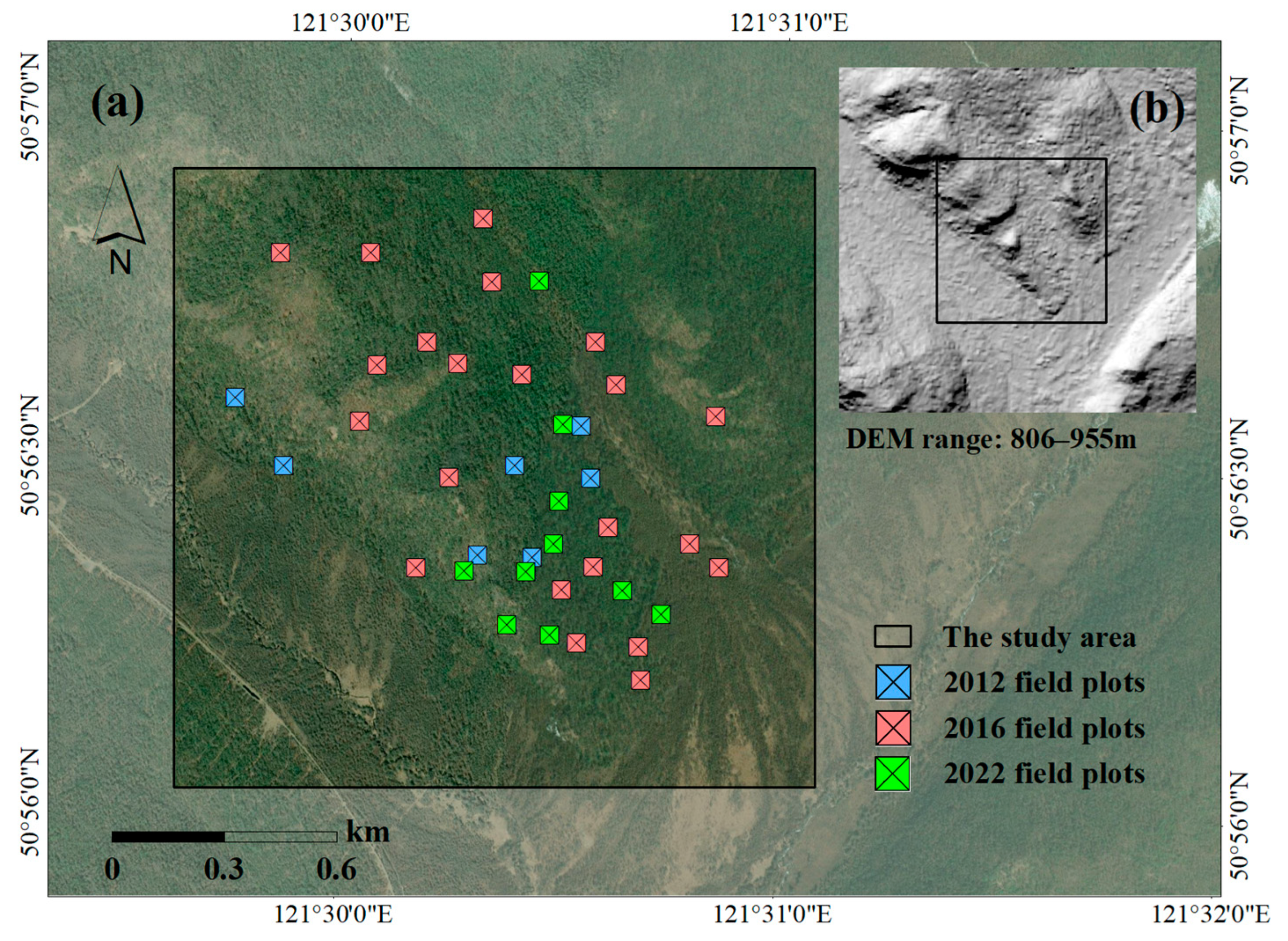
2.1. Study Area

The study area is at the Genhe ecological reserve (50°56′~50°57′N, 121°30′~121°31′E), which is located in the western part of the Greater Khingan Mountains (GKM), Inner Mongolia Autonomous Region, China (Figure 1). The average annual temperature is −5.3 °C, and the annual rainfall is 424 mm. The study area has a typical cold temperate continental monsoon climate, with an area of approximately 282 ha. This region is a natural secondary forest with typical single-layer stands, dominated by larch (Larix gmelinii (Rupr.) Kuzen.) with a small amount of birch (Betula platyphylla Suk.).

2.2. Field Plot Data

A total of 39 plots of 30 m × 30 m were surveyed in the study area, with 7, 22, and 10 plots investigated in 2012, 2016, and 2022, respectively. The subcompartment data in 2012 provided auxiliary information such as forest age groups at the subcompartment scale in each survey. The plot surveys were conducted shortly before and after LiDAR data collection. In each plot, the diameter at breast height (DBH), tree height, and crown width of trees with DBHs greater than 5 cm were measured. The four corner coordinates of the plots were recorded using a differential GPS device. The position of each tree was recorded for 8 of the 10 plots surveyed in 2022. In this process, a total station was directly positioned on the tree trunk to obtain the relative coordinates of each tree, and at the same time, the four corner coordinates of the plot were located and matched with the DGPS positioning points.

The AGB value for each measured tree was estimated based on its DBH using the local ASM equation established for the western GKM in a previous study [41]. Eight plots with tree positions were used to verify the accuracy of the ITS algorithm described in Section 2.4 and to calibrate the LiDAR-based AGB model detailed in Section 2.5. This dataset is referred to as the Tree-level Plot Data (TPD) for brevity. Additionally, we aggregated the individual tree AGB within each of the 39 plots to produce the plot-level AGB, which was employed to assess the accuracy of the plot-level AGB estimates discussed in Section 2.7. This dataset is referred to as the Plot-level Plot Data (PPD) for brevity.

We estimated the AGB change for each tree according to the published species-specific DBH growth curves for larch and birch [42] in the western GKM region. The AGB of each tree in the TPD was extrapolated to 2016 and 2012, respectively. Similarly, the AGB in the PPD was extrapolated to two other years where the AGB was unknown. A summary of detailed TPD and PPD is listed in

Table 1. Summary statistics of field plot data.

	2012		2016		2022
	Range	Mean	Range	Mean	Range	Mean
Tree-level Plot Data (TPD)
DBH/cm	2.9–40.6	14.9	3.8–41.2	16.0	5.0–42.0	17.5
Tree-level AGB/kg	1.44–909.7	79.9	2.7–944.6	91.2	5.1–992.4	107.5
Plot-level Plot Data (PPD)
DBH/cm	8.6–16.2	11.1	9.4–16.9	11.8	10.6–18.0	13.0
Plot-level AGB/(Mg/ha)	32.6–176.9	91.9	38.1–188.7	103.0	50.6–209.0	119.9

Note: The value of TPD is at the tree level and the value of PPD is at the plot level.

.

2.3. Remote Sensing Data Acquisition and Processing

The LiDAR data in the study area were acquired during the leaf-on growing season, and a total of three data acquisitions were carried out. In August 2012, a Leica ALS60 sensor was used to acquire ALS data (ALS2012) at an altitude of approximately 2700 m with a pulse repetition frequency of 300 kHz. The ALS data from August 2016 (ALS2016) were collected using a Riegl LMS-Q680i scanner mounted on the LiCHy airborne system of the Chinese Academy of Forestry at an altitude of approximately 2200 m with a 200 kHz pulse repetition frequency. In August 2022, a LiAir 1350 sensor was mounted on the DJI M600 PRO unmanned aerial vehicle (UAV) to obtain the ULS data (ULS2022) at an average altitude of 200 m with a 350 kHz pulse repetition frequency. At the same time, this UAV equipped with an RGB camera collected true-color images with a resolution of 0.1 m across the entire study area. The final LiDAR data were delivered by the vendor in LAS format, and the average pulse densities in 2012, 2016, and 2022 were 5.2 pulses/m², 2.6 pulses/m², and 146.2 pulses/m², respectively. The pulse density represents the density of first returns, which are more sensitive to the forest canopy. The ULS2022 data were covered by both ALS2012 and ALS2016, and therefore, the overlapping areas were retained for further analysis (Figure 1a). The detailed scanner properties and flight parameters for the three acquisitions are listed in

Table 2. Characteristics of three LiDAR data acquisitions.

Parameters	ALS2012	ALS2016	ULS2022
Acquisition time	30 August 2012	28 August 2016	20 August 2022
Sensor type	Leica ALS60	Riegl LMS-Q680i	LiAir 1350
Laser pulse frequency (kHz)	300	200	350
Flying altitude (m)	2700	2200	200
Scanning angle (°)	±35	±30	±45
Average pulse density(pulses/m2)	5.2	2.6	146.2
Wavelength (nm)	1064	1550	1550

.

We preprocessed the raw LiDAR data into normalized point clouds and CHMs. To avoid the bias of canopy height caused by topographic changes and enhance comparability among the datasets, the point cloud data for the three acquisitions were normalized using the 2022 digital terrain model (DTM) because the ULS2022 has the highest pulse density. The ULS2022 data were classified as ground and non-ground using a cloth simulation filter algorithm [43], and a DTM was fitted based on the ground returns, producing a raster of 0.3 m resolution. Next, the ALS2012 and ALS2016 data were normalized by subtracting the height of the DTM in 2022.

We used the method of Cao et al. [18] to co-register the three datasets based on a road through the study area to eliminate the systematic shifts in the heights among the three LiDAR acquisitions. The ULS2022 data were used as the benchmark. The mean height difference between 2012 and 2022 was 3.5 cm, and between 2016 and 2022 was 3 cm. As a result, the 2012ALS and 2016ALS were shifted by mean differences, respectively. To obtain a smoother CHM raster, the normalized point clouds were rasterized into CHMs using the point-to-raster (p2r) interpolation algorithm [44]. The ULS2022 data was interpolated to CHM at 0.3 m resolution, while ALS2012 and ALS2016 were interpolated at 1 m resolution, considering the limitation of pulse densities. All processing of the LiDAR point cloud data was performed using the lidR package [45].

2.4. Individual Tree Segmentation

Using UAV RGB images, 2022 CHM, and tree location coordinates, we manually delineated all visible crowns in the TPD and matched the measured DBH, tree height, and tree crown width for each tree. To ensure consistency in ITS for multitemporal LiDAR data, the ITS routine was used to identify individual trees from the ULS2022 data only. Subsequently, the polygons of the automatically delineated tree crowns were overlayed onto the ALS2012 and ALS2016.

In order to find the most suitable ITS techniques by weighing the time efficiency and accuracy of the algorithm, we tested two types of ITS techniques: a point cloud-based approach developed by Li et al. [46] (li2012) and a raster-based approach developed by Dalponte et al. [28] (dalponte2016). The li2012 algorithm employs a top-to-bottom approach to segment the normalized point cloud directly. This is a commonly used individual tree-segmentation technology based on point clouds that has been successfully demonstrated to be applied in various forest types [47,48,49]. The dalponte2016 algorithm relies on seed points to identify treetops by individual tree detection (ITD) and determines the canopy boundaries through a region-growing algorithm. Therefore, ITD is crucial to the accuracy of the dalponte2016 algorithm. We considered three local maximum filters to implement ITD. The first method was applied with a fixed size window of 1.5 m, 2 m, and 2.5 m (dalponte2016-FW). The second method used one variable window (dalponte2016-VW), where the window size was adjusted based on field-measured crown width and tree height using a regression equation. However, to mitigate omission errors, we used the 95% prediction interval of the regression equation instead of the original equation when determining the variable window size [50]. Additionally, a minimum threshold of 0.5 m was set to limit outliers (Figure 2a). The third method was two variable windows developed by canopy structural heterogeneity. In the presence of different levels of canopy structure heterogeneity, trees exhibit varying responses to resource competition, leading to differences in crown shape and size across heterogeneous stands. Recently, Valbuena et al. [51] calculated the Gini coefficient (GC) by LiDAR height. They proved that GC is a key indicator to characterize the canopy structure properties of the boreal forest ecosystem and can characterize the degree of variation in tree height and canopy density at different locations from a three-dimensional perspective. Adnan et al. [52] determined that a threshold of GC = 0.33 has the ability to stratify homogeneous and heterogeneous forest stands through mathematical proof, and we tested whether this threshold improves the accuracy of ITD. We calculated the GC of 2022 CHM for each TPD plot according to an unbiased estimator developed by Glasser [53] (Equation (1)) and divided TPD plots into two groups (GC < 0.33, n = 4; GC ≥ 0.33, n = 4) according to the threshold of 0.33 to represent low or high levels of canopy heterogeneity. The field-measured crown width and tree height from the two groups of TPD plots were used to fit the variable window equation, respectively (dalponte2016-GCVW), according to the second method (Figure 2b). The treetops identified through the aforementioned three methods were used as seed points in dalponte2016.

$$\mathrm{Gini}\mathrm{coefficient}=\frac{n}{n-1}\frac{{{\displaystyle \sum }}_{i=1}^n{{\displaystyle \sum }}_{\mathrm{j}=1}^{\mathrm{n}}\left|h_i-h_j\right|}{{2n}^2\overline{h}}$$

(1)

where $h_i$ is the value of $i\text{-}\mathit{th}$ 2022 CHM pixels inside the plot; $h_j$ is the value of $j\text{-}\mathit{th}$ 2022 CHM pixels inside the plot; $\overline{h}$ is the mean value of 2022 CHM pixels inside the plot; $n$ is the number of 2022 CHM pixels inside the plot.

We assessed the performance of ITS by comparing the IoU value (Equation (2)) between the manually delineated crowns (${\mathrm{M}}_{\mathrm{DC}}$) and the automatically delineated crowns (${\mathrm{A}}_{\mathrm{DC}}$) [54]. The IoU ≥ 0.5 was viewed as true positive (TP). ${\mathrm{A}}_{\mathrm{DC}}$ that failed to match with ${\mathrm{M}}_{\mathrm{DC}}$ were classified as false positives (FP), while ${\mathrm{M}}_{\mathrm{DC}}$ without corresponding ${\mathrm{A}}_{\mathrm{DC}}$ was viewed as false negatives (FN). Finally, TP, FP, and FN were used for calculating recall (Equation (3)), precision (Equation (4)), and F-score (Equation (5)). We compared the accuracy of several ITS methods and determined the best method for the subsequent steps.

$$\mathrm{IoU}\left({\mathrm{M}}_{\mathrm{DC}}{,\mathrm{A}}_{\mathrm{DC}}\right)=\frac{{\mathrm{M}}_{\mathrm{DC}}\cap {\mathrm{A}}_{\mathrm{DC}}}{{\mathrm{M}}_{\mathrm{DC}}\cup {\mathrm{A}}_{\mathrm{DC}}}$$

(2)

$$\mathrm{Recall}=\frac{\mathrm{TP}}{\mathrm{TP}+\mathrm{FN}}$$

(3)

$$\mathrm{Precision}=\frac{\mathrm{TP}}{\mathrm{TP}+\mathrm{FP}}$$

(4)

$$\mathrm{F}\text{-}\mathrm{score}=2\times \frac{\mathrm{Precision}\times \mathrm{Recall}}{\mathrm{Precision}+\mathrm{Recall}}$$

(5)

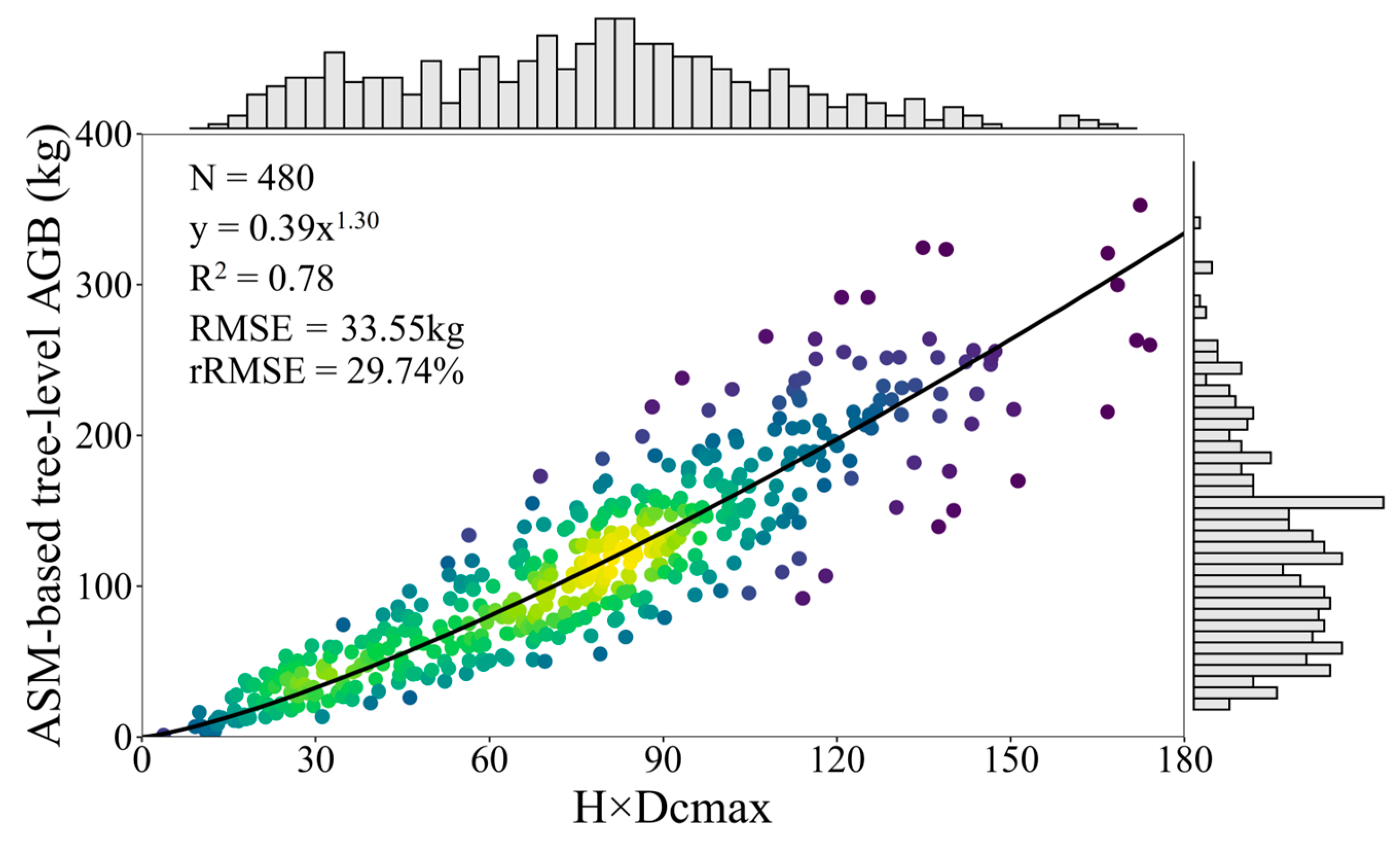
2.5. LiDAR-Based Tree AGB Model

LiDAR-based AGB models rely on metrics that both ULS and ALS can extract. Jucker et al. [8] quantified the AGB of individual trees using tree height and crown width, which could be derived by LiDAR. The model followed a power-law function, which was fitted by log-transformed, binned data:

$${\mathrm{AGB}=\alpha \times (\mathrm{H}\times \mathrm{CW})}^{\beta }$$

(6)

where $\mathrm{H}$ is the tree height; $\mathrm{CW}$ is the crown width; $\alpha$ and $\beta$ are different among plant clades and fitting to the local data is the most accurate. We fitted the model using correctly matched trees to estimate tree-level AGB. The H was determined by extracting the maximum height within the crown polygon. The CW was a crucial parameter in the model. However, since the crown polygons of each tree in ALS2012 and ALS2016 were determined by ULS2022, the differences in sensor, flight patterns, and pulse density led to greater uncertainty in CW estimation. The small changes in CW might not have been adequately captured. Therefore, we proposed a metric Dcmax to replace CW in Equation (7) through the following steps:

-

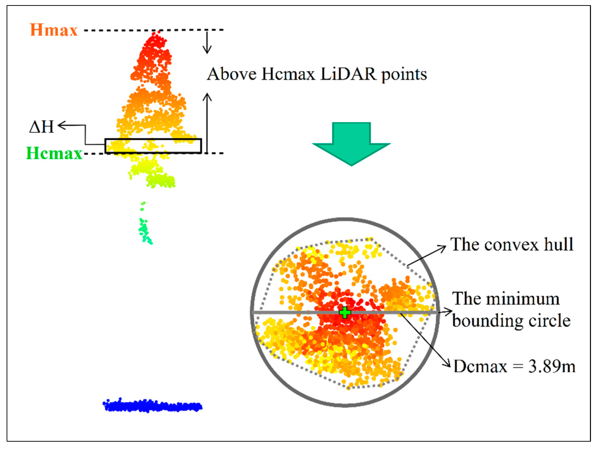
First, the ULS2022 point cloud above 2 m of each tree was segmented into horizontal slices using a height interval ($\Delta \mathrm{H}$), which was set to 1 m heuristically.

-

For each slice, the points were projected onto a horizontal plane, and the alpha-shape method was used to obtain its convex hull. The area of the convex hull was then calculated.

-

The slice with the maximum area of the convex hull was identified, and its height above the ground (Hcmax) was determined. All the points above Hcmax were projected onto the horizontal plane. Similarly, a convex hull was generated for the projected points, and the diameter of the minimum bounding circle of this convex hull was viewed as Dcmax in 2022 (Figure 3).

-

The Hcmax was applied to each tree of ALS2012 and ALS2016, and the Dcmax in 2012 and 2016 is extracted according to the third step.

$${\mathrm{AGB}=\alpha \times (\mathrm{H}\times \mathrm{Dcmax})}^{\beta }$$

(7)

The manually delineated TPD crowns matched with the automatically ITS-delineated 2022 crowns were used to fit the model (Equation (7)). The ASM-based AGB of each TPD tree was considered the dependent variable, and LiDAR-based H and Dcmax in 2022 were considered the independent variables. The AGB model was then fitted to the log-transformed, binned data. The prediction accuracy of the model was evaluated through ten-fold cross-validation using the coefficient of determination (R²; Equation (8)), root mean square error (RMSE; Equation (9)), and relative root mean square error (rRMSE; Equation (10)). The values of R², RMSE, and rRMSE were calculated as follows:

$$R^2=1-\frac{{{\displaystyle \sum }}_{i=1}^n{{(x}_i-\widehat{x_i})}^2}{{{\displaystyle \sum }}_{i=1}^n{{(x}_i-\overline{x_i})}^2}$$

(8)

$$\mathrm{RMSE}=\sqrt{\frac{1}{n}{\displaystyle \sum }_{i=1}^n{{(x}_i-\widehat{x_i})}^2}$$

(9)

$$\mathrm{rRMSE}=\frac{\mathrm{RMSE}}{\overline{x}}\times 100\%$$

(10)

where $n$ is the number of trees, $i$ is the tree number, $x_i$ is the ASM-based AGB value for tree $i$, $\widehat{x_i}$ is the predicted AGB value for tree $i$, and $\overline{x_i}$ is the mean ASM-based AGB value for all trees.

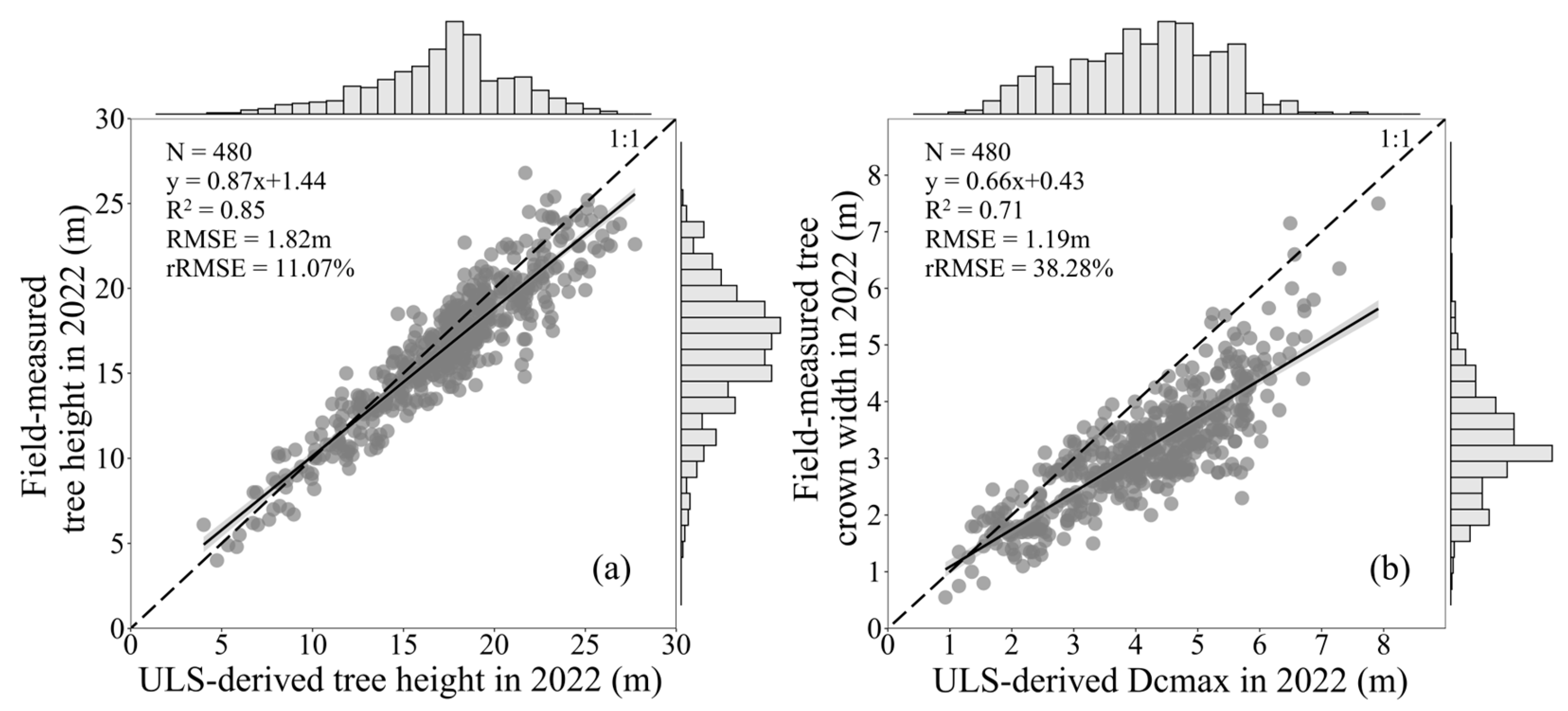
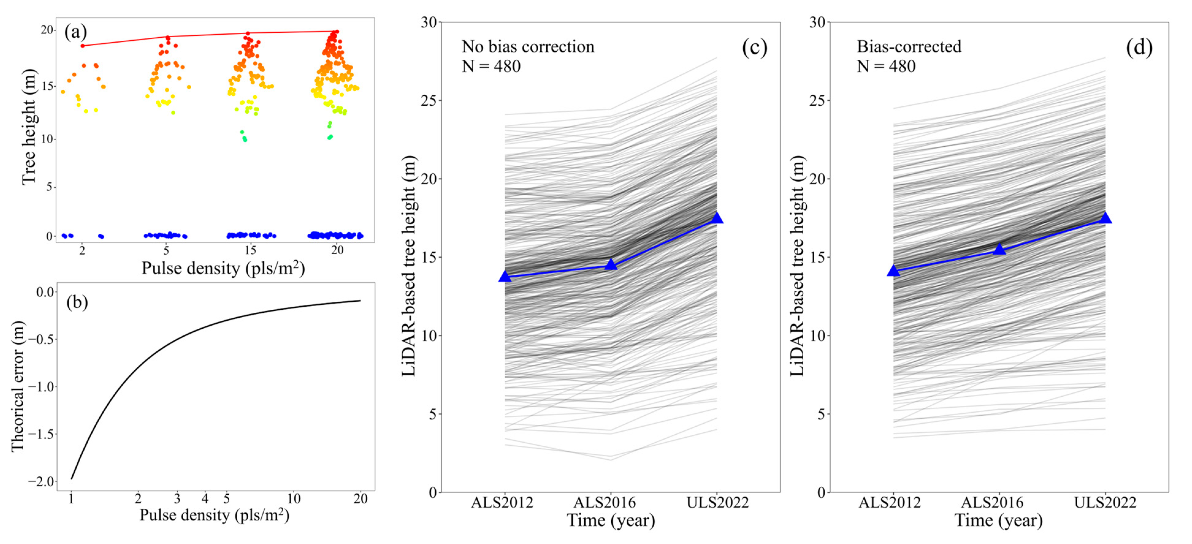
2.6. Correcting Biases for Tree Height and Dcmax

Roussel et al. [55] demonstrate that LiDAR-based metrics do not provide absolute values due to their dependency on various factors. These factors include not only the forest structure but also the characteristics of the LiDAR device, its settings, and the pattern of flight. The LiDAR-based tree heights and Dcmax have a tendency to be underestimated at a low pulse density because LiDAR tends to miss treetops [56], and such biases may not always be trivial. The lower the pulse density, the larger the underestimation bias [22]. Given the differing pulse densities among the three LiDAR data acquisitions, it becomes crucial to correct biases to accurately track individual tree growth. We considered the ULS2022 with the highest pulse density to provide unbiased estimates of H and Dcmax. We randomly selected 20 trees from ULS2022 within the TPD to quantify the relationship between biases and tree-level metrics.

We refer to the method of Roussel et al. [55] to correct the tree height extracted by ALS2012 and ALS2016. The method mathematically predicted the underestimated biases of tree heights using a probability model that simultaneously considered pulse density, sampling area, and canopy shape. A recursive function was used to describe the relationship between the probability of a pulse returning from a specified height and the expected value of the treetop height by gradually decreasing the pulse densities. The 20 trees were used to quantify the underestimation biases of tree height. More details of this method have been provided by Roussel et al. [55].

Since Dcmax cannot be modeled according to the probability of returning height, an empirical model was used to correct for biases. The 20 trees were thinned to a series of lower pulse densities with a step size of 0.2 pulses/m², and this process was repeated 10 times to take the average value to eliminate randomness in the point cloud thinning. The mean values of each 0.2 pulses/m² interval for 20 trees were treated as bin data, and a logarithmic model was used to build the quantitative relationship between pulse densities and underestimation biases.

2.7. Spatial Extrapolation and AGB Dynamic Analysis

After correcting the biases for tree height and Dcmax estimated by ALS2012 and ALS2016, the wall-to-wall tree-level AGB for three acquisitions (${\mathrm{AGB}}_{12}$, ${\mathrm{AGB}}_{16}$, and ${\mathrm{AGB}}_{22}$) and the AGB change for every two acquisitions (${\mathrm{AGB}}_{22–16}$, $\Delta {\mathrm{AGB}}_{16–12}$, and $\Delta {\mathrm{AGB}}_{22–12}$) were calculated across the study area. The accuracy of forest AGB estimation was then assessed at two levels. At the tree level, correctly matched trees in TPD were used to evaluate the accuracy between field- and LiDAR-based AGB. At the plot level, tree-level AGB was aggregated spatially within the PPD range, which was used to evaluate the accuracy between field- and LiDAR-based AGB. Subsequently, a series of 30 × 30 m grids corresponding to the dimensions of the field plots were generated across the entire study area, and tree-level AGB was aggregated into the grids to estimate the wall-to-wall plot-level AGB and its dynamics maps.

In order to explore environmental factors affecting AGB growth rates at the plot level across the landscape, we investigated the relationship between AGB changes and forest age groups, topography, canopy density, and canopy structural heterogeneity. We calculated the relative change rate of the AGB for every two acquisitions ($\Delta {\mathrm{AGB}\%}_{22–16}$, $\Delta {\mathrm{AGB}\%}_{16–12}$, and $\Delta {\mathrm{AGB}\%}_{22–12}$) as follows:

$$\Delta {\mathrm{AGB}\%}_{{\mathrm{t}}_2-{\mathrm{t}}_1}=\frac{{(\mathit{AGB}}_{t_2}-{\mathit{AGB}}_{t_1}{)/\mathit{AGB}}_{t_1}}{t_2-t_1}\times 100\%$$

(11)

where ${\mathit{AGB}}_{t_1}$ and ${\mathit{AGB}}_{t_2}$ are the forest AGB estimates for the years $t_1$ and $t_2$, respectively.

In terms of the topographic data, we resampled the DTM to 30 m to correspond to the plot size. The aspect was calculated using QGIS and divided into four categories: sunny slope (0~45 degrees and 315~360 degrees), semi-sunny slope (45~90 degrees and 270~315 degrees), semi-shady slope (90~135 degrees and 225~270 degrees), and shady slope (135~225 degrees). The elevation was divided into three categories according to the elevation range in the study area: low (806~850 m), median (850~900 m), and high (900~955 m). Information on forest age groups (young, middle-aged, near-mature, and mature) was obtained from the subcompartment data. The canopy density was determined by calculating the ratio of the number of first returns above 2 m to the total number of first returns. The canopy structure heterogeneity was characterized by the GC of the CHM (Equation (1) within each 30 m grid. In the analysis of $\Delta \mathrm{AGB}\%$, the initial stand status was taken into consideration, as canopy density and GC tend to change with forest growth. For instance, the canopy density and GC in 2016 were used to access the $\Delta {\mathrm{AGB}\%}_{22–16}$.

To determine how well environmental factors contributed to explaining $\Delta {\mathrm{AGB}\%}_{{\mathrm{t}}_2-{\mathrm{t}}_1}$ across the landscape, the Boruta algorithm [57] ranked the importance of all factors, where forest age groups, aspect, and elevation were considered categorical variables, and the canopy density and GC were considered continuous variables. The Boruta algorithm is built based on the random forest algorithm and evaluates the significance of the explanatory variables using Z scores.

3. Results

3.1. ITS Algorithms Accuracy Comparison

The results of the ITS are presented in

Table 3. Comparison of accuracy metrics for all ITS methods.

ITS Methods	Recall	Precision	F-Score	Time (s)
li2012	0.45	0.53	0.49	18.8
dalponte2016-FW
Window size: 1.5 m	0.58	0.55	0.56	4.8
Window size: 2 m	0.56	0.64	0.60	4.4
Window size: 2.5 m	0.47	0.72	0.57	3.9
dalponte2016-VW	0.66	0.68	0.67	5.5
dalponte2016-GCVW	0.80	0.73	0.76	5.8

and Figure 4. Among all the ITS methods, li2012 exhibited the lowest accuracy, and its operation time significantly exceeded that of other methods. In the case of dalponte2016-based methods, fixed window filtering required less operation time compared to variable window filtering. However, variable window filtering had a higher accuracy and F-score compared to fixed window filtering. It is worth noting that as the size of the fixed window increased, the recall gradually decreased but the precision increased.

Among all the methods, the dalponte2016-GCVW method emerged as the most effective, exhibiting the highest accuracy and F-score. Compared to dalponte2016-VW, dalponte2016-GCVW demonstrated a substantial improvement in recall ($\Delta \mathrm{recall}=0.14$) by incorporating canopy structural heterogeneity. Moreover, upon the visual inspection of both low- and high-canopy structural heterogeneity forest stands, it was observed that the omission error was significantly reduced in the high heterogeneity stand (Figure 4(f2)). Taking time efficiency and accuracy into consideration, we ultimately selected dalponte2016-GCVW for further analysis. A total of 480 trees were correctly matched during the process of pairing the automatically delineated crowns with the manually delineated crowns using IoU values. These trees were utilized to validate the LiDAR-based AGB model.

3.2. LiDAR-Based AGB Model Results and Accuracy Evaluation

Among the 480 correctly matched trees selected from TPD, the average tree height derived by ULS was 0.82 m higher than the measured tree height, which was usually attributed to the occlusion of treetops observed by surveyors from the ground. Furthermore, the magnitude of this error gradually increased as the height of the tree increased (Figure 5a). Dcmax shows a linear relationship with the field-measured crown width. However, since Dcmax was designed as a metric resembling the circumscribed circle of the crown width, it tended to be larger than the measured crown width (Figure 5b). In this study, the tree height and Dcmax derived from LiDAR showed a strong correlation with the field-measured data, demonstrating the feasibility of applying LiDAR-based tree metrics to the AGB model.

When Equation (7) is fitted to log-transformed binned data of 480 correctly matched trees, we obtained the following relationship between $\mathrm{H}\times \mathrm{Dcmax}$ and ASM-based tree-level AGB (Figure 6):

$$\mathrm{AGB}=0.39{\times (\mathrm{H}\times \mathrm{Dcmax})}^{1.30}$$

(12)

The 10-fold cross-validation results showed that the model achieved high accuracy in estimating AGB, with R² and rRMSE of 0.78 and 29.74%, respectively. It is worth noting that $\mathrm{H}\times \mathrm{Dcmax}$ consistently increased with rising AGB without any indication of saturation within the value range of the data. The LiDAR-based AGB model provided reliable estimates of tree-level AGB in our study area.

3.3. H and Dcmax Correction Results

Figure 7a and Figure 8a show the sensitivity of tree height and Dcmax to pulse densities. As the pulse density decreases, the tree-level metrics estimates gradually decrease, indicating a larger underestimation bias at lower pulse densities. Before correction, the average value of $\Delta {\mathrm{H}}_{16–12}$ was 0.78 m (average annual 0.20 m), $\Delta {\mathrm{H}}_{22–16}$ was 2.14 m (average annual 0.37 m); the average value of $\Delta {\mathrm{Dcmax}}_{16–12}$ was 0.09 m (average annual 0.02 m), and $\Delta {\mathrm{Dcmax}}_{22–16}$ was 0.34 m (average annual 0.06 m). The deviation in pulse density led to inconsistent growth rates of tree height and Dcmax between the two periods estimated by LiDAR, and these errors were further amplified when extrapolated to estimate AGB. Given that ALS2016 had the lowest average pulse density, we even found that some tree heights and Dcmax estimated by ALS2016 were lower than those of ALS2012, which contradicted the expected trend (Figure 7c and Figure 8c). The 20 reference trees were utilized to fit both probability and empirical models (Figure 7b and Figure 8b). The probability model offered a mechanistic explanation of the underlying sampling process [55]. Although the empirical model was locally efficient, Dcmax was accurately modeled using binned data at various pulse densities, with an R² value of 0.96 ($y=0.11\times \ln \left(x\right)-0.35$). As expected, after correcting biases of tree height and Dcmax using probabilistic and empirical models, these two metrics showed more consistent growth patterns (Figure 7d and Figure 8d) ($\Delta {\mathrm{H}}_{16–12}$ = 1.02 m, $\Delta {\mathrm{H}}_{22–16}$ = 1.65 m, average annuals were 0.26 m and 0.28, respectively; $\Delta {\mathrm{Dcmax}}_{16–12}$ = 0.14 m, $\Delta {\mathrm{Dcmax}}_{22–16}$ = 0.20, average annuals were 0.04 m and 0.03 m, respectively). The LiDAR effectively captured the growth trajectory of each tree, demonstrating the effectiveness of multitemporal LiDAR data in monitoring tree growth at a fine scale.

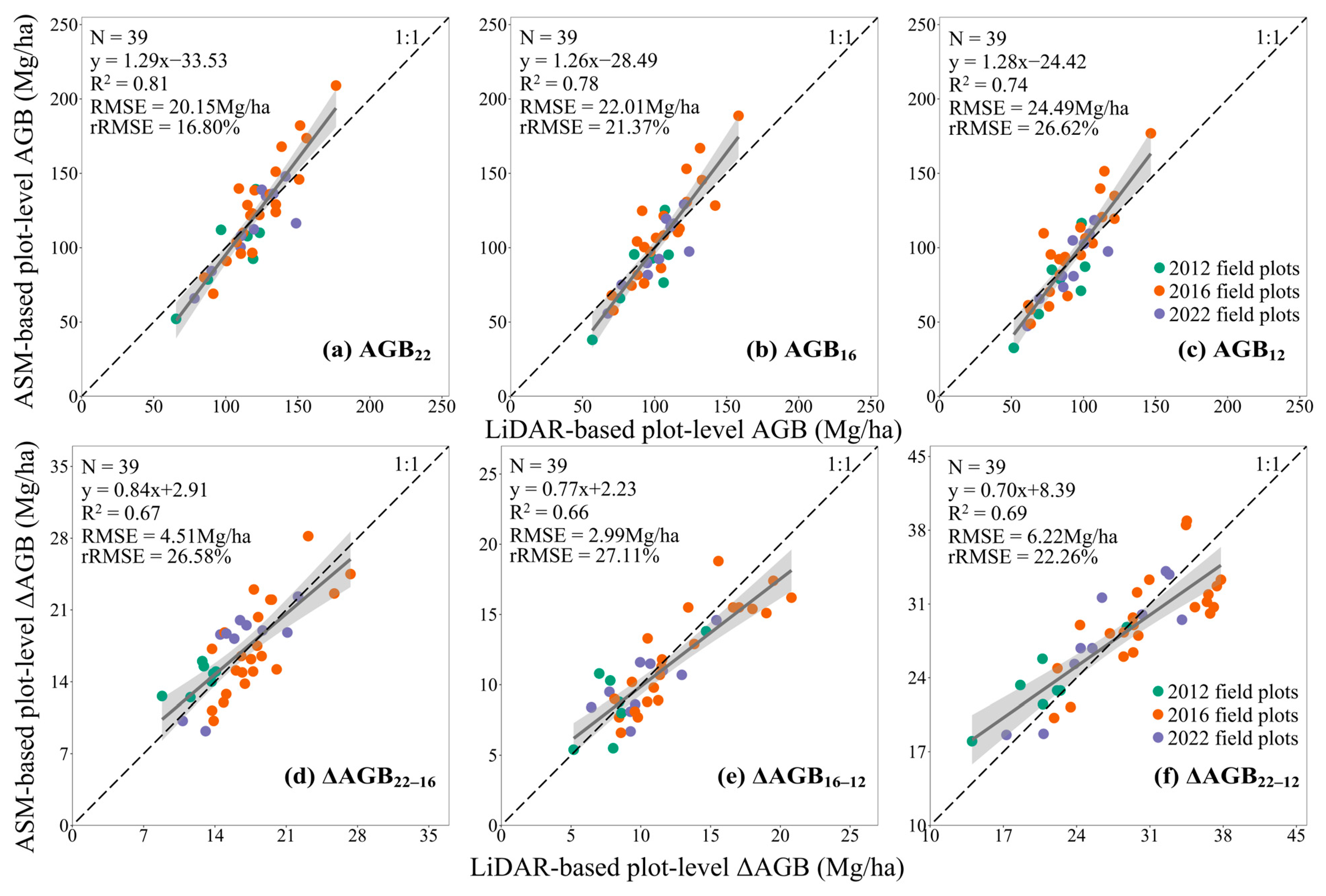
3.4. Assessment of AGB Changes at the Tree- and Plot-Level

The comparisons between the ASM-estimated and model-predicted AGB and its changes for 480 correctly matched trees are shown in Figure 9. The LiDAR estimations demonstrated reasonable accuracy in predicting tree-level AGB from 2012 to 2022 (Figure 9a–c), explaining 72% to 80% of the variance of ASM-based AGB. However, as the AGB increased, the estimation error of the AGB became more pronounced. When calculating AGB changes for every two acquisitions, the LiDAR-based $\Delta \mathrm{AGB}$ explained 62% to 70% of the variance of the ASM-based $\Delta \mathrm{AGB}$. The estimations of $\Delta {\mathrm{AGB}}_{22–12}$ had a higher correlation than the $\Delta {\mathrm{AGB}}_{22–16}$ and $\Delta {\mathrm{AGB}}_{16–12}$.

When the LiDAR-based tree-level AGB was aggregated spatially within the PPD, the estimations accounted for 74% to 81% of the variance of the ASM-based AGB. Notably, the AGB estimation results at the plot level exhibited higher accuracy compared to the individual tree level. LiDAR-based AGB demonstrated a tendency to overestimate at lower values and underestimate at higher values (Figure 10a–c). However, when estimating $\Delta \mathrm{AGB}$, they showed the opposite pattern, underestimating at lower values and overestimating at higher values (Figure 10d–f).

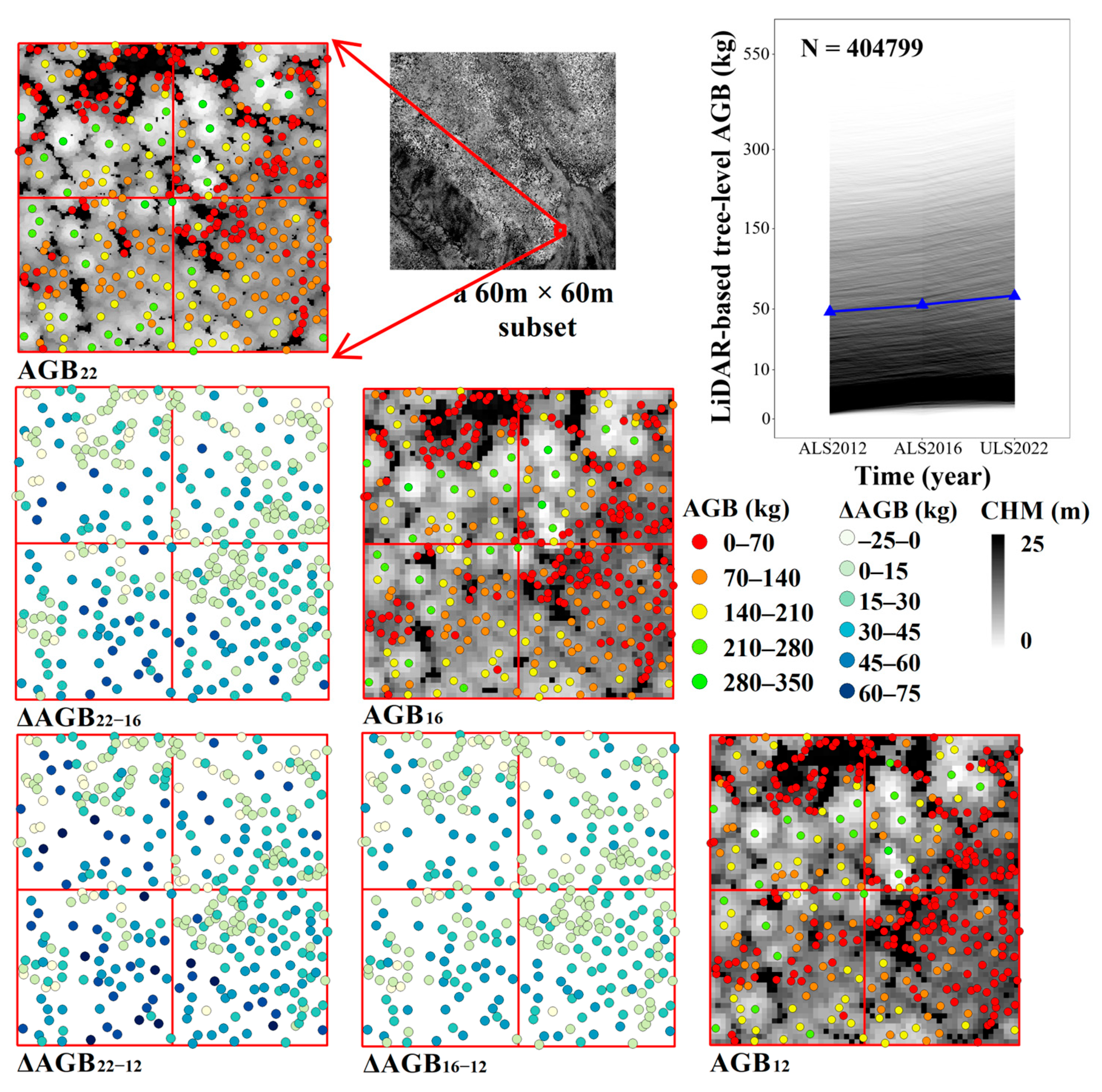
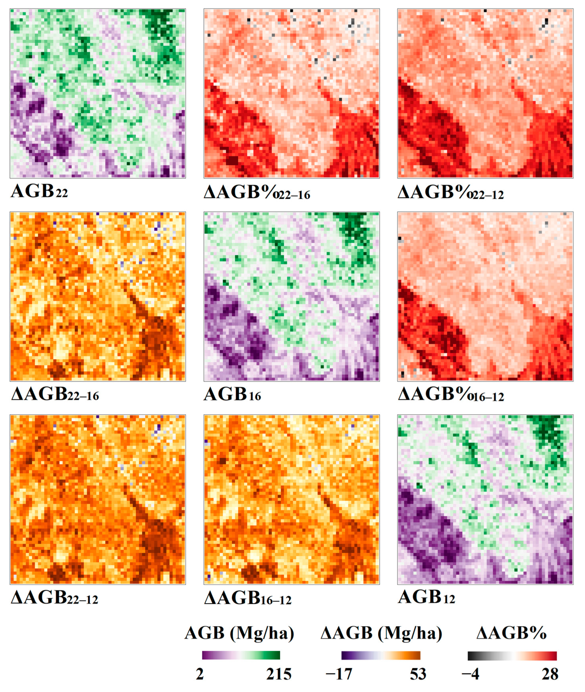
3.5. Spatiotemporal Variation in AGB

A total of 404,799 trees were segmented using the dalponte2016-GCVW method. After the pulse density correction for tree height and Dcmax, 92% of the trees (372,278 trees) exhibited normal growth. Wall-to-wall maps of tree-level AGB and its dynamics across the entire study area were predicted (Figure 11). The average values of AGB, tree height, and Dcmax in 2012, 2016, and 2022 for all trees were 40.24 kg/11.21 m/3.25 m, 49.38 kg/12.19 m/3.36 m, and 62.54 kg/13.73 m/3.56 m, respectively. The average annual changes in AGB, tree height, and Dcmax were 2.23 kg, 0.25 m, and 0.03 m, respectively. When aggregating the tree-level AGB into a 30 m grid, the wall-to-wall maps of plot-level AGB and its dynamics across the entire study area are shown in Figure 12. Overall, the annual average of plot-level $\Delta \mathrm{AGB}$ was estimated at 2.6 Mg/ha.

The importance rankings of environmental factors on the plot-level $\Delta \mathrm{AGB}\%$ for every two acquisitions determined by the Boruta algorithm are shown in

Table 4. The importance ranking of environmental factors on the plot-level $\Delta \mathrm{AGB}\%$ for each two time periods.

Environmental Factors	$\Delta {\mathbf{AGB}\%}_{22–16}$	$\Delta {\mathbf{AGB}\%}_{16–12}$	$\Delta {\mathbf{AGB}\%}_{22–12}$
Forest stand age	10%	12%	9%
Aspect	3%	2%	4%
Elevation	8%	5%	3%
Canopy density 2012		9%	8%
Canopy density 2016	5%
GC 2012		32%	30%
GC 2016	34%

. GC had a significant impact on the AGB growth rates, and the significance was much larger than the remaining four factors. The forest stand age was usually the second strongest predictor of the $\Delta \mathrm{AGB}\%$. The responses of aspect and elevation to the $\Delta \mathrm{AGB}\%$ were relatively weaker.

4. Discussion

LiDAR has been extensively demonstrated to enable accurate spatial predictions of tree-level AGB, while multitemporal LiDAR has emerged as a powerful tool for monitoring dynamic changes in forest resources at the grid level. Much of the prior research has primarily focused on these areas [18,58,59,60]. In this study, we improved the accuracy of individual tree segmentation algorithms by taking advantage of canopy structural heterogeneity and achieved stable estimation of AGB by eliminating the biases of inconsistent multitemporal LiDAR pulse densities on tree metrics. Furthermore, we evaluated the effectiveness of the multitemporal LiDAR for monitoring AGB at both the tree and plot levels, which require urgent attention. Accurate estimation of tree-level AGB dynamics plays an important role in explaining small-scale ecological processes and holds significant potential for enhancing forest management practices and formulating reasonable development plans.

4.1. Effectiveness and Applicability of ITS

The accuracy of ITS plays a crucial role in minimizing the uncertainty associated with tree-level AGB estimation. In our study, we address the challenges of under- and over-segmentation by capitalizing on canopy structural heterogeneity, particularly in complex forest stands. It is important to note that over-segmentation alone does not substantially impact AGB estimates. For instance, if we vertically bisect a tree and solely model AGB as a function of tree height, this can result in a significant overestimation of AGB. However, when we integrate crown width into the model, the resulting two trees from the bisection have half the crown width of the original tree, thereby alleviating the AGB estimation error caused by over-segmentation. Furthermore, our study area primarily comprises single-layer forest stands. This reduces the risk of underestimating stand-level AGB since multi-layered stands and undivided understory trees are not prevalent. Coomes et al. [27] identified that the under-segmentation of understory trees could lead to underestimations of stand-level AGB in multilayered tropical stands. Nevertheless, they have successfully employed a common correction factor to account for omission bias in AGB estimates, demonstrating an effective method to compensate for ITS limitations in certain ecosystems.

Numerous studies have developed a variety of techniques for ITS using ALS and ULS. However, despite the increasing number of methods, most of them have been developed using specific forest-structured datasets, thereby limiting their practical applicability. Yang et al. [49] compared the impact of various forest types on the accuracy of the ITS methods. Their findings revealed that contrary to the emphasis on forest density in some literature, it was forest homogeneity or heterogeneity that had a significant correlation with ITS accuracy. The forest stand heterogeneity is especially notable in mixed forests, where there are significant variations in canopy structure between conifers and broadleaves [39]. This heterogeneity brings more ITS errors of omission and commission [61,62]. Adnan et al. [52] have demonstrated that GC calculated by the LiDAR height based on deductive mathematical rules describing distributions could be used as auxiliary variables in the forest AGB model, and the threshold of GC = 0.33 had the ability to stratify homogeneous and heterogeneous stands. When stratifying the TPD by GC, we observed contrasting relationships between tree height and crown width in low and high heterogeneity (Figure 2b). Especially in highly heterogeneous stands, taller trees exhibited larger crown sizes, while smaller trees had smaller crown sizes. Variable window filtering based on GC could effectively quantify this variation, exhibiting higher accuracy compared to other methods (Table 3). This idea could even be applied to other ITS methods based on the distance threshold to enhance the adaptability of the ITS methods to different forest types. Furthermore, when ranking the importance of environmental factors at the plot level, it was found that GC significantly influenced the relative change rate of the AGB. It is important to emphasize that the availability of light and its interception by the dominant canopy are the primary factors that limit forest growth in boreal forests [51]. As individual trees grow, the canopies begin to touch and shade each other. During this phase, they exhibit varying responses to resource competition, resulting in inequalities in height and crown size. In addition, the diversity of canopy structure affects factors such as light intensity and soil moisture, which in turn have an impact on forest growth [40].

4.2. Inconsistencies among Multitemporal LiDAR Data

Monitoring forest growth utilizing multitemporal LiDAR data encounters numerous challenges and uncertainties, necessitating special attention to suppress the interference of external factors in order to reveal the true dynamic changes accurately [22,63]. Firstly, having a standardized ground reference is a prerequisite. It is crucial to correct the height bias between different LiDAR datasets, ensuring that heights are consistent over time and enabling meaningful comparisons. Different estimates of DTMs could arise from variations in LiDAR sensors, parameter settings, and flight modes. Yu et al. [64] demonstrated that the utilization of different DTMs in multitemporal LiDAR studies could introduce biases that were larger than the actual tree height growth in some cases. Therefore, we used the DTM obtained by ULS to normalize the point cloud data and eliminated the height deviation for three acquisitions.

Another important aspect to consider is addressing the sensitivity of pulse density to LiDAR metrics. Some research based on ABA has demonstrated that pulse density has no significant impact on forest attribute estimation at the plot level. This can be attributed to the sampling of laser scans according to a probability distribution, where LiDAR metrics exhibit similar vertical distribution patterns when aggregated at larger scales [19]. Tree-level metrics, such as tree height and crown width, are direct measurements obtained from LiDAR data and not statistical estimates. The point cloud data in 2016 had the lowest average pulse density, and we observed the inconsistent growth of tree-level metrics in the two time periods (Figure 7d and Figure 8d). This phenomenon deserves special attention, especially in coniferous forests. Our findings indicated that tree height and Dcmax could be reliably estimated when the pulse density was at least 10 pulses/m², while the estimation error increased rapidly when the pulse density fell below 5 pulses/m². This asymptotic relationship was similar to that found by Hirata [65]. We emphasize the need to address the density dependence of tree metrics, as failure to do so may limit the practical application of the ITA approach, particularly when using multitemporal LiDAR data collected with different sampling parameters for forest growth monitoring.

4.3. Availability of LiDAR-Based Tree AGB Model

The choice of an appropriate model form and tree metrics is crucial for the accurate evaluation of AGB and its dynamics. Jucker et al. [8] used destructively harvested trees and revealed strong correlations between AGB and both tree height and crown size. Ploton et al. [66] also demonstrated the effectiveness of incorporating crown size into the ASM for AGB estimation. The inclusion of canopy information in ASM is particularly valuable as a large portion of AGB is contributed by branches, enabling ASM to distinguish between trees of similar height but with varying crown sizes. Using the model with crown information has great promise for estimating tree-level AGB through remote sensing technologies, as conventional ASM frequently encounters saturation effects in AGB estimation. Du et al. [30] found a saturation trend between tree height and biomass index based on a sample of 124 larch trees from three different forest farms in Northeast China. However, when utilizing a LiDAR biomass index that contains crown information to predict AGB within the 0 to 400 kg range, no saturation was observed. This consistency with our research results further supports the validity of incorporating crown information in AGB estimation (Figure 6).

Zhao et al. [22] performed ITS on the LiDAR data for the four periods and matched the LiDAR trees from different acquisitions to calculate the tree height change within ten years. During the process of matching LiDAR trees, the variation in ITS results for different LiDAR acquisitions and the matching errors could complicate the analysis of multitemporal LiDAR data. In our study, we only applied the ITS routine to ULS2022 and overlayed the crown polygons on the other two LiDAR acquisitions. This processing framework helps mitigate omission errors in the matching process for analyzing multitemporal data. However, it comes at the cost of increased uncertainty in crown width estimates because the same crown extent will not capture the changes in crown width over time. Fortunately, we replaced the crown width with Dcmax and observed a strong correlation between the two metrics. Considering that the traditional crown width is calculated by projecting on the horizontal plane, we found the height of the point cloud slice with the maximum area to elevate the estimation of Dcmax into three-dimensional space (Figure 3). The ability of Dcmax to capture subtle changes in the canopy after pulse density correction demonstrates its stability as tree-level metrics.

The model form of Equation (7) provides a simple solution to quantify AGB at local regions since the model is easy to parameterize and verify. Brede et al. [35] used locally measured trees and ULS-derived metrics to parameterize this model and estimated tree-level AGB with rRMSE ranging from 51.94% to 116.89%. In our study, the accuracy of tree-level AGB estimation was better than their results (rRMSE: 24.48%~28.52%). It is worth noting that their research was conducted in temperate and tropical plots with complex and diverse tree species. Our study specifically targeted a boreal forest dominated by larch with a small amount of birch. Dalponte et al. [29] reported that there were no significant differences in tree-level AGB predicted by species-specific and non-species-specific models in forests with fewer tree species, such as boreal forests. Tree species information had a limited impact on the results. The next crucial step is to assess the performance of this AGB model across different tree species and various forest types.

5. Conclusions

In this study, we used multitemporal LiDAR data to estimate and map spatiotemporal variations of tree-level AGB over 10 years in the boreal natural secondary forests in the GKM region. We improved the accuracy of the individual tree segmentation algorithm by taking advantage of canopy structural heterogeneity. In addition, the probabilistic and empirical models corrected the biases of tree height and Dcmax caused by inconsistent multitemporal LiDAR pulse densities, and the tree-level AGB was aggregated spatially to the plot level to evaluate the estimation accuracy of AGB and its dynamics at different scales. The results showed that GC quantified the difference between tree height and crown width in heterogeneous stands, and was the most important environmental factor to explain the relative change rate of the AGB at the plot level across the entire study area. The LiDAR-based AGB model achieves high accuracy without saturation tendency (R² = 0.78, rRMSE = 29.74%). Individual tree-based approach estimates showed that the average annual changes in AGB, tree height, and Dcmax were 2.23 kg, 0.25 m, and 0.03 m, respectively. Overall, this study demonstrates the applicability of using multitemporal LiDAR data for mapping spatiotemporal variations of fine-scale forest dynamics, which are particularly valuable for carbon trading, REDD+, and other goals aimed at achieving climate mitigation through forest management across different levels. As individual tree segmentation algorithms, LiDAR data collection, and analysis platforms continue to advance and mature, ITA-based methods are expected to become one of the increasingly valuable solutions for monitoring forest dynamics.

References

1. Bonan, G.B. Forests and Climate Change: Forcings, Feedbacks, and the Climate Benefits of Forests. Science 2008, 320, 1444–1449. [Google Scholar] [CrossRef]
2. Pan, Y.; Birdsey, R.A.; Fang, J.; Houghton, R.; Kauppi, P.E.; Kurz, W.A.; Phillips, O.L.; Shvidenko, A.; Lewis, S.L.; Canadell, J.G.; et al. A Large and Persistent Carbon Sink in the World’s Forests. Science 2011, 333, 988–993. [Google Scholar] [CrossRef] [PubMed]
3. Lu, D.; Chen, Q.; Wang, G.; Liu, L.; Li, G.; Moran, E. A survey of remote sensing-based aboveground biomass estimation methods in forest ecosystems. Int. J. Digit. Earth 2016, 9, 63–105. [Google Scholar] [CrossRef]
4. Le Toan, T.; Quegan, S.; Davidson, M.W.J.; Balzter, H.; Paillou, P.; Papathanassiou, K.; Plummer, S.; Rocca, F.; Saatchi, S.; Shugart, H. The BIOMASS mission: Mapping global forest biomass to better understand the terrestrial carbon cycle. Remote Sens. Environ. 2011, 115, 2850–2860. [Google Scholar] [CrossRef]
5. Allouis, T.; Durrieua, S.; Véga, C.; Couteron, P. Exploiting fullwaveform lidar signals to estimate timber volume and above-ground biomass of individual trees. In Proceedings of the 2011 IEEE International Geoscience and Remote Sensing Symposium, Vancouver, BC, Canada, 24–29 July 2011; pp. 1251–1254. [Google Scholar]
6. Johnson, L.K.; Mahoney, M.J.; Bevilacqua, E.; Stehman, S.V.; Domke, G.M.; Beier, C.M. Fine-resolution landscape-scale biomass mapping using a spatiotemporal patchwork of LiDAR coverages. Int. J. Appl. Earth Obs. Geoinf. 2022, 114, 103059. [Google Scholar] [CrossRef]
7. Krofcheck, D.J.; Litvak, M.E.; Lippitt, C.D.; Neuenschwander, A. Woody biomass estimation in a southwestern US juniper savanna using lidar-derived clumped tree segmentation and existing allometries. Remote Sens. 2016, 8, 453. [Google Scholar] [CrossRef]
8. Jucker, T.; Caspersen, J.; Chave, J.; Antin, C.; Barbier, N.; Bongers, F.; Dalponte, M.; van Ewijk, K.Y.; Forrester, D.I.; Haeni, M. Allometric equations for integrating remote sensing imagery into forest monitoring programmes. Glob. Change Biol. 2017, 23, 177–190. [Google Scholar] [CrossRef]
9. Chave, J.; Réjou-Méchain, M.; Búrquez, A.; Chidumayo, E.; Colgan, M.S.; Delitti, W.B.C.; Duque, A.; Eid, T.; Fearnside, P.M.; Goodman, R.C. Improved allometric models to estimate the aboveground biomass of tropical trees. Glob. Change Biol. 2014, 20, 3177–3190. [Google Scholar] [CrossRef]
10. Demol, M.; Verbeeck, H.; Gielen, B.; Armston, J.; Burt, A.; Disney, M.; Duncanson, L.; Hackenberg, J.; Kükenbrink, D.; Lau, A. Estimating forest above-ground biomass with terrestrial laser scanning: Current status and future directions. Methods Ecol. Evol. 2022, 13, 1628–1639. [Google Scholar] [CrossRef]
11. Temesgen, H.; Affleck, D.; Poudel, K.; Gray, A.; Sessions, J. A review of the challenges and opportunities in estimating above ground forest biomass using tree-level models. Scand. J. For. Res. 2015, 30, 326–335. [Google Scholar] [CrossRef]
12. Badreldin, N.; Sanchez-Azofeifa, A. Estimating Forest Biomass Dynamics by Integrating Multi-Temporal Landsat Satellite Images with Ground and Airborne LiDAR Data in the Coal Valley Mine, Alberta, Canada. Remote Sens. 2015, 7, 2832–2849. [Google Scholar] [CrossRef]
13. Sun, G.; Ranson, K.J.; Guo, Z.; Zhang, Z.; Montesano, P.; Kimes, D. Forest biomass mapping from lidar and radar synergies. Remote Sens. Environ. 2011, 115, 2906–2916. [Google Scholar] [CrossRef]
14. Wulder, M.A.; Hermosilla, T.; White, J.C.; Coops, N.C. Biomass status and dynamics over Canada’s forests: Disentangling disturbed area from associated aboveground biomass consequences. Environ. Res. Lett. 2020, 15, 094093. [Google Scholar] [CrossRef]
15. Asner, G.P.; Mascaro, J.; Muller-Landau, H.C.; Vieilledent, G.; Vaudry, R.; Rasamoelina, M.; Hall, J.S.; van Breugel, M. A universal airborne LiDAR approach for tropical forest carbon mapping. Oecologia 2012, 168, 1147–1160. [Google Scholar] [CrossRef] [PubMed]
16. Næsset, E.; Gobakken, T.; Holmgren, J.; Hyyppä, H.; Hyyppä, J.; Maltamo, M.; Nilsson, M.; Olsson, H.; Persson, Å.; Söderman, U. Laser scanning of forest resources: The nordic experience. Scand. J. For. Res. 2004, 19, 482–499. [Google Scholar] [CrossRef]
17. Wulder, M.A.; Bater, C.W.; Coops, N.C.; Hilker, T.; White, J.C. The role of LiDAR in sustainable forest management. For. Chron. 2008, 84, 807–826. [Google Scholar] [CrossRef]
18. Cao, L.; Coops, N.C.; Innes, J.L.; Sheppard, S.R.J.; Fu, L.; Ruan, H.; She, G. Estimation of forest biomass dynamics in subtropical forests using multi-temporal airborne LiDAR data. Remote Sens. Environ. 2016, 178, 158–171. [Google Scholar] [CrossRef]
19. Hudak, A.T.; Strand, E.K.; Vierling, L.A.; Byrne, J.C.; Eitel, J.U.H.; Martinuzzi, S.; Falkowski, M.J. Quantifying aboveground forest carbon pools and fluxes from repeat LiDAR surveys. Remote Sens. Environ. 2012, 123, 25–40. [Google Scholar] [CrossRef]
20. Næsset, E.; Bollandsås, O.M.; Gobakken, T.; Gregoire, T.G.; Ståhl, G. Model-assisted estimation of change in forest biomass over an 11year period in a sample survey supported by airborne LiDAR: A case study with post-stratification to provide “activity data”. Remote Sens. Environ. 2013, 128, 299–314. [Google Scholar] [CrossRef]
21. Xu, D.; Wang, H.; Xu, W.; Luan, Z.; Xu, X. LiDAR applications to estimate forest biomass at individual tree scale: Opportunities, challenges and future perspectives. Forests 2021, 12, 550. [Google Scholar] [CrossRef]
22. Zhao, K.; Suarez, J.C.; Garcia, M.; Hu, T.; Wang, C.; Londo, A. Utility of multitemporal lidar for forest and carbon monitoring: Tree growth, biomass dynamics, and carbon flux. Remote Sens. Environ. 2018, 204, 883–897. [Google Scholar] [CrossRef]
23. White, J.C.; Coops, N.C.; Wulder, M.A.; Vastaranta, M.; Hilker, T.; Tompalski, P. Remote Sensing Technologies for Enhancing Forest Inventories: A Review. Can. J. Remote Sens. 2016, 42, 619–641. [Google Scholar] [CrossRef]
24. Yu, X.; Hyyppä, J.; Holopainen, M.; Vastaranta, M. Comparison of area-based and individual tree-based methods for predicting plot-level forest attributes. Remote Sens. 2010, 2, 1481–1495. [Google Scholar] [CrossRef]
25. Økseter, R.; Bollandsås, O.M.; Gobakken, T.; Næsset, E. Modeling and predicting aboveground biomass change in young forest using multi-temporal airborne laser scanner data. Scand. J. For. Res. 2015, 30, 458–469. [Google Scholar] [CrossRef]
26. Qi, Z.; Li, S.; Pang, Y.; Zheng, G.; Kong, D.; Li, Z. Assessing spatiotemporal variations of forest carbon density using bi-temporal discrete aerial laser scanning data in Chinese boreal forests. For. Ecosyst. 2023, 10, 100135. [Google Scholar] [CrossRef]
27. Coomes, D.A.; Dalponte, M.; Jucker, T.; Asner, G.P.; Banin, L.F.; Burslem, D.F.R.P.; Lewis, S.L.; Nilus, R.; Phillips, O.L.; Phua, M.-H. Area-based vs tree-centric approaches to mapping forest carbon in Southeast Asian forests from airborne laser scanning data. Remote Sens. Environ. 2017, 194, 77–88. [Google Scholar] [CrossRef]
28. Dalponte, M.; Coomes, D.A. Tree-centric mapping of forest carbon density from airborne laser scanning and hyperspectral data. Methods Ecol. Evol. 2016, 7, 1236–1245. [Google Scholar] [CrossRef]
29. Dalponte, M.; Frizzera, L.; Ørka, H.O.; Gobakken, T.; Næsset, E.; Gianelle, D. Predicting stem diameters and aboveground biomass of individual trees using remote sensing data. Ecol. Indic. 2018, 85, 367–376. [Google Scholar] [CrossRef]
30. Du, L.; Pang, Y.; Wang, Q.; Huang, C.; Bai, Y.; Chen, D.; Lu, W.; Kong, D. A LiDAR biomass index-based approach for tree-and plot-level biomass mapping over forest farms using 3D point clouds. Remote Sens. Environ. 2023, 290, 113543. [Google Scholar] [CrossRef]
31. Knapp, N.; Huth, A.; Fischer, R. Tree Crowns Cause Border Effects in Area-Based Biomass Estimations from Remote Sensing. Remote Sens. 2021, 13, 1592. [Google Scholar] [CrossRef]
32. Réjou-Méchain, M.; Barbier, N.; Couteron, P.; Ploton, P.; Vincent, G.; Herold, M.; Mermoz, S.; Saatchi, S.; Chave, J.; de Boissieu, F.; et al. Upscaling Forest Biomass from Field to Satellite Measurements: Sources of Errors and Ways to Reduce Them. Surv. Geophys. 2019, 40, 881–911. [Google Scholar] [CrossRef]
33. Dalponte, M.; Jucker, T.; Liu, S.; Frizzera, L.; Gianelle, D. Characterizing forest carbon dynamics using multi-temporal lidar data. Remote Sens. Environ. 2019, 224, 412–420. [Google Scholar] [CrossRef]
34. Moura, Y.M.; Balzter, H.; Galvão, L.S.; Dalagnol, R.; Espírito-Santo, F.; Santos, E.G.; Garcia, M.; Bispo, P.D.; Oliveira, R.C.; Shimabukuro, Y.E. Carbon Dynamics in a Human-Modified Tropical Forest: A Case Study Using Multi-Temporal LiDAR Data. Remote Sens. 2020, 12, 430. [Google Scholar] [CrossRef]
35. Brede, B.; Terryn, L.; Barbier, N.; Bartholomeus, H.M.; Bartolo, R.; Calders, K.; Derroire, G.; Moorthy, S.M.K.; Lau, A.; Levick, S.R. Non-destructive estimation of individual tree biomass: Allometric models, terrestrial and UAV laser scanning. Remote Sens. Environ. 2022, 280, 113180. [Google Scholar] [CrossRef]
36. Shan, J.; Toth, C.K. Topographic Laser Ranging and Scanning: Principles and Processing; CRC Press: Boca Raton, FL, USA, 2018. [Google Scholar]
37. Gobakken, T.; Næsset, E. Assessing effects of laser point density, ground sampling intensity, and field sample plot size on biophysical stand properties derived from airborne laser scanner data. Can. J. For. Res. 2008, 38, 1095–1109. [Google Scholar] [CrossRef]
38. Jakubowski, M.K.; Guo, Q.; Kelly, M. Tradeoffs between lidar pulse density and forest measurement accuracy. Remote Sens. Environ. 2013, 130, 245–253. [Google Scholar] [CrossRef]
39. Hastings, J.H.; Ollinger, S.V.; Ouimette, A.P.; Sanders-DeMott, R.; Palace, M.W.; Ducey, M.J.; Sullivan, F.B.; Basler, D.; Orwig, D.A. Tree species traits determine the success of LiDAR-based crown mapping in a mixed temperate forest. Remote Sens. 2020, 12, 309. [Google Scholar] [CrossRef]
40. Stan, A.B.; Daniels, L.D. Growth releases across a natural canopy gap-forest gradient in old-growth forests. For. Ecol. Manag. 2014, 313, 98–103. [Google Scholar] [CrossRef]
41. Meng, S.; Jia, Q.; Liu, Q.; Zhou, G.; Wang, H.; Yu, J. Aboveground Biomass Allocation and Additive Allometric Models for Natural Larix gmelinii in the Western Daxing’anling Mountains, Northeastern China. Forests 2019, 10, 150. [Google Scholar] [CrossRef]
42. Meng, S. The Aboveground Biomass of Main Tree Species in Daxing’anling Mountains. Ph.D. Thesis, Beijing Forestry University, Beijing, China, 2018. [Google Scholar]
43. Zhang, W.; Qi, J.; Wan, P.; Wang, H.; Xie, D.; Wang, X.; Yan, G. An Easy-to-Use Airborne LiDAR Data Filtering Method Based on Cloth Simulation. Remote Sens. 2016, 8, 501. [Google Scholar] [CrossRef]
44. Khosravipour, A.; Skidmore, A.; Isenburg, M.; Hussin, Y. Generating Pit-free Canopy Height Models from Airborne Lidar. Photogramm. Eng. Remote Sens. 2014, 80, 863–872. [Google Scholar] [CrossRef]
45. Roussel, J.-R.; Auty, D.; Coops, N.C.; Tompalski, P.; Goodbody, T.R.H.; Meador, A.S.; Bourdon, J.-F.; de Boissieu, F.; Achim, A. lidR: An R package for analysis of Airborne Laser Scanning (ALS) data. Remote Sens. Environ. 2020, 251, 112061. [Google Scholar] [CrossRef]
46. Li, W.; Guo, Q.; Jakubowski, M.K.; Kelly, M. A new method for segmenting individual trees from the lidar point cloud. Photogramm. Eng. Remote Sens. 2012, 78, 75–84. [Google Scholar] [CrossRef]
47. Liu, Y.; You, H.; Tang, X.; You, Q.; Huang, Y.; Chen, J. Study on Individual Tree Segmentation of Different Tree Species Using Different Segmentation Algorithms Based on 3D UAV Data. Forests 2023, 14, 1327. [Google Scholar] [CrossRef]
48. Minařík, R.; Langhammer, J.; Lendzioch, T. Automatic Tree Crown Extraction from UAS Multispectral Imagery for the Detection of Bark Beetle Disturbance in Mixed Forests. Remote Sens. 2020, 12, 4081. [Google Scholar] [CrossRef]
49. Yang, Q.; Su, Y.; Jin, S.; Kelly, M.; Hu, T.; Ma, Q.; Li, Y.; Song, S.; Zhang, J.; Xu, G.; et al. The Influence of Vegetation Characteristics on Individual Tree Segmentation Methods with Airborne LiDAR Data. Remote Sens. 2019, 11, 2880. [Google Scholar] [CrossRef]
50. Zhen, Z.; Quackenbush, L.J.; Zhang, L. Impact of tree-oriented growth order in marker-controlled region growing for individual tree crown delineation using airborne laser scanner (ALS) data. Remote Sens. 2014, 6, 555–579. [Google Scholar] [CrossRef]
51. Valbuena, R.; Maltamo, M.; Mehtätalo, L.; Packalen, P. Key structural features of Boreal forests may be detected directly using L-moments from airborne lidar data. Remote Sens. Environ. 2017, 194, 437–446. [Google Scholar] [CrossRef]
52. Adnan, S.; Maltamo, M.; Mehtätalo, L.; Ammaturo, R.N.L.; Packalen, P.; Valbuena, R. Determining maximum entropy in 3D remote sensing height distributions and using it to improve aboveground biomass modelling via stratification. Remote Sens. Environ. 2021, 260, 112464. [Google Scholar] [CrossRef]
53. Glasser, G.J. Variance Formulas for the Mean Difference and Coefficient of Concentration. J. Am. Stat. Assoc. 1962, 57, 648–654. [Google Scholar] [CrossRef]
54. Cao, Y.; Ball, J.G.C.; Coomes, D.A.; Steinmeier, L.; Knapp, N.; Wilkes, P.; Disney, M.; Calders, K.; Burt, A.; Lin, Y. Tree segmentation in airborne laser scanning data is only accurate for canopy trees. bioRxiv 2022, in press. [CrossRef]
55. Roussel, J.-R.; Caspersen, J.; Béland, M.; Thomas, S.; Achim, A. Removing bias from LiDAR-based estimates of canopy height: Accounting for the effects of pulse density and footprint size. Remote Sens. Environ. 2017, 198, 1–16. [Google Scholar] [CrossRef]
56. Sibona, E.; Vitali, A.; Meloni, F.; Caffo, L.; Dotta, A.; Lingua, E.; Motta, R.; Garbarino, M. Direct Measurement of Tree Height Provides Different Results on the Assessment of LiDAR Accuracy. Forests 2017, 8, 7. [Google Scholar] [CrossRef]
57. Kursa, M.B.; Rudnicki, W.R. Feature Selection with the Boruta Package. J. Stat. Softw. 2010, 36, 1–13. [Google Scholar] [CrossRef]
58. Campbell, M.J.; Eastburn, J.F.; Mistick, K.A.; Smith, A.M.; Stovall, A.E.L. Mapping individual tree and plot-level biomass using airborne and mobile lidar in piñon-juniper woodlands. Int. J. Appl. Earth Obs. Geoinf. 2023, 118, 103232. [Google Scholar] [CrossRef]
59. Wang, Q.; Pang, Y.; Chen, D.; Liang, X.; Lu, J. Lidar biomass index: A novel solution for tree-level biomass estimation using 3D crown information. For. Ecol. Manag. 2021, 499, 119542. [Google Scholar] [CrossRef]
60. Wedeux, B.; Dalponte, M.; Schlund, M.; Hagen, S.; Cochrane, M.; Graham, L.; Usup, A.; Thomas, A.; Coomes, D. Dynamics of a human-modified tropical peat swamp forest revealed by repeat lidar surveys. Glob. Change Biol. 2020, 26, 3947–3964. [Google Scholar] [CrossRef]
61. Forzieri, G.; Guarnieri, L.; Vivoni, E.R.; Castelli, F.; Preti, F. Multiple attribute decision making for individual tree detection using high-resolution laser scanning. For. Ecol. Manag. 2009, 258, 2501–2510. [Google Scholar] [CrossRef]
62. Jakubowski, M.K.; Li, W.; Guo, Q.; Kelly, M. Delineating Individual Trees from Lidar Data: A Comparison of Vector- and Raster-based Segmentation Approaches. Remote Sens. 2013, 5, 4163–4186. [Google Scholar] [CrossRef]
63. Næsset, E. Effects of different sensors, flying altitudes, and pulse repetition frequencies on forest canopy metrics and biophysical stand properties derived from small-footprint airborne laser data. Remote Sens. Environ. 2009, 113, 148–159. [Google Scholar] [CrossRef]
64. Yu, X.; Hyyppä, J.; Kaartinen, H.; Maltamo, M. Automatic detection of harvested trees and determination of forest growth using airborne laser scanning. Remote Sens. Environ. 2004, 90, 451–462. [Google Scholar] [CrossRef]
65. Hirata, Y. The effects of footprint size and sampling density in airborne laser scanning to extract individual trees in mountainous terrain. Int. Arch. Photogramm. Remote Sens. Spat. Inf. Sci. 2004, 36, W2. [Google Scholar]
66. Ploton, P.; Barbier, N.; Takoudjou Momo, S.; Réjou-Méchain, M.; Boyemba Bosela, F.; Chuyong, G.; Dauby, G.; Droissart, V.; Fayolle, A.; Goodman, R.C.; et al. Closing a gap in tropical forest biomass estimation: Taking crown mass variation into account in pantropical allometries. Biogeosciences 2016, 13, 1571–1585. [Google Scholar] [CrossRef]
Figure 1. Our study site is located in the northeastern part of the Inner Mongolia Autonomous Region, China, which is characterized by relatively gentle hills (a,b). A total of 39 plots of 30 m × 30 m were surveyed in the Genhe ecological reserve area (a), with 7, 22, and 10 plots investigated in 2012, 2016, and 2022, respectively.
Remotesensing 15 04768 g001
Figure 2. The relationship between crown width and tree height for one variable window (a) and two variable windows developed by canopy structural heterogeneity (b).
Remotesensing 15 04768 g002
Figure 3. An illustration of Dcmax calculated by LiDAR point cloud.
Remotesensing 15 04768 g003
Figure 4. Comparison of ITS algorithms for two TPD forest plots with low (a1f1) and high (a2f2) canopy structural heterogeneity. Inserts (a,b) were manually delineated crowns based on UAV RGB images and CHM in 2022. Inserts (cf) showed the matching results between the automatically delineated crowns by different ITS algorithms (c): li2012; (d): dalponte2016-FW; (e): dalponte2016-VW; (f): dalponte2016-GCVW) and the manually delineated crowns, respectively.
Remotesensing 15 04768 g004
Figure 5. Comparisons of field- and LiDAR-based individual tree height (a) and Dcmax (b) for 480 correctly matched trees.
Remotesensing 15 04768 g005
Figure 6. Relationship between ASM-based tree-level AGB and H   ×   Dcmax for 480 correctly matched trees. The solid black line is the power function fitted to the log-transformed binned data.
Remotesensing 15 04768 g006
Figure 7. An example illustrates the dependence of LiDAR-derived tree height on pulse densities (a), with underestimation biases increasing as pulse density decreases. Blue to red indicate increasement of the tree height (a). Insert (b) shows the relationship between pulse densities and underestimation biases using 20 reference trees (referring to the method of Roussel et al. [55]). Inserts (c,d) depict the tree height growth trajectory of 480 trees in height–time space before and after correction for underestimation biases. The blue lines represent the growth trajectory of the average tree height.
Remotesensing 15 04768 g007
Figure 8. An example illustrates the dependence of LiDAR-derived Dcmax on pulse densities (a), with underestimation biases increasing as pulse density decreases. Blue to red indicate increasement of the tree height (a). Insert (b) shows the results of an empirical model between Dcmax underestimation biases and pulse densities fitted with 20 reference trees. Inserts (c,d) show the Dcmax growth trajectory of 480 trees before and after correction for underestimation biases. The blue lines represent the growth trajectory of the average Dcmax.
Remotesensing 15 04768 g008
Figure 9. Comparison of ASM- and LiDAR-based tree-level AGB estimation results of 480 correctly matched trees for AGB 22 (a), AGB 16 (b), and AGB 12 (c), respectively. In addition to this, the tree-level Δ AGB estimation results were also assessed for Δ AGB 22 16 (d), Δ AGB 16 12 (e), and Δ AGB 22 12 (f), respectively.
Remotesensing 15 04768 g009
Figure 10. Comparison of ASM- and LiDAR-based plot-level AGB estimation results in 39 field plots of PPD for AGB 22 (a), AGB 16 (b), and AGB 12 (c), respectively. In addition to this, the plot-level Δ AGB estimation results were also assessed for Δ AGB 22 16 (d), Δ AGB 16 12 (e), and Δ AGB 22 12 (f), respectively.
Remotesensing 15 04768 g010
Figure 11. Tree-level AGB estimates display detailed spatial patterns. The diagonal images represent the display of tree-level AGB overlaid with three-period CHMs for a 60 m × 60 m subregion from 2012 to 2022, while the images at the lower triangle refer to the Δ AGB between any two of the three years. The upper right section of the map displays the AGB growth trajectory, illustrating the AGB change of 404,799 trees across the entire study area.
Remotesensing 15 04768 g011
Figure 12. Changes in plot-level AGB over time across the entire study area at a 30 m resolution. The diagonal images represent the AGB from 2012 to 2022. The images at the lower triangle refer to the absolute change in AGB ( Δ AGB ) between any two years of the three years, while the images at the upper triangle refer to the relative change rate of the AGB ( Δ AGB % ).
Remotesensing 15 04768 g012