Abstract
With the rapid development of microelectronics, unmanned aerial vehicles (UAVs) for electric inspection tasks have become popular. Among these tasks, transmission line inspections are more complicated than component and tower inspections owing to the small size, poor functionality, and severe magnetic field interference of transmission lines. Existing solutions invariably use high-precision devices and maintain safety distances during inspections. However, capturing detailed transmission line information over long distances is challenging. Moreover, sophisticated equipment implies high costs and considerable value risks. This work proposes a method using RGB cameras and mm-wave radar to accomplish close-range transmission line inspections. A heading correction and two correction modules address waypoint mission mismatch and wind interference during tracking. In addition, adaptive complementary fusion is designed to solve anomaly identification. Finally, the proposed method validated in a 10 kV transmission line environment demonstrates successful close-range inspection while acquiring high-definition (HD) images. The validation results prove the practical feasibility of the proposed low-cost transmission line inspection method, which is of great significance for reducing inspection costs and promoting the popularization of UAV inspections.
1. Introduction
Electricity resources are irreplaceable in safeguarding industrial and agricultural production, military and national defense, and livelihoods. Power plants are generally built in remote areas for safety and environmental reasons, and the generated electricity is transported to residential and industrial areas through transmission lines. A harsh environment can easily lead to abnormalities and damages in the transmission lines; therefore, regular inspections are essential to ensure the safety of transmission lines and equipment. In addition to traditional manual inspection, advanced robots, such as climbing robots [1], unmanned aerial vehicles (UAVs) [2,3,4,5], and hybrid robots [6,7], have been designed to accomplish inspection tasks more efficiently and conveniently [8,9].
Electric power inspection involves components, transmission lines, towers, and defect inspection tasks, and the two popular methods in UAV-based inspection are 3D reconstruction [10,11] and the waypoint-based method. In the waypoint-based scheme, several relatively perfect inspection methods for components, towers, and defects have been proposed: staff manually operate the UAV to collect waypoints, using which an intelligent system automatically generates a trajectory [12]. Finally, the UAV with an information capture device autonomously follows the trajectory while collecting and analyzing data [13,14]. The same process can also be used in transmission line inspections: staff manually operate the UAV and keep the specified altitude directly above the transmission line to collect waypoints, and then generate a flight path based on the collected waypoints for autonomy inspection. However, transmission lines span long distances, which means numerous waypoints need to be collected, and it is difficult to maintain the same distance from the transmission line and keep the lines within the capture area for a long period during manual operations. Hence, such a standard process may not be well suited for transmission line inspections.
In recent years, numerous works have been proposed for transmission line identification. Based on pre-collected images, the authors of [15] used the Hough transform [16] to detect transmission lines and then filter them using the fuzzy C-mean clustering algorithm; the authors of [17] enhanced the Hough transform to improve their accuracy and efficiency. In [18], the authors proposed imaging features and knowledge-based identification methods. Similarly, parallel features were utilized in [19] to identify transmission lines quickly and accurately, and a deep learning method was proposed in [20] to extract transmission lines. In a dynamic environment, the authors of [21] calculated the pixel velocity based on the recognition results and combined it with the Kalman filter to estimate the lines’ location. In [22], the authors used an event camera to achieve robust transmission line tracking with correctness, instantiation, and persistence. Although these works were not validated in real-world environments, they hold the potential to provide benefits for line identification in actual transmission line inspection tasks.
For transmission line inspection, the authors of [23] proposed an intelligent system for line tracking and defect identification; the system was mounted on DJI M600 Pro and maintained a safe distance of 25 m from the lines to avoid Global Navigation Satellite System (GNSS) distortion and magnetic interference. Similarly, the authors of [24] proposed a directional line segment histogram method to determine the line direction and safety distance for waypoint flight. In [25], a transmission line inspection system was designed based on a quadcopter, utilizing a Kalman filter to fuse dual-antenna GNSS and 3D LiDAR to obtain the lines’ locations. However, this method can only realize single-line identification and retain the safety distance. To detect close-range transmission line information, the authors of [26] designed a multi-rotor UAV to land on transmission lines. The attitude during landing was estimated by combining a monocular camera and LiDAR, but the landing process was operated manually, increasing staff burnout. In [27], the authors designed vision-LIDAR and dual-LIDAR frameworks for autonomous identification, whereas in [28], the authors proposed an advanced embedded system based on mm-wave radar and RGB camera. However, refs. [27,28] overlooked the along-line flight and were validated in simulated and deenergized transmission line environments; magnetic interferences in the energized transmission lines were not considered.
Table 1 compares the proposed system with state-of-the-art methods in terms of the size and weight of the platform, the sensors used, and the inspection method. The size and weight of the platform are related to safety during inspection; larger and heavier platforms have a greater potential risk. Sensor selection is also essential, as expensive devices can avoid problems but increase the system’s cost. For example, a real-time kinematic system can prevent the magnetic interference of the transmission line; however, its cost is far higher. The final consideration is the inspection mode, including the distance during the inspection and the ability to track the line. The system is considered safe when the distance from the transmission line is above 10 m [29]; hence, within 10 m can be recognized as close range; conversely, more than 10 m is considered as long range. Magnetic interference can be avoided by maintaining a long-range distance from the transmission line; however, higher quality information is difficult to capture, whereas the ability to track the line means that the inspection results can be continuous and complete.

Table 1.
Comparison between the proposed and state-of-the-art transmission line inspection works.
This work proposes a low-cost multi-rotor UAV method for transmission line inspection. First, we summarize the characteristics of transmission lines and implement a knowledge-based line identification system. The UAV’s heading is corrected to deal with the magnetic interference according to the identification results. Second, to cope with the low accuracy characteristic of GNSS sensors, we proposed two correction modules (CMs) to improve the standard waypoint mission. Compared to the works in [3,25,30], the proposed method excludes high-precision sensors. Compared to [23,24], we realize the close-range transmission line inspection, and compared to [28], the proposed method completes the tracking line flight and is validated in energized transmission line environment. The advantages of this work are summarized as follows:
- A novel low-cost transmission line close-range inspection method using a GNSS receiver, RGB camera, and mm-wave radar is proposed. Line identification provides the relative distance and heading deviation of the UAV to the transmission line. The relative distance is further processed with the UAV states to improve robustness to identification failures. The mm-wave radar provides the relative horizontal distance. The relative information ensures that the UAV can fly along the transmission line within close range;
- Heading correction and two correction modules, waypoint correction and auxiliary controller, are proposed to ensure that the UAV can always maintain its position above the line. The waypoint correction solves the problem of the deviation between the planned mission and actual line position, caused by the low GNSS receiver accuracy. The auxiliary controller copes with the unknown disturbances during inspection, ensuring that the transmission line is always within the capture area;
- Based on the developed UAV, the proposed method was finally verified in actual flight in a 10 kV energized transmission line environment; the verification process can be found at https://www.youtube.com/watch?v=jwAD2eolVRI (accessed on 5 October 2023). The UAV could fly along the transmission line during the experiment and capture HD images. Hence, the proposed low-cost method can be practically applied to transmission line inspection tasks.
The remaining sections are organized as follows. The current state of transmission line inspection and the system structure of the proposed method are discussed in Section 2. Line identification and relative position estimation to the transmission line are explained in Section 3. The heading correction and two correction modules, crucial for realizing the along-line flight, are presented in Section 4. Finally, the validation states and actual inspection results are discussed in Section 5.
2. Problem Statement and System Overview
2.1. Problem Statement
The available line inspection systems were discussed in Section 1, and considering our interests, the current state of the transmission line inspection can be summarized as follows.
First, regarding the inspection platform, due to carrying high-precision sensors, many works rely on platforms with larger size and weight. However, the large-size platform has more significant security risks and costs, and it is not conducive to promotion and popularity.
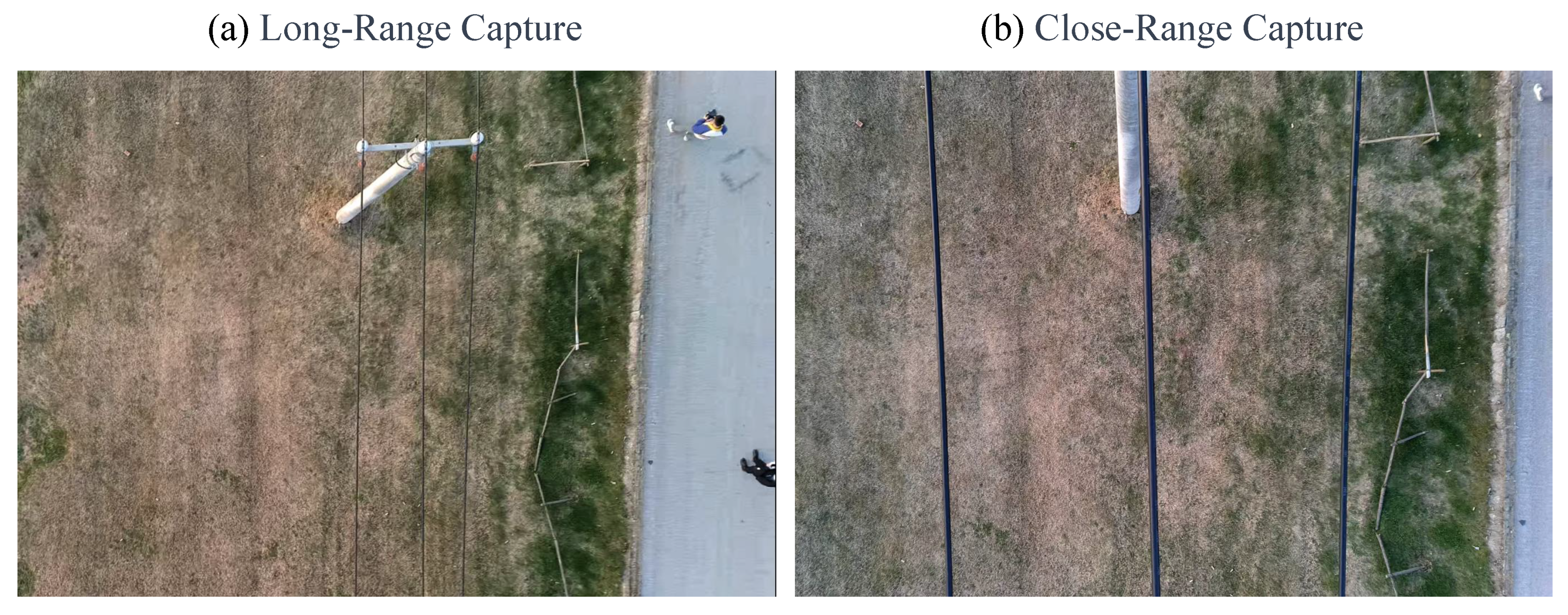
Second, long-range inspection is the most adopted mode regarding inspection type. Long-range inspection can avoid magnetic influence on the sensors used in the platform; moreover, the capture area of the inspection device can be expanded by increasing the distance; hence, the low accuracy problem of the low-cost positioning device can be ignored. However, long-range capture cannot obtain detailed information about the transmission line, as shown in Figure 1.
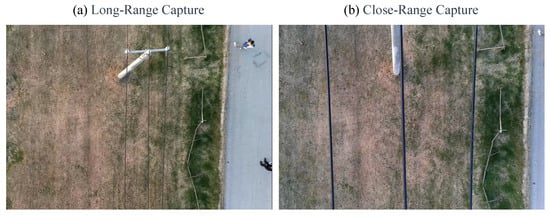
Figure 1.
Captured images of close-range and long-range inspection: (a) capture at 10 m above the transmission line, (b) capture at 2 m above the transmission line.
Figure 1a shows the information of the transmission line captured at long range, where the UAV is kept 10 m away from the transmission line, while (b) is the result of the close-range capture, where the UAV is only 2 m away from the transmission line. The image of the close-range inspection shown in Figure 1b can provide more detailed information, such as checking the transmission line for aging and cracking. Therefore, close-range inspections will be an essential indicator in future transmission line inspection tasks.
Finally, the ability of the UAV to fly along the transmission line has only been partially realized. The UAV should fly along the transmission line to collect complete line information, which requires identifying and detecting the lines. Therefore the identification or detection failure should be addressed; in addition, the wind interference during the flight along the line must be solved.
2.2. System Overview
Based on the above discussion, this work provides a UAV transmission line inspection method using low-cost sensors. The system structure is designed in Figure 2.
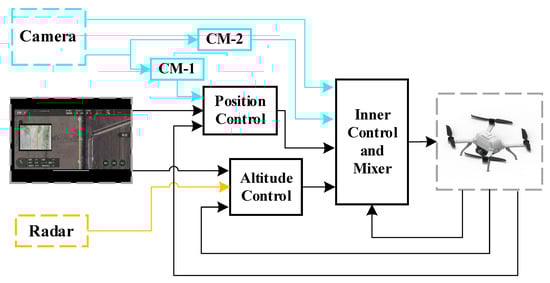
Figure 2.
System structure of transmission line inspection UAV.
In Figure 2, the black line partly depicts the standard cascade structure of the UAV control system, comprising position, altitude, and inner loop controllers. The target trajectory planned in the ground station contains and , corresponding to the position and altitude controllers. The position controller combines the UAV feedback to calculate the inner loop controller’s target (), while the altitude controller outputs thrust T. Finally, the inner loop controller is combined with the feedback to calculate the target rotor speed for each rotor. The additional cameras and mm-wave radar used in the inspection system are indicated by light blue and orange, respectively.
The orange part of Figure 2 shows the mm-wave radar. In addition to being involved in estimating deviation distance , it is mainly involved in the altitude controller as the feedback state during line tracking, thus allowing the UAV to remain at the close range of the transmission line. In addition, the light blue part of the structure indicates how the added cameras act on the system, where relative angle deviation is directly applied to the inner loop controller to correct the UAV’s heading, while is involved in the two CMs. CM-1 is directly applied to the position controller; CM-2 is used to cope with disturbances during line tracking and outputs , the auxiliary roll reference, to participate in the inner loop controller.
With a combination of the two sensors mentioned above, the proposed system is able to track the transmission line at close range. With regard to checks on inspection results, an approach similar to that in [31] is adopted, and the saved HD photos, which were recorded by the camera simultaneously during inspection, are checked by the staff after the inspection is finished.
The following section will present the implementation of the two designed CMs.
3. Transmission Line Position Estimation
3.1. Transmission Line Identification
This section briefly introduces the transmission line identification method based on the Hough transform. Generally, a pre-processing step, such as the grayscale process, grayscale enhancement, filtering, and edge detection, is performed before extracting information from the raw images.
The computational burden is reduced after grayscaling the raw image using the weighted average method, which is highly efficient and computationally quick. Because the grayscale image may lose detailed information, we employed the piecewise linear transformation method to distinguish the specific target and enhance the contrast. An easy-to-implement median filtering method filters out noise generated by the sensors, environments, and transmission. The canny operator is adopted to accurately identify the transmission line edge, which has better anti-interference.
In addition, the extracted edge may accompany interference edges because electric towers are primarily built on highways, fields, and rivers, which serve as noise backgrounds. Therefore, removing the edges generated by the invalid background is necessary after extracting the edges. This process is achieved by masking, which involves ignoring the detection in partial areas.
The entire preprocessing process is shown in Figure 3.
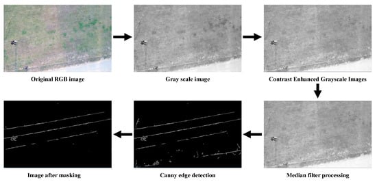
Figure 3.
Pre-processing of raw images.
However, some interference or discontinuity remains in the pre-processed images. Therefore, the Hough transform extracts all the straight lines that meet the threshold, including the target and interference lines. UAV needs to be maintained above the transmission line during inspection, and the line close to the image center is required. Based on the pre-collected images, we draw the following assumptions, which is beneficial in proposing specific rules for convenient line identification.
- The transmission lines from the same tower are made of the same material and have similar characteristics.
- The UAV’s heading should be consistent with the direction of the line; the transmission lines are parallel and share the same direction. In cases of significant direction changes in the transmission line, additional waypoints can be included. This involves dividing the line into multiple directions of unchanged segments for sequential inspection.
- In unique situations, such as tilted cameras, the transmission line may coincide and intersect.
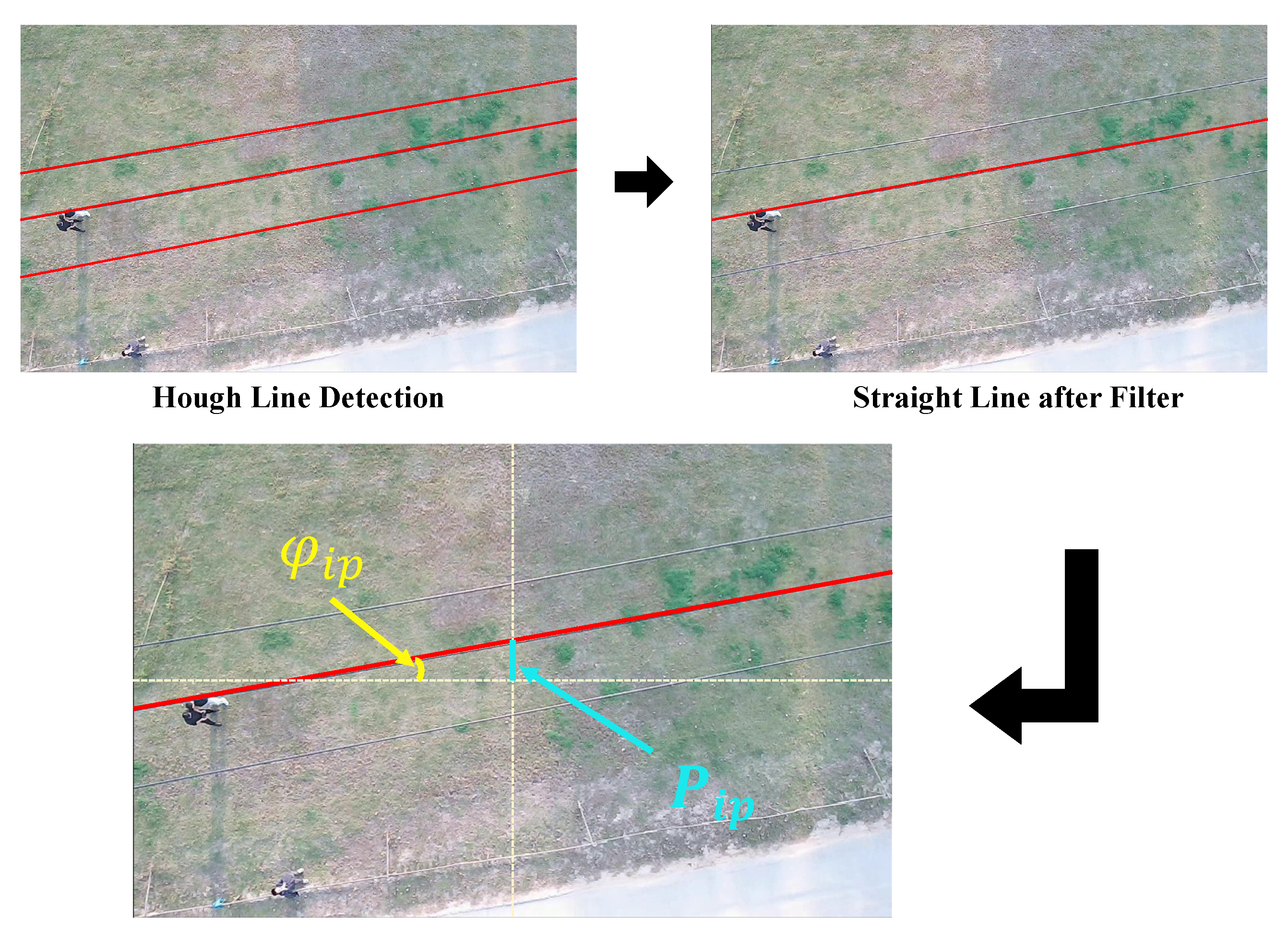
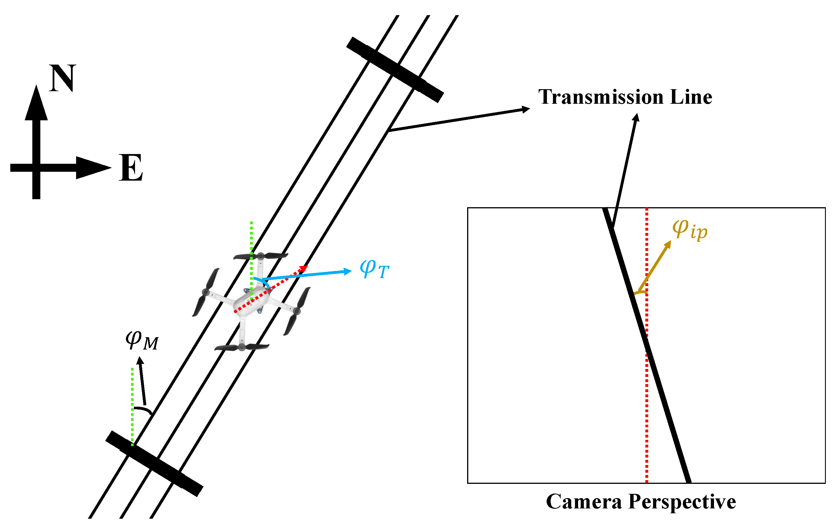
Accordingly, the following selection rule is proposed: First, straight lines whose angle deviation exceeds the threshold are ignored; the remaining lines are then divided based on the angle and grouped into respective sets. Finally, the set with the most significant number is considered as the transmission line set, and the pixel error closest to the image center is regarded as the target line, as shown in Figure 4.

Figure 4.
Illustration of line identification results: The Hough transform detects three lines in the original image, as shown by the red lines in the upper left image. Subsequently, the filter can isolate the desired one. Afterward, the relative information between the target line and the image center can be extracted. represents the angle deviation between the UAV’s heading and the transmission line, while represents the relative pixel distance between them.
3.2. Transmission Line Distance Conversion
In this subsection, along with the mm-wave radar measurements , the process of converting into the standard distance is explained. According to the imaging properties of the camera, the distance between the image distance and object distance satisfies
where is the focal length. According to the principle of pinhole imaging, there is symmetry between the object length , image length , object distance , and image distance , as shown in Equation (2):
The image length can be calculated based on the pixel deviation and unit length . The object distance can be obtained by radar measurement. Then, the actual distance between the transmission line and UAV is
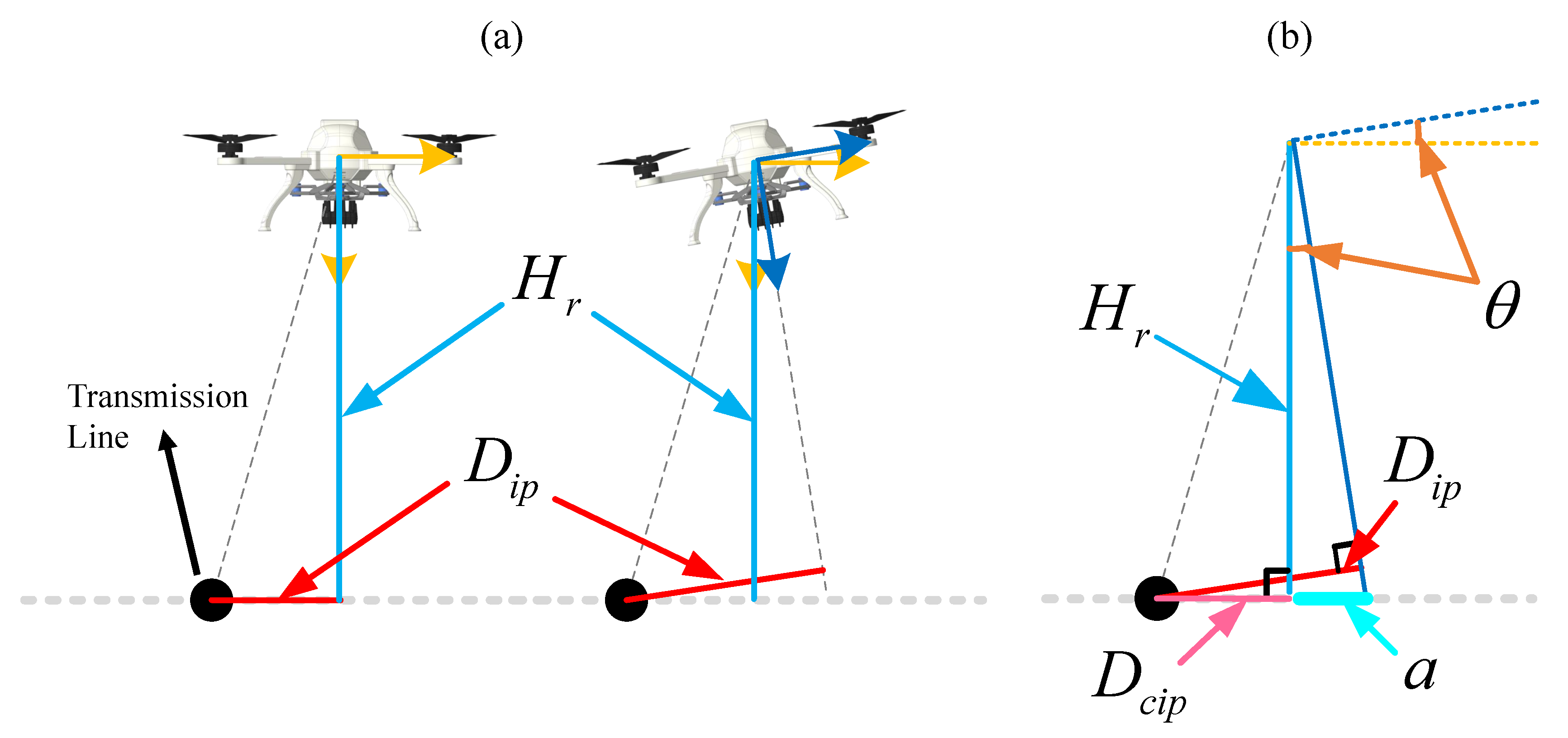
In a typical underactuated system, the motion of the multi-rotor UAV is carried out by adjusting the rotor speed, indicating that the camera fixed to the airframe may be tilted during inspection, as shown in Figure 5a, leading to distorted identification. This problem can be solved using a gimbal; however, the addition of devices implies an increase in cost and the UAV’s weight, which is inconsistent with the design concept of our proposed method. Therefore, we present an attitude compensation solution that combines UAV’s attitude, especially roll (), to process the estimated relative distances. Pitch is not considered since UAV flies forward at a specified velocity during inspection, and thus pitch remains fixed as well; therefore, its impact on the recognition results can be ignored.
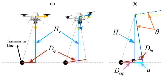
Figure 5.
Identification distortion caused by roll tilt: (a) shows detection distortion caused by tilt, and (b) describes the attitude compensation. represents the vertical distance between UAV and transmission line, is the standard distance calculated following Equation (3) based on and , is the tilt angle of roll, and is the actual relative distance between UAV and transmission line.
With the camera tilted by , the identification results are longer relative to the actual situation, as shown in Figure 5a. For convenience, the relationship between the UAV and transmission line is simplified in Figure 5b.
The auxiliary distance is introduced, and the relationship between the actual distance , auxiliary distance a, and line identification result satisfies Equation (4). Therefore, the actual horizontal distance between the transmission line and UAV can be calculated from Equation (5).
The process described above explains the conversion of pixel of the line identification into the actual distance , using the mm-wave radar and roll of the UAV. However, is performed based on the case where line identification works. How to obtain the horizontal relative distance in the case of abnormal identification needs to be further addressed, which is discussed in Section 3.3.
3.3. Transmission Line Position Estimation
Under normal line identification, indicates the relative distance between the UAV and transmission lines. However, given that there is a significant change in the lighting conditions, or the ground background environment is highly similar to the transmission line, this might lead to identification failure. Therefore, calculating continuous and accurate relative distances can guarantee line-tracking flight.
The results of line identification provide high accuracy but suffer from identification failure, indicating highly accurate but discontinuous signals; in contrast, UAV’s lateral velocity has continuous characteristics but experiences an integral drift problem, which is a constant, relatively low-accuracy signal. Based on the characteristics of these two signals, we propose an adaptive complementary filter in Equation (6) to estimate the relative distance.
represents the estimated relative distance between the transmission line and UAV, k denotes the time series, is the update period of the filter, which depends on the update frequency of line identification, and denotes the lateral velocity of the UAV corresponding to the relative distance. w represents the adaptive factor, updated as follows:
where is the initial weight, and is the positive constant weight. In a desirable situation, 1, which means the recognition result’s variation is consistent with velocity variation. Meanwhile, for the irregular situation, for instances where the UAV’s velocity is distorted or misrecognition occurs during movement, ; thus, the hyperbolic tangent function is selected to constrain such an anomalous result [32]. This design ensures that is involved in the estimation process as a reliable continuous signal, while plays the auxiliary role, ensuring the continuity of the fusion results. adjusts the weight of when detection fails and is a variable related to the reliability of the identification, updated using Equation (8).
updating considers variations in the line identification results. Specifically, when line identification is normal, we evaluate the “velocity” of the relative distance by , and then compare it with . Such rules are formulated to prevent mistaken identification and GNSS velocity anomalies. For example, in the event of misidentification, causing data discontinuity, will be larger than , , will tend to 0, w will be close to the initial , and the weight corresponding to will decrease during fusion; conversely, when line identification is normal and is distorted, w is close to , and the weight corresponding to will be increased. is a small positive constant to prevent singular results.
4. Transmission Line Inspection System
4.1. Heading Correction
During the close-range inspection, the UAV is within the magnetic field of the transmission line, and the compass-measured result differs from the actual situation. However, the UAV’s heading is necessary for autonomous flight. Therefore, the inspection requires an accurate heading to be obtained first.
Since the results of compass measurement are unreliable, the proposed method considered the accurate transmission line’s direction as a reference, and combined it with the image processing results ; thus, the real-time accurate UAV heading can be inverted.
The transmission line’s actual direction can be obtained from the waypoint mission. Generally, the inspection waypoint mission contains the 3D position of the start and endpoints; then, can be computed according to the latitude and longitude of the two points. Although the 3D positions of the start and endpoints in the waypoint mission may deviate from the actual situation, the relative information in the mission is the same as the actual location, suggesting that the direction calculated from the mission points is consistent with the transmission line’s direction. Based on the identification results, the actual heading of the UAV , as shown in Figure 6. Additionally, the case of line identification failure is taken into account: noting that is the heading calculated by the compass, then introducing angular deviation , will be updated if the identification worked. Moreover, when identification fails, will be compensated into . Therefore, the UAV’s actual real-time heading can be obtained by Equation (9).
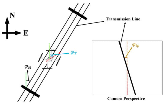
Figure 6.
Illustration of the heading correction: Based on the north direction, which is indicated by the green dotted line, represents the direction of the transmission line calculated based on the waypoint mission; the calculated heading is indicated by the red dotted line, and is the angle deviation provided by line identification; thus, the UAV’s actual heading can be calculated.
4.2. Correction Module 1: Waypoint Correction
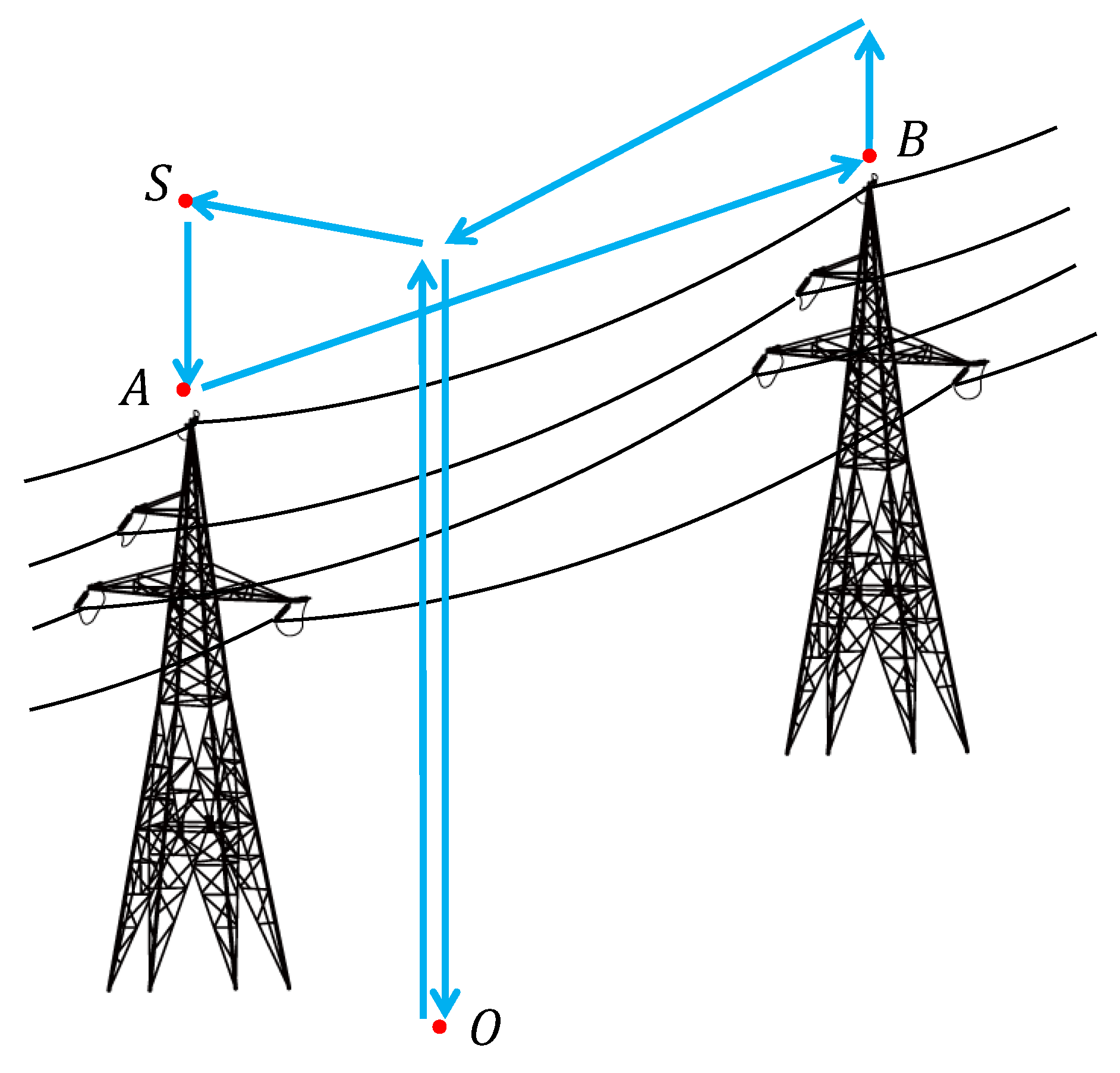
The standard waypoint mission can be planned as follows: UAV takes off from ground O, rises in altitude, reaches auxiliary point S above the transmission line start point A, slowly descends to point A, and, finally, flies directly to the transmission line endpoint B and acquires information during the flight. After reaching point B, which signals the completion of the inspection task, the UAV executes the ’Homing’ instruction and returns to point O. The process is shown in Figure 7.
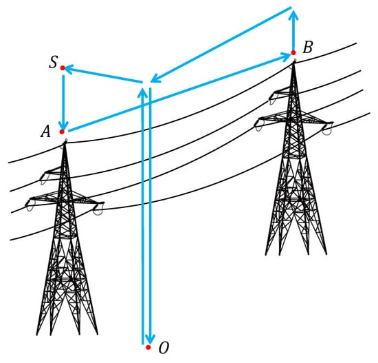
Figure 7.
Illustration of the standard waypoint mission: The UAV takes off from ground O, elevates and moves to the auxiliary point S, which is directly above the mission’s starting point A, then descends to A and flies to the end point B. After reaching B, the UAV returns to the ground O.
However, in practical applications, two undesired situations arise with the standard waypoint missions in Figure 7.
- Case 1: The planned mission trajectory does not match the actual line position. This situation will be further aggravated by the positioning deviation of the UAV’s sensors and the measurement deviation of the start and endpoints of the transmission line.
- Case 2: The UAV flies from A to B without considering external interferences; if the UAV deviates from the trajectory due to wind interference, line information will be lost, leading to incomplete inspection results.
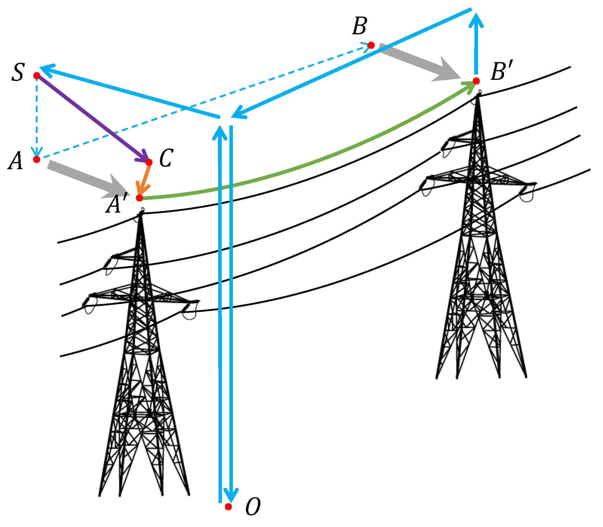
To address case 1, we improved the standard waypoint process and designed CM-1, shown in Figure 8, to address the mismatch problem between the planned and actual position.

Figure 8.
CM-1: Illustration of the improved waypoint mission: 1. Pilot’s initial correction (), C is an arbitrary point close to the actual starting point that can recognize the transmission line, selected by the pilot; 2. Autonomous precision correction (); 3. Mission offset correction (, ), indicates actual end point.)
In the improved waypoint mission, the process from O to S and ‘Homing’ are consistent with the standard waypoint mission. The CM-1 operates from the period the UAV arrives at point S till the end of the mission. At point S, the UAV enters the ‘Manual Operation’ mode, in which the pilot operates the UAV above the actual transmission line’s start point . In contrast to that in [26], this manual process has no strict technical requirements for the staff; however, the acquisition device can recognize the transmission line. Note that the UAV’s current position C is . Combining with , the position of , , can be calculated according to Equation (10).
is the conversion factor between degrees and standard distances, and is the actual transmission line’s position under the current GNSS receiver’s measurement coordinates. Then, the exact position of endpoint under the measurement coordinates can be obtained.
The process described above explains the horizontal coordinate correction in the mission. In contrast, the line-tracking process reflects an aspect different from the standard waypoint, as shown from the green curve in Figure 8. During line tracking, the UAV always maintains a close range to the transmission line, implying vertical position correction during tracking. This process relies on the mm-wave radar.
When the UAV is located at point C, the line identification is valid; simultaneously, will also be recognized as the real-time altitude feedback, and altitude control can be pre-set to a target value; the target will depend on the acquisition capability of the inspection device.
4.3. Correction Module 2: Auxiliary Controller
After the completion of waypoint corrections, the UAV is at point , and the endpoint is corrected to . Under ideal circumstances, the UAV can reach the destination according to the improved trajectory. However, wind disturbance at high altitudes should be addressed, particularly for small UAVs with weak wind resistance. Therefore, the problem of ensuring that UAVs can always fly along the line under wind disturbance remains to be solved. Therefore, we propose CM-2 to alleviate this situation.
The direction of wind interference is random during the along-line flight; however, distinguished by the UAV body coordinates, the headwind (parallel to the UAV heading) is less influential, whereas the crosswind may cause the UAV to be blown off the route. Therefore, an auxiliary controller is added to the inner attitude controller to enhance the anti-wind disturbance capability. The feedback of the auxiliary controller is while the target is at m. Since this controller acts on the UAV sideways, the output of the controller corresponds to , and is superimposed as an additional auxiliary value to the inner roll control.
Considering that it is difficult to model the relationship between the relative distance and roll, the PI algorithm is considered, which does not require a system model and is easier to implement. Note that, if , can be calculated by
where and are the gain coefficients, and is the calculation period. The enhanced autonomous control system is shown in Figure 9. Note that the computation of is independent of the position controller.
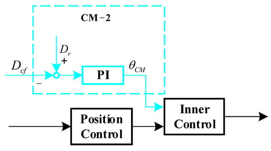
Figure 9.
CM-2: PI-based auxiliary controller. The auxiliary control output is calculated based on the relative distance . is then used as an additional roll target in the inner loop attitude control.
5. Experiment and Verification
5.1. Validation Platform
To validate the practical feasibility of the proposed method, we designed a small-size, low-cost quadcopter UAV, as shown in Figure 10. The UAV is also adaptable to the ground station developed by our team in order to receive the planned trajectory.
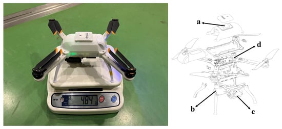
Figure 10.
Independently developed quadcopter inspection UAV. The total weight of 0.484 kg, 0.24 × 0.24 × 0.15 m, mainly consists of a GNSS receiver (a), mm-wave radar (b), RGB camera (c), and main control board (d).
The designed platform has dimensions of 0.24 × 0.24 × 0.15 m, is fitted with a 5-inch propeller, and has a take-off weight of only 0.484 kg; other characteristics of the platform are listed in Table 2. As shown in Figure 10, the platform consists of a GNSS receiver (a), PLK-LC2001l radar (b) [33], OAK-1 RGB camera (c) [34], and main control board (d). The GNSS receiver is mounted on the platform’s top to receive the satellite signals. During inspection, the quadcopter remains above the transmission line; therefore, the mm-wave radar and camera are mounted on the bottom to capture or detect the transmission line. In addition, we removed the shell of the PLK-LC2001l and connected its core board directly to the main control board to reduce weight. The main control board is placed at the center and integrates essential components such as an inertial measurement unit, barometer, compass, and log record module to support autonomous flight.
Table 2.
Quadcopter inspection platform characteristics.
The line identification process is performed in the processor integrated with the camera, while the results of the radar detection are handled within it, before the processed results are sent out. The identification and mm-wave radar detection results are sent to the main control board using the serial port, and the communication frequency is 10 Hz. The main control board adopts a dual Microcontroller Unit (MCU) structure with STM32F4, where the main MCU is used for processing various sensor signals and operating the control system, and the secondary MCU is used for recording the data during flight. The flight control software was developed in the IAR environment [35] using C language. During the running of the quadcopter, the system states and the solutions collected by each sensor are stored in the log record module at 20 Hz.
5.2. Relative Distance Verification
This section examines the proposed line identification and attitude compensation in a static environment. We verify the performance of the proposed adaptive complementary filter with a set of pre-collected data.
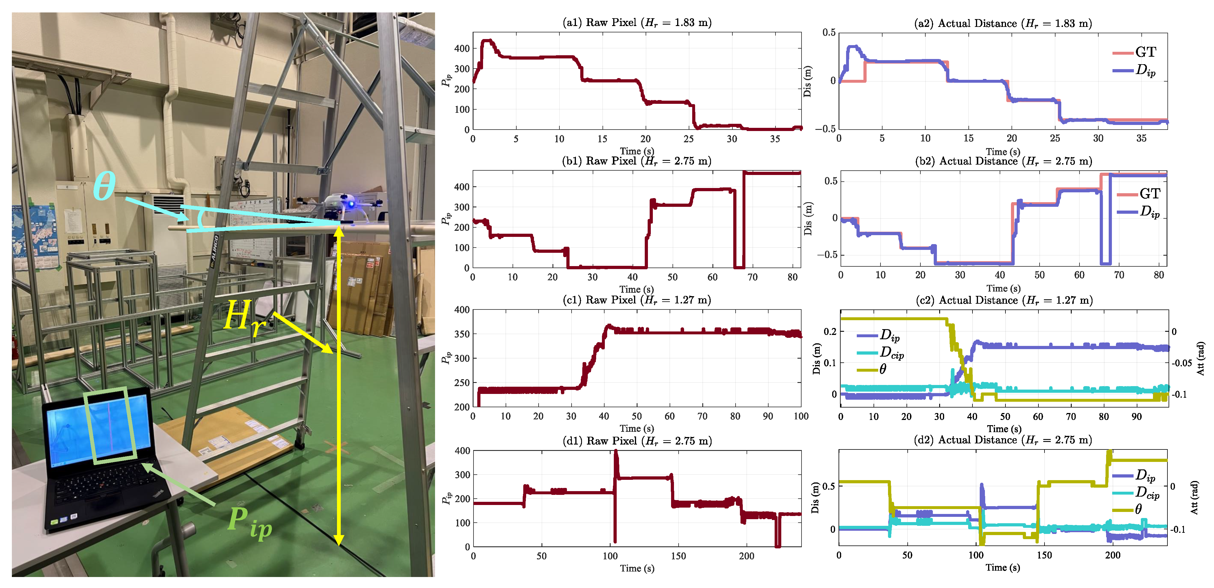
Regarding line identification and attitude compensation, we positioned the quadcopter at a fixed altitude from the ground in the indoor environment. Then, we placed a cable on the ground and moved in the left and right direction at intervals of 0.2 m, with the cable directly below the quadcopter at 0 m. and were recorded during the movement. The parameters of the used camera are = 4.81 mm, and = 1.15 mm. In addition, we adjusted different altitudes and tilts for each experiment. The verification results are shown in Figure 11.

Figure 11.
Static verification of distance identification and attitude compensation. The quadcopter is fixed at the specified altitude with the roll tilt ; then, the cable is moved and the line identification and processing results recorded as (a1,a2) m, rad, (b1,b2) m, rad, (c1,c2) m, rad, and (d1,d2) m, rad.
Figure 11 shows the results of the four experiments. Experiments (a1, a2) and (b1, b2) show the distance estimation of the horizontal situation ( rad) at different altitudes. These two experiments are designed to verify the accuracy of the relative distance calculated in Section 3.2. Experiments (c1, c2) and (d1, d2) explain attitude compensation at different altitudes and tilts.
In experiment a, the quadcopter was placed at 1.83 m; line identification results are shown in Figure 11a1. The identification results change as the cable is moved at 0.2 m intervals. During 5–10 s, the cable was placed 0.2 m to the right of the quadcopter (right lateral direction was defined positive), and the relative distance m, which almost coincides with the ground truth, as represented by the light coral. Similarly, from 13 to 18 s, the cable was moved directly underneath the quadcopter, and m. The pixel acquisition range is 0–480; hence, , indicating that the target object is at the center. Subsequently, in experiment b, we raised the altitude ( m) and moved the cable to the left three times during 0–40 s. is detected as 160, 82, and 2; correspondingly, is −0.206 m, −0.4 m, and −0.612 m, respectively.
For the case where the quadcopter is tilted, at 30–50 s of experiment c, we placed the cable at 0 m and placed the quadcopter at 1.27 m, tilted −0.1 rad, as shown in Figure 11c2, where changed from 0 m to 0.15 m, while remained at 0.008 m. In experiment d, we placed the quadcopter at 2.75 m while adjusting several times. Figure 11d2 shows that the maximum error of with the actual (0 m) is only 0.06 m.
The above four static experiments show the correctness and validity of the relative distance calculation and attitude compensation.
5.3. Adaptive Complementary Filter Verification
We validated the adaptive complementary filter using pre-collected data, as shown in Figure 12. Data collection was conducted in an outdoor environment to obtain the lateral velocity. The cable was placed on the ground, the quadcopter was powered, and line identification was executed; the UAV was laterally swung over the cable, while recording the relevant data, including the relative distance and lateral velocity . During data collection, we masked the camera appropriately to simulate identification failures, as at 11.5–13.9 s and 19.4–21.1 s in Figure 12a.

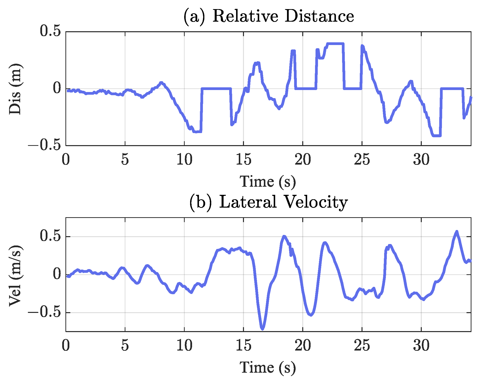
Figure 12.
Pre-collected relative distance and lateral velocity: The adaptive complementary filter is validated using pre-collected data, where the pilot operates the UAV to move laterally above the transmission line, simultaneously recording (a) the detected relative distance , and (b) the lateral velocity .
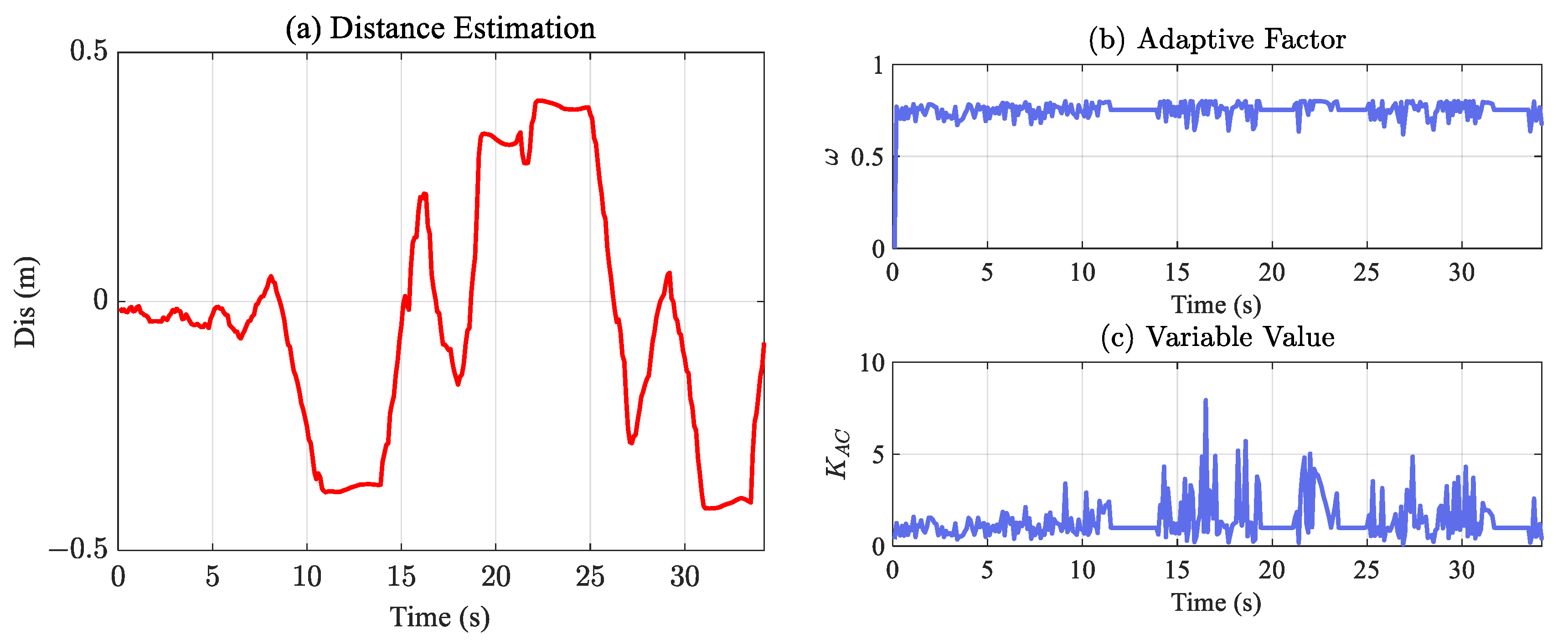
Following Equation (6), we select , , and to fuse the pre-collected data. The results are presented in Figure 13a.

Figure 13.
Adaptive complementary filter results and partial states: The red curve in (a) represents the fusion result , achieved by the proposed filter; in (b) the variation of the adaptive factor w during fusion is depicted, and (c) illustrates the variation of .
Compared to the measured , can better explain distance variation and solve identification failure appropriately. Figure 13b,c present variations in the adaptive factor w and , where w exhibits a variation between 0.2 and 0.6. When outputs more significant results (more than 3), it indicates that the line identification variation is greater than ; moreover, w tends to 0.2, increasing the weight of . In contrast, the weight of increases, which is consistent with the expected design results.
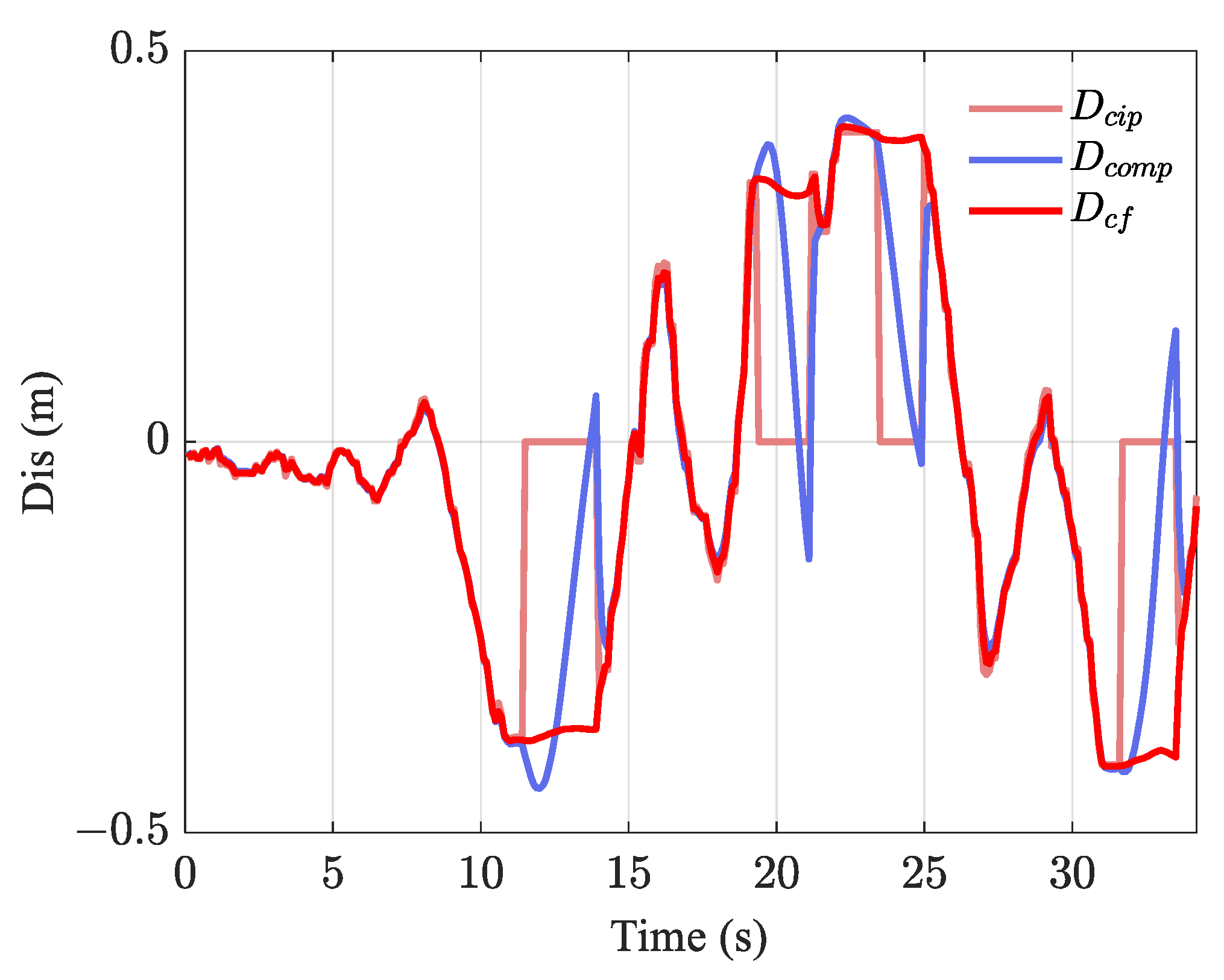
To further reflect the advantages of the proposed adaptive solution, a fixed-parameter complementary filter is similarly implemented for comparison, . The results of the two methods are shown below.
Line identification worked at 14.3–19.1 s, as shown in Figure 14, in which the proposed has better accuracy compared to . There is a significant error between and at 16.1 and 18 s, with a magnitude of 0.04 m. In contrast, almost overlapped with . At 27.3 s, shows a maximum error of 0.07 m with , while that with is only 0.02 m.

Figure 14.
Comparison of different fusion methods for relative distances.
Moreover, when line identification fails, at 11.4–14 s, can be intuitively considered to be inconsistent with the actual situation. However, when line identification recovers at 14 s, m, while m. Similar performance can be found at 21.1, 24.9, and 33.5 s. Compared to the fixed-parameter complementary filter, the designed adaptive complementary filter does not exhibit such a phenomenon, demonstrating the superiority of the proposed adaptive solution.
5.4. Heading Correction Verification
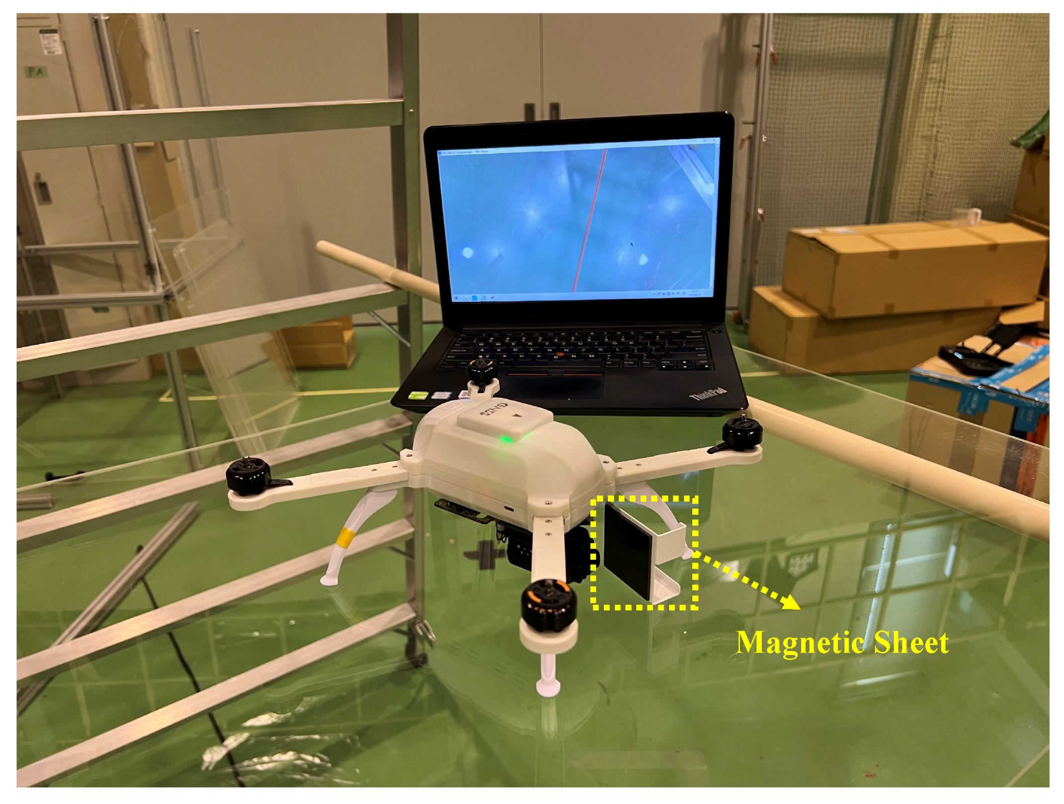
Before actual inspection, the validity of the heading corrections was verified. Under the same environment as that for the relative distance validation, the quadcopter was positioned at a specified altitude, and a cable was placed underneath. The actual direction of the cable was 28 (rotating clockwise from north, 0–360); the quadcopter was put at 1.27 m at 45. A magnetic sheet placed around the quadcopter during the validation process simulated the close-range magnetic interference, as shown in Figure 15. In addition, we simulated anomaly recognition by masking the camera and then recorded compass measurements and state variables related to heading correction.

Figure 15.
Quadcopter in transmission line inspection.
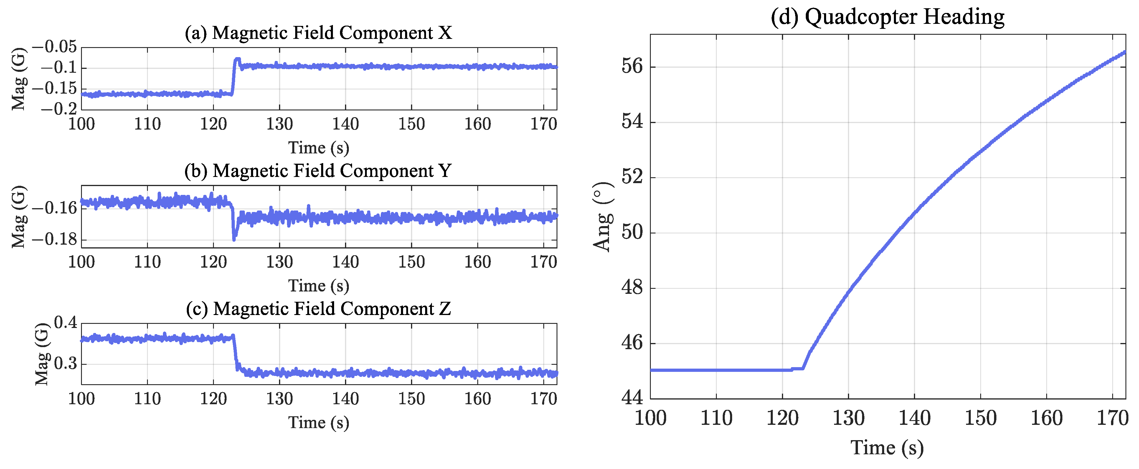
The compass measurements and are displayed in Figure 16, and the magnetic sheet was placed near the quadcopter at 123 s.

Figure 16.
Compass measurements under magnetic interference: (a–c) display the original compass measurements in the X, Y, and Z directions, with magnetic interference introduced at 123 s; (d) illustrates UAV’s heading , calculated based on the compass.
Figure 16a–c show the components of the current magnetic field measured by the compass of each axis under the body coordinate system, while Figure 16d records variations in . With no external interference, the compass accurately calculates the current heading as 45. However, with the magnetic sheet, the magnetic field environment changed significantly, and correspondingly, calculated by relying on the compass measurements continuously drifted by 12 in 48 s. Therefore, during the close-range inspection of the transmission line, the interference caused by the magnetic field should not be ignored. The results of the proposed heading correction are shown in Figure 17.
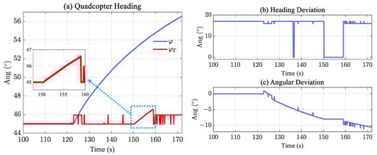
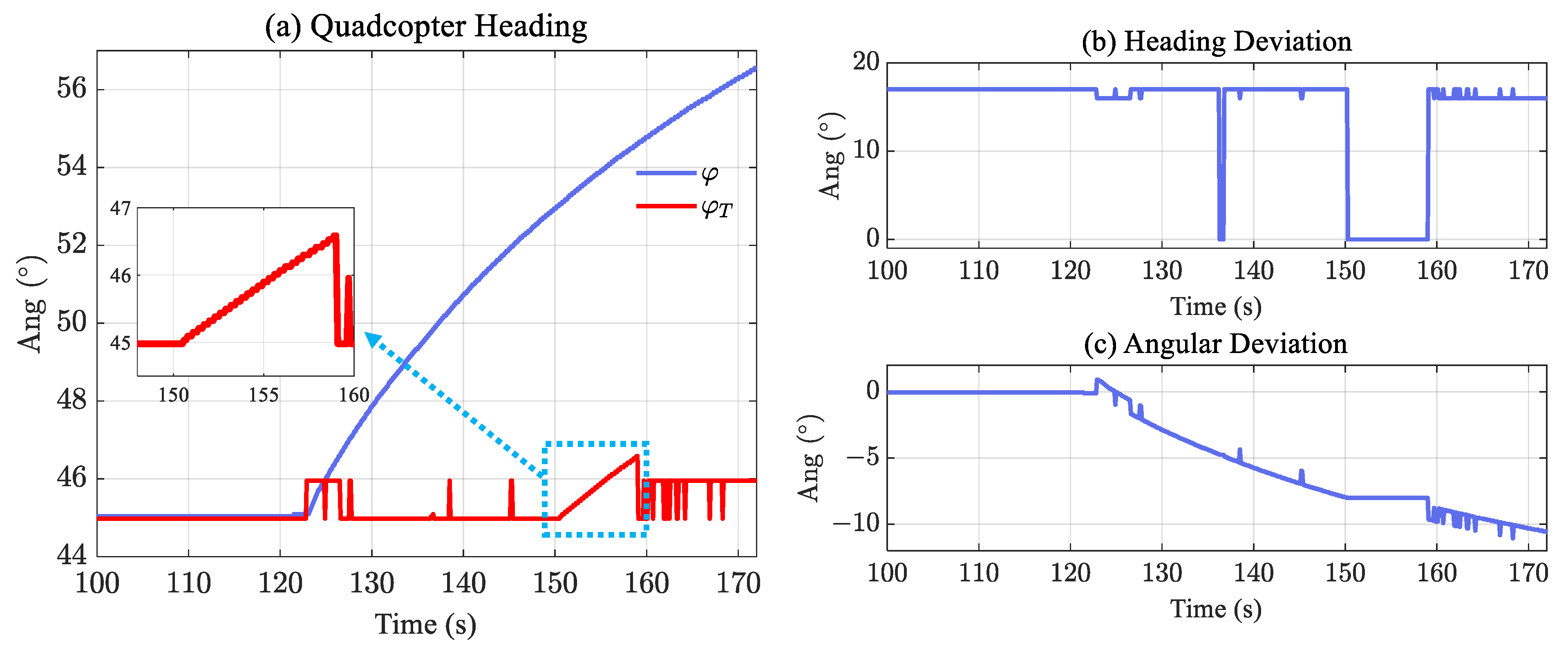
Figure 17.
Validation of heading correction: In the presence of magnetic interference, (a) presents the results of the compass-based calculations alongside the proposed correction results; (b) records the actual heading deviation of the UAV from the transmission line; and (c) shows the variation of the defined angular deviation .
The red curve in Figure 17a shows the compensated heading ; it maintains the actual direction with a maximum error of 2. The recorded in Figure 17b is always maintained at 17, which is consistent with the actual situation. During the line identification work, is constantly updated. In contrast, the identification fails from 150.3 to 159 s, stops updating, and is calculated from and . In the 8.7 s failure period, is also maintained within 2 of the actual situation. Thus, the proposed heading correction can effectively deal with the close-range interference of the transmission line.
5.5. Transmission Line Inspection Application
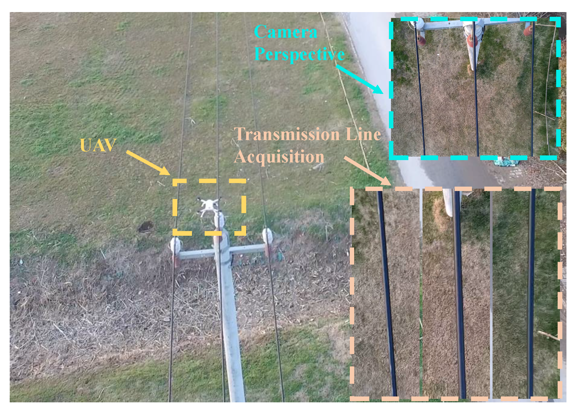
After confirming the critical data, the proposed method was validated according to an actual inspection task using a 10 kV energized transmission line. Following the procedure in Figure 8, the inspection process is executed. First, the standard waypoint mission trajectory is planned at the ground station, the altitude of points A and B is set to 14.1 m (the transmission line altitude is about 12 m), and the distance between the two points is set to 87.9 m. During inspection, it was pre-set to maintain 2 m between the quadcopter and transmission line. In addition, for security reasons, the altitude of the auxiliary point S is set to 25 m. When the quadcopter received the waypoint task, the autonomous ‘Take Off’ instruction was executed and entered the ‘Waypoint Mode’. CM-1 and CM-2 were performed during this process; the RGB camera acquired the HD image of the transmission line. Finally, the quadcopter entered the ‘Homing’ mode automatically. The quadcopter during the inspection and the acquired images are displayed in Figure 18.
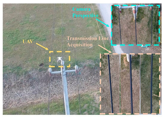
Figure 18.
Quadcopter in transmission line inspection.
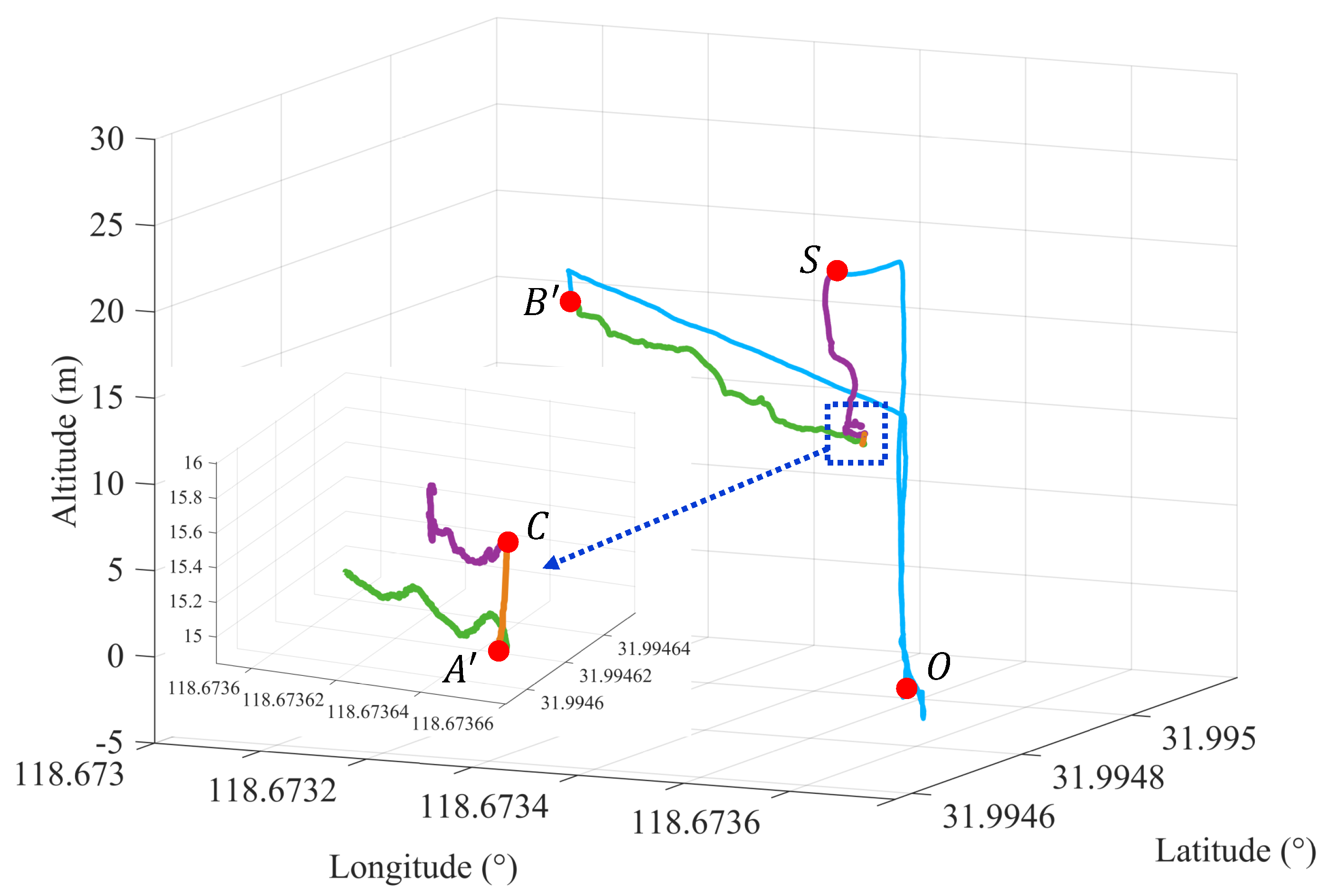
The system states during the inspection process are recorded in the log recording module. The flight trajectory of the quadcopter is shown in Figure 19.
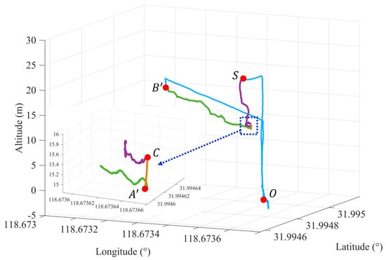
Figure 19.
Flight trajectory of the transmission line inspection: The UAV takes off from the ground and travels to the auxiliary point (, shown in blue), where the pilot operates the UAV for line identification work (, depicted in purple). Subsequently, the UAV flies autonomously over the actual transmission line (, represented in yellow-brown) and begins the inspection (, in green). Finally, the UAV returns to the ground upon completing the mission (, shown in blue).
In Figure 19, the deviation of the mission start point to the actual situation is reflected according to the difference in the horizontal position between the auxiliary point S and actual transmission line start point A, which exemplifies the necessity of the proposed CM-1. After the quadcopter reaches point S, it is operated by the pilot (given by the purple trajectory). Upon reaching the area near the transmission line, where the line identification works, the pilot is no longer operating, and the quadcopter is located at point C; meanwhile, is calculated according to Equation (10) and the endpoint is adjusted to ; the feedback of the altitude control is switched to , and the quadcopter reaches the point directly above the transmission line (the orange line represents this process). The green line represents the line-tracking process, while the quadcopter targets and executes CM-2. Finally, the quadcopter completes the task and executes the ’Homing’ command, as shown by the blue line.
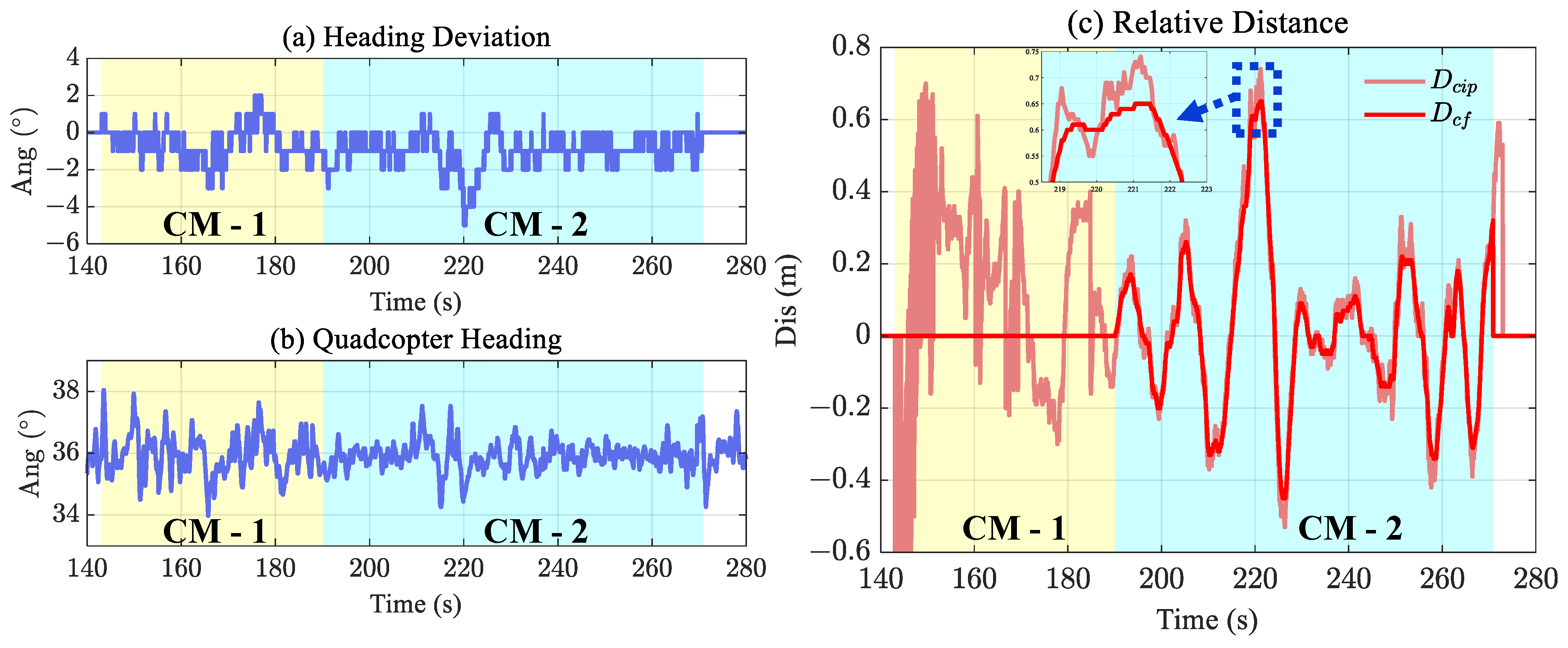
The line identification results are presented in Figure 20. Figure 20a illustrates the angular deviation , which reflects that the quadcopter’s heading was disturbed several times during inspection, at 160–180 s and 212–232 s; notably, reaches a maximum of 5 at 220 s. Figure 20b illustrates , where after compensation, the quadcopter is always maintained at 36, consistent with the actual direction of the transmission line. The relative distances, and , are shown in Figure 20c. is calculated at 190 s, when the quadcopter starts from point . is smoother and avoids abnormal identification compared to , as shown from 218 to 223 s.
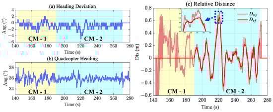
Figure 20.
Distance and heading deviation during inspection: (a) records the heading deviation of identification results; (b) displays the heading calculated by the compass; and (c) illustrates the deviation distance of identification and processed .
During line tracking, the maximum relative distance is 0.72 m, and the transmission line is always within the acquisition range of the camera, proving the proposed CM-2’s effectiveness.
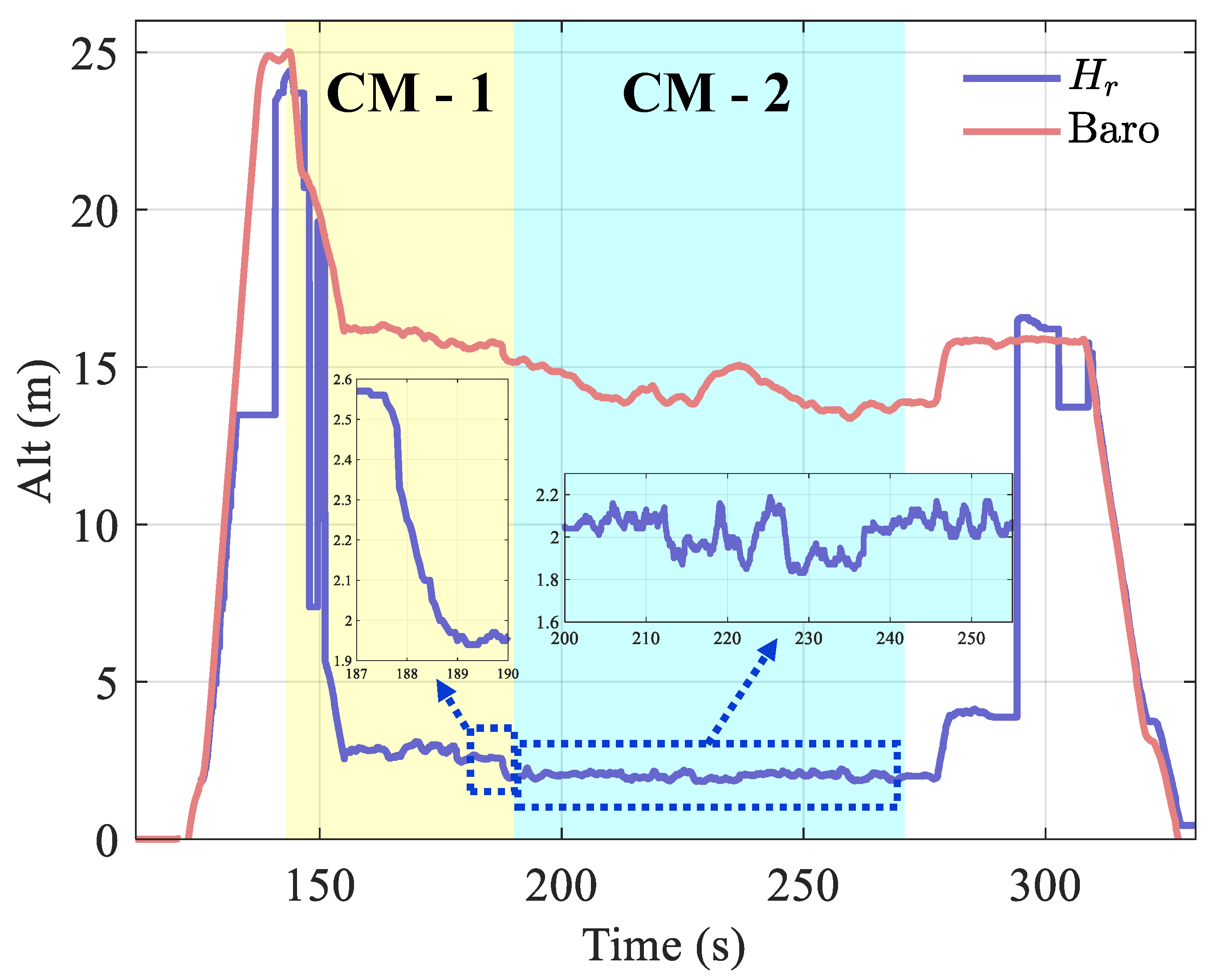
In Figure 21, we present the results of recording the radar and barometer measurements to analyze the quadcopter’s altitude variations.
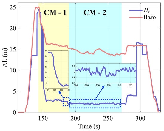
Figure 21.
Altitude during inspection: The dashed line shows the radar measurements during the inspection, which indicate that the UAV remained 2 m above the transmission line, within ±0.2 m error.
In Figure 21, the blue and magenta curves represent the radar trace and barometer measurements, respectively. During 0–139 s, the quadcopter completed take-off and reached the target altitude S. Horizontal position adjustments were then made, reaching S at 143 s. During this period, exhibited detection failure between 132 and 140 s, caused by being outside the measurement range; therefore, we only used the sensor in the transmission line close range, and this situation can be ignored. At 187.5 s, the quadcopter was located at point C; was then controlled to the target at 2 m and maintained throughout the line-tracking process from 190 to 270 s.
Figure 20 and Figure 21 reveal that the quadcopter maintains a close range of 0.65 m horizontally and 2 m vertically with the transmission line during flight, ensuring that the low-cost camera captures the transmission line images. Finally, by checking the photos captured during the inspection, our staff confirmed that the line section we inspected was undamaged.
Thus, the proposed method can be practically applied in transmission line inspection tasks. It is worth mentioning that we only use an RGB camera as the acquisition device as an example; the designed platform can be replaced or different devices added to realize inspection for different purposes. For example, an infrared camera could be added to detect temperature.
6. Conclusions
This work presents a power line inspection method using low-cost sensors, such as GNSS, RGB camera, and mm-wave radar, which collects image information at a close range of the transmission line. Line identification is performed using the knowledge-based Hough transform method. The identified angular deviation is used to cope with the magnetic interference on the compass, while the relative distance between the UAV and transmission line is calculated using the identified pixel deviation. Furthermore, we performed attitude compensation in the relative distance, using an adaptive complementary filter designed to process this distance and enhance the distance estimation robustness. Static and pre-collected data validated the attitude compensation and adaptive filter performance. In addition, we proposed two correction modules to improve the standard waypoint mission. Finally, we designed a small-size quadcopter using low-cost sensors for inspection tasks in a 10 kV energized transmission line environment. The experimental results demonstrate that the proposed method could solve magnetic interference problems for UAV heading, the mismatch between waypoint mission and actual location, and wind interference during line tracking. Therefore, our method offers a valuable reference for the cost-effective and lightweight development of transmission line inspection UAVs, and contributes to promoting the widespread adoption of UAVs for inspection tasks.
However, the line-tracking effect using the proposed method can be further improved, and more advanced control algorithms can be explored to enhance the wind resistance. Moreover, despite using an HD camera and flying within close range of the line, tiny damages are difficult to detect, as are damages on the underneath and side. Therefore, in the future, we will enhance UAV’s wind resistance and increase the variety of targets, such as defects, in the inspection process.
Author Contributions
Conceptualization, Q.W. and S.S.; methodology, Q.W.; software, Q.W. and Z.L.; validation, Q.W. and Z.L.; formal analysis, Q.W.; investigation, Q.W.; resources, Q.W.; writing—original draft preparation, Q.W.; writing—review and editing, W.W., A.N. and S.S. All authors have read and agreed to the published version of the manuscript.
Funding
This research received no external funding.
Data Availability Statement
The data presented in this study are available on request from the corresponding author. The data are not publicly available due to it is obtained using our self-developed platform and is not universal.
Conflicts of Interest
The authors declare no conflict of interest.
Sample Availability
Samples of the compounds are available from the authors.
References
- Katrasnik, J.; Pernus, F.; Likar, B. A survey of mobile robots for distribution power line inspection. IEEE Trans. Power Deliv. 2009, 25, 485–493. [Google Scholar] [CrossRef]
- Takaya, K.; Ohta, H.; Kroumov, V.; Shibayama, K.; Nakamura, M. Development of UAV system for autonomous power line inspection. In Proceedings of the 2019 23rd International Conference on System Theory, Control and Computing (ICSTCC), Sinaia, Romania, 9–11 October 2019; pp. 762–767. [Google Scholar]
- Savva, A.; Zacharia, A.; Makrigiorgis, R.; Anastasiou, A.; Kyrkou, C.; Kolios, P.; Panayiotou, C.; Theocharides, T. ICARUS: Automatic autonomous power infrastructure inspection with UAVs. In Proceedings of the 2021 International Conference on Unmanned Aircraft Systems (ICUAS), Athens, Greece, 15–18 June 2021; pp. 918–926. [Google Scholar]
- Luque-Vega, L.F.; Castillo-Toledo, B.; Loukianov, A.; Gonzalez-Jimenez, L.E. Power line inspection via an unmanned aerial system based on the quadrotor helicopter. In Proceedings of the MELECON 2014—2014 17th IEEE Mediterranean Electrotechnical Conference, Beirut, Lebanon, 13–16 April 2014; pp. 393–397. [Google Scholar]
- Jiang, S.; Jiang, W.; Huang, W.; Yang, L. UAV-based oblique photogrammetry for outdoor data acquisition and offsite visual inspection of transmission line. Remote Sens. 2017, 9, 278. [Google Scholar] [CrossRef]
- Katrasnik, J.; Pernus, F.; Likar, B. New robot for power line inspection. In Proceedings of the 2008 IEEE Conference on Robotics, Automation and Mechatronics, Chengdu, China, 21–24 September 2008; pp. 1195–1200. [Google Scholar]
- Lopez Lopez, R.; Batista Sanchez, M.J.; Perez Jimenez, M.; Arrue, B.C.; Ollero, A. Autonomous uav system for cleaning insulators in power line inspection and maintenance. Sensors 2021, 21, 8488. [Google Scholar] [CrossRef] [PubMed]
- Jenssen, R.; Roverso, D. Automatic autonomous vision-based power line inspection: A review of current status and the potential role of deep learning. Int. J. Electr. Power Energy Syst. 2018, 99, 107–120. [Google Scholar]
- Yang, L.; Fan, J.; Liu, Y.; Li, E.; Peng, J.; Liang, Z. A review on state-of-the-art power line inspection techniques. IEEE Trans. Instrum. Meas. 2020, 69, 9350–9365. [Google Scholar] [CrossRef]
- Zhou, R.; Jiang, W.; Jiang, S. A novel method for high-voltage bundle conductor reconstruction from airborne LiDAR data. Remote Sens. 2018, 10, 2051. [Google Scholar] [CrossRef]
- Zhang, Y.; Yuan, X.; Fang, Y.; Chen, S. UAV low altitude photogrammetry for power line inspection. ISPRS Int. J. Geo-Inf. 2017, 6, 14. [Google Scholar] [CrossRef]
- He, T.; Zeng, Y.; Hu, Z. Research of multi-rotor UAVs detailed autonomous inspection technology of transmission lines based on route planning. IEEE Access 2019, 7, 114955–114965. [Google Scholar] [CrossRef]
- Fang, S.; Haiyang, C.; Sheng, L.; Xiaoyu, W. A framework of power pylon detection for UAV-based power line inspection. In Proceedings of the 2020 IEEE 5th Information Technology and Mechatronics Engineering Conference (ITOEC), Chongqing, China, 12–14 June 2020; pp. 350–357. [Google Scholar]
- Li, H.; Dong, Y.; Liu, Y.; Ai, J. Design and Implementation of UAVs for Bird’s Nest Inspection on Transmission Lines Based on Deep Learning. Drones 2022, 6, 252. [Google Scholar] [CrossRef]
- Yang, T.W.; Yin, H.; Ruan, Q.Q.; Da Han, J.; Qi, J.T.; Yong, Q.; Wang, Z.T.; Sun, Z.Q. Overhead power line detection from UAV video images. In Proceedings of the 2012 19th International Conference on Mechatronics and Machine Vision in Practice (M2VIP), Auckland, New Zealand, 28–30 November 2012; pp. 74–79. [Google Scholar]
- Ballard, D.H. Generalizing the Hough transform to detect arbitrary shapes. Pattern Recognit. 1981, 13, 111–122. [Google Scholar] [CrossRef]
- Zormpas, A.; Moirogiorgou, K.; Kalaitzakis, K.; Plokamakis, G.A.; Partsinevelos, P.; Giakos, G.; Zervakis, M. Power transmission lines inspection using properly equipped unmanned aerial vehicle (UAV). In Proceedings of the 2018 IEEE International Conference on Imaging Systems and Techniques (IST), Krakow, Poland, 16–18 October 2018; pp. 1–5. [Google Scholar]
- Li, Z.; Liu, Y.; Hayward, R.; Zhang, J.; Cai, J. Knowledge-based power line detection for UAV surveillance and inspection systems. In Proceedings of the 2008 23rd International Conference Image and Vision Computing New Zealand, Christchurch, New Zealand, 26–28 November 2008; pp. 1–6. [Google Scholar]
- Tian, F.; Wang, Y.; Zhu, L. Power line recognition and tracking method for UAVs inspection. In Proceedings of the 2015 IEEE International Conference on Information and Automation, Lijiang, China, 8–10 August 2015; pp. 2136–2141. [Google Scholar]
- Zhang, H.; Yang, W.; Yu, H.; Zhang, H.; Xia, G.S. Detecting power lines in UAV images with convolutional features and structured constraints. Remote Sens. 2019, 11, 1342. [Google Scholar] [CrossRef]
- Zhang, J.; Liu, L.; Wang, B.; Chen, X.; Wang, Q.; Zheng, T. High speed automatic power line detection and tracking for a UAV-based inspection. In Proceedings of the 2012 International Conference on Industrial Control and Electronics Engineering, Xi’an, China, 23–25 August 2012; pp. 266–269. [Google Scholar]
- Dietsche, A.; Cioffi, G.; Hidalgo-Carrió, J.; Scaramuzza, D. Powerline tracking with event cameras. In Proceedings of the 2021 IEEE/RSJ International Conference on Intelligent Robots and Systems (IROS), Prague, Czech Republic, 27–30 September 2021. [Google Scholar]
- Kim, S.; Kim, D.; Jeong, S.; Ham, J.W.; Lee, J.K.; Oh, K.Y. Fault diagnosis of power transmission lines using a UAV-mounted smart inspection system. IEEE Access 2020, 8, 149999–150009. [Google Scholar] [CrossRef]
- Cerón, A.; Mondragón, I.; Prieto, F. Onboard visual-based navigation system for power line following with UAV. Int. J. Adv. Robot. Syst. 2018, 13. [Google Scholar] [CrossRef]
- Deng, C.; Liu, J.Y.; Liu, Y.B.; Tan, Y.Y. Real time autonomous transmission line following system for quadrotor helicopters. In Proceedings of the 2016 International Conference on Smart Grid and Clean Energy Technologies (ICSGCE), Chengdu, China, 19–22 October 2016; pp. 61–64. [Google Scholar]
- Mirallès, F.; Hamelin, P.; Lambert, G.; Lavoie, S.; Pouliot, N.; Montfrond, M.; Montambault, S. LineDrone Technology: Landing an unmanned aerial vehicle on a power line. In Proceedings of the 2018 IEEE International Conference on Robotics and Automation (ICRA), Brisbane, Australia, 21–25 May 2018; pp. 6545–6552. [Google Scholar]
- Schofield, O.B.; Iversen, N.; Ebeid, E. Autonomous power line detection and tracking system using UAVs. Microprocess. Microsyst. 2022, 94, 104609. [Google Scholar] [CrossRef]
- Malle, N.H.; Nyboe, F.F.; Ebeid, E.S.M. Onboard Powerline Perception System for UAVs Using mmWave Radar and FPGA-Accelerated Vision. IEEE Access 2022, 10, 113543–113559. [Google Scholar] [CrossRef]
- Peng, X.Y.; Qing, Z.; Rao, Z.Q. Intelligent diagnosis technology for corona discharge defects of transmission lines based on UAV-based UV detection. High Volt. Technol. 2014, 40, 2292–2298. [Google Scholar]
- Guan, H.; Sun, X.; Su, Y.; Hu, T.; Wang, H.; Wang, H.; Guo, Q. UAV-lidar aids automatic intelligent powerline inspection. Int. J. Electr. Power Energy Syst. 2021, 130, 106987. [Google Scholar] [CrossRef]
- Ishino, R.; Tsutsumi, F. Detection system of damaged cables using video obtained from an aerial inspection of transmission lines. In Proceedings of the IEEE Power Engineering Society General Meeting, Denver, CO, USA, 6–10 June 2004; pp. 1857–1862. [Google Scholar]
- Yan, Y.; Zhao, J.; Wang, Z.; Yan, Y. An novel variable step size LMS adaptive filtering algorithm based on hyperbolic tangent function. In Proceedings of the 2010 International Conference on Computer Application and System Modeling (ICCASM 2010), Taiyuan, China, 22–24 October 2010; p. 233. [Google Scholar]
- PLK–LC2001l. 2020. Available online: http://www.plcomp.com/Home/detail.html/3011 (accessed on 21 September 2023).
- OAK–1. 2020. Available online: https://shop.luxonis.com/products/oak-1?variant=42664380334303 (accessed on 21 September 2023).
- IAR. Available online: https://www.iar.com/ (accessed on 21 September 2023).


Disclaimer/Publisher’s Note: The statements, opinions and data contained in all publications are solely those of the individual author(s) and contributor(s) and not of MDPI and/or the editor(s). MDPI and/or the editor(s) disclaim responsibility for any injury to people or property resulting from any ideas, methods, instructions or products referred to in the content. |
© 2023 by the authors. Licensee MDPI, Basel, Switzerland. This article is an open access article distributed under the terms and conditions of the Creative Commons Attribution (CC BY) license (https://creativecommons.org/licenses/by/4.0/).