A Multi-Domain Joint Novel Method for ISAR Imaging of Multi-Ship Targets

Abstract

As a key object on the ocean, regulating civilian and military ship targets more effectively is a very important part of maintaining maritime security. One of the ways to obtain high-resolution images of ship targets is the inverse synthetic aperture radar (ISAR) imaging technique. However, in the actual ISAR imaging process, ship targets in a formation often lead to complicated motion conditions. Due to the close distance between the ship targets, the rough imaging results of the targets cannot be completely separated in the image domain, and the small differences in motion parameters lead to overlapping phenomena in the Doppler history. Therefore, for situations in which ship formation targets with little difference in motion parameters are included in the same radar beam, this paper proposes a multi-domain joint ISAR separation imaging method for multi-ship targets. First, the method performs echo separation using the Hough transform (HT) with the minimum entropy autofocus method in the image domain. Secondly, the time–frequency curve is extracted in the time–frequency domain using the short-time Fourier transform (STFT) for time–frequency analysis, which solves the problem of the ship formation targets being aliased on both echo and Doppler history after range compression and achieves the purpose of separating the echo signals of the sub-ship targets with high accuracy. Eventually, better-focused images of each target are obtained via further motion compensation and precise imaging. Finally, the effectiveness of the proposed method is verified using a simulation and measured data.

1. Introduction

The synthetic aperture radar (SAR) plays a significant role in various fields, including land and resources, earthquake, mapping, environment, disaster monitoring, and forestry [1]. Additionally, the inverse synthetic aperture radar (ISAR) is a radar imaging system capable of acquiring high-resolution images of moving targets [2,3,4,5,6,7]. Parameter estimation and motion compensation are key techniques in ISAR imaging [8,9]. When a high-resolution radar is applied to multi-target imaging, such as ship target formations, multi-targets will likely appear in the same radar beam. For the sake of convenient description, individual targets in a formation are defined as sub-targets. When a sub-target moves in closely, their echoes overlap in the range-slow time domain. In this case, the correlation between adjacent echoes will be low, leading to the failure of traditional motion compensation methods [10,11,12,13,14,15,16] and thus increasing the difficulty of accurate sub-target discrimination and imaging. Currently, imaging of multi-targets moving within the same radar antenna beam has received extensive attention from many scholars.

In recent years, research on ISAR imaging techniques for multiple targets has yielded many results. There are two main solutions: multi-target direct imaging and multi-target separation imaging. Among them, multi-target separation imaging can also be specifically categorized into multi-target image domain separation, multi-target signal domain separation, and multi-target parameter domain separation [17,18,19]. For direct multi-target imaging, most existing methods are realized via range-instantaneous Doppler [20,21] imaging techniques based on time–frequency analysis. Zhaoda Zhu [22] and Jiawei Wu [23] viewed a multi-target as a rigid whole target for unified motion compensation, then used time–frequency analysis in the time–frequency domain to extract the target curves presenting different Doppler time-varying characteristics, and finally inverted the time–frequency transformation of the multi-target to the echo domain for the next imaging process. V. C. Chen et al. similarly subjected the multi-target as a whole to motion compensation and then used the joint time–frequency transform to image the multi-target instantaneously [24]. However, when the range cell contains many scatterers or a multi-target with similar motion states, the above methods will encounter problems such as cross terms and low resolution. J. Chen et al. realized ISAR multi-target simultaneous imaging using the Sandglass transform and finally obtained well-focused multi-target ISAR imaging results with peak projection [25].

For multi-target image domain separation imaging, Jun Yang et al. used the target motion parameters obtained from the narrowband radar to compensate the broadband signal for motion, and its performance depends on the accuracy of the narrowband radar data to estimate the target velocity [26]. Wenchi Chen et al. utilized the Keystone transform simultaneously to compensate for the target’s translational velocity component [27]. S. H. Park et al. utilized the Hough transform (HT) to detect the slope of the range profile of a multi-target, after which they constructed a mask based on the slopes to separate each target’s range profile, which was finally processed separately using the ISAR imaging method [28]. Later, S. H. Park et al. focused their research on motion compensation prior to rough imaging with better imaging results [29]. However, the above methods cannot effectively distinguish between multi-targets when their echoes cross heavily after range compression. Xueru Bai et al. [30] proposed a formation imaging method for uniform linear motion and obtained well-focused multi-target images by finely compensating the second-order and third-order phase terms. Currently, most of the multi-target imaging methods based on image domain separation apply to situations where the difference in motion states between sub-targets is not large.

Many multi-target signal-domain separation and multi-target parameter-domain separation imaging methods have been proposed based on the existence of differences in motion parameters between sub-targets. Zhaoda Zhu et al. used the maximum likelihood estimation method to estimate the sub-target motion parameters and compensated imaging based on the motion parameters [31,32]. The prerequisite of the method is that there is no relative motion between the targets, which limits its applications in reality. V. C. Chen et al. used the Doppler histories of different targets to separate the targets, and this method works well when the targets have significant acceleration differences, but when the accelerations are similar, the separation effect is more general [33,34]. Wenchi Chen utilizes discrete frequency modulated Fourier transform for parameter estimation and separates the sub-target signals from the echoes before further processing [35]. J. Chen et al. transformed the problem of separating multi-target echoes into estimating the frequency modulation rate of multi-component linear frequency modulated (LFM) signals and then used Gaussian short-time fractional-order Fourier transform to estimate the frequency modulation rate of the sub-target echoes to realize the echo separation [36]. Xiao Dong et al. proposed a multi-target ISAR imaging method based on sparse representation, but the imaging performance of this type of method degrades when there is severe coupling between sub-target echoes [37]. Dong Zhang et al. utilized a time–frequency transformation method to estimate the motion parameters of different targets to accomplish separated imaging [38]. All the above multi-target imaging algorithms have their advantages and disadvantages, but in general, they have limitations.

This paper proposes a multi-domain joint ISAR separation imaging method for multi-ship targets for situations in which ship formation targets with little difference in motion parameters are included in the same radar beam. The fine focusing of the ship target is accomplished by two separations in the image and time–frequency domains using HT and time–frequency analysis techniques, respectively. Compared to traditional image domain separation imaging methods, traditional image domain separation methods are susceptible to factors such as noise and interference, leading to incomplete separation of sub-targets and resulting in blurry or distorted imaging results. The method proposed in this paper, through signal analysis and processing, can accurately capture the characteristics of sub-targets and precisely separate their echo data, thereby providing clearer and more accurate imaging results. Finally, the effectiveness of the method proposed in this paper is verified via simulation and measured data.

This paper is organized as follows. Section 2 describes the geometric model and signal model of multi-ship targets. Section 3 describes the joint multi-domain ISAR separation imaging method for multi-ship targets. Section 4 verifies the effectiveness of the proposed method through experiments. Finally, Section 5 summarizes the whole paper.

2. ISAR Imaging Geometry and Signal Model

2.1. Multi-Target ISAR Echo Signal

Taking a ship target as an example, multi-target ISAR imaging in the imaging accumulation time, the radar carrier for speed $v_a$, height $H_a$ for uniform linear motion and the radar line of sight (RLOS) within the continuous irradiation of $Q$ targets, each target has its state of translation and rotation. Consider each target as a collection of a series of scattering points, e.g., assume that the $q\left(q=1,\dots ,Q\right)$th target contains $K_q$ scattering points. The geometric model of multi-target motion is shown in Figure 1.

Assume that the ISAR radar transmits a LFM signal [39,40], which is

$$s\left(t\right)=\mathrm{rect}\left(\frac{t}{T_p}\right)\exp \left[j2\pi \left(f_{c}t+\frac{1}{2}\gamma t^2\right)\right]$$

(1)

where $\mathrm{rect}(·)$ denotes the rectangular window function, $t$ represents the fast time, $T_p$ represents the signal pulse width, $f_c$ denotes the signal carrier frequency, and $\gamma$ represents the signal frequency modulation rate, $\gamma =B/T_p$. If the $k\left(k=1,\dots K_q\right)$th scatterer of the target $q$ has an instantaneous distance from the radar at time $t_m$ as $R_{q,k}\left(t\right)$, the echo signal can be represented as

$$\begin{array}{ll}{S}_r\left(t,t_m\right)& ={{\displaystyle \sum }}_{q=1}^Q{{\displaystyle \sum }}_{k=1}^{K_q}\{{\sigma }_{k,q}\mathrm{rect}\left[\frac{\left(t-\frac{2R_{q,k}\left(t_m\right)}{c}\right)}{T_p}\right]\\ & ·\exp \left(j2\pi \left[f_c\left(t-\frac{2R_{q,k}\left(t_m\right)}{c}\right)+\frac{1}{2}\gamma {\left(t-\frac{2R_{q,k}\left(t_m\right)}{c}\right)}^2\right]\right)\}\end{array}$$

(2)

where ${\sigma }_{k,q}$ represents the backscattering coefficient of the $k$th scatterer of the target $q$.

After de-chirp processing, the difference frequency signal can be expressed as

$$s_{if}\left(t,t_m\right)={{\displaystyle \sum }}_{q=1}^Q{{\displaystyle \sum }}_{k=1}^{K_q}\left\{{\sigma }_{k,q}\mathrm{rect}\left[\frac{\left(t-\frac{2R_{q,k}\left(t_m\right)}{c}\right)}{T_p}\right]\cdot {\exp }^{-j\frac{4\pi }{c}\left(\gamma \left(\widehat{t}-\frac{2R_{ref}}{c}\right)+f_c\right)R_{\Delta }}\right\}$$

(3)

where $R_{\Delta }=R_{q,k}\left(t\right)-R_{ref}$, $R_{ref}$ is the reference distance. By applying the Fourier transform in the fast time domain to Equation (3), the following equation can be obtained:

$$S_{if}\left(f_i,t_m\right)={{\displaystyle \sum }}_{q=1}^Q{{\displaystyle \sum }}_{k=1}^{K_q}\left\{{\sigma }_{k,q}{T}_{p}sinc\left[T_p\left(f_i+2\frac{\gamma }{c}{R}_{\Delta }\right)\right]\exp \left(-j\frac{4\pi }{c}{f}_c{R}_{\Delta }\right)\right\}$$

(4)

where ${\sigma }_{k,q}{T}_{p}sinc\left[T_p\left(f_i+2\frac{\gamma }{c}{R}_{\Delta }\right)\right]$ represents the $\sin \mathrm{c}$ envelope of a single scatterer on the echo after range compression, and it can be seen that $R_{\Delta }$ causes a translation of the envelope with a slow time change. However, due to the different $R_{q,k}\left(t\right)$ changes of different targets, the correlation between adjacent envelopes is reduced, which makes the traditional motion compensation method unusable in multi-target imaging.

2.2. Principle of Multi-Target ISAR Echo Separation

Still taking the ship target as an example, $R_{\Delta }$ in Equation (4) should contain the translation component and the rotation component of the target so that it can be further expressed as

$$\Delta R_{q,k}\left(t\right)=R_q\left(t\right)+ysin\left({\theta }_q\left(t\right)-\alpha \right)-xcos\left({\theta }_q\left(t\right)-\alpha \right).$$

(5)

Thus, the phase of the $k$th target echo signal can be obtained as

$${\Phi }_q\left(r_t\right)=\frac{4\pi f_c}{c}\left[R_k\left(t\right)-ysin\left({\theta }_k\left(t\right)-\alpha \right)+xcos\left({\theta }_k\left(t\right)-\alpha \right)\right]$$

(6)

The time differential of Formula (6) can be used to obtain the Doppler frequency shift caused by target motion.

$$\begin{array}{ll}{f}_{D_k}& =\frac{2f_c}{c}{V}_{R,k}+\frac{2f_c}{c}\frac{d}{dt}\left[x\mathit{cos}\left({\theta }_{0,k}+{\Omega }_{k}t-\alpha \right)-y\mathit{sin}\left({\theta }_{0,k}+{\Omega }_{k}t-\alpha \right)\right]\\ & =\frac{2f_c}{c}{V}_{R,k}+\frac{2f_c}{c}\left[-x{\Omega }_k\mathit{sin}\left({\theta }_{0,k}+{\Omega }_{k}t-\alpha \right)-y{\Omega }_k\mathit{cos}\left({\theta }_{0,k}+{\Omega }_{k}t-\alpha \right)\right]\\ & =\frac{2f_c}{c}{V}_{R,k}+\frac{2f_c}{c}\left\{-x{\Omega }_k\left[\mathit{sin}\left({\theta }_{0,k}-\alpha \right){\mathit{cos}\Omega }_{k}t+\mathit{cos}\left({\theta }_{0,k}-\alpha \right){\mathit{sin}\Omega }_{k}t\right]\right.\\ & \left.-y{\Omega }_k\left[\mathit{cos}\left({\theta }_{0,k}-\alpha \right){\mathit{cos}\Omega }_{k}t-\mathit{sin}\left({\theta }_{0,k}-\alpha \right){\mathit{sin}\Omega }_{k}t\right]\right\}\end{array}$$

(7)

where $V_{R,k}$, ${\theta }_{0,k}$, and ${\Omega }_k$, respectively, represent the initial velocity, initial rotation angle, and rotation angular rate of the target $k$, and the above formula only gives the zero-order term and the first-order term. For a given rotation angular rate and coherent processing time $t$, if ${\Omega }^2{t}^2\ll 1$ and ${\Omega }^3{t}^3\ll \Omega t$, then

$$cos\Omega t=1-{\Omega }^2{t}^2/2+\cdots \cong 1.$$

(8)

$$sin\Omega t-{\Omega }^3{t}^3+\cdots \cong \Omega t$$

(9)

Therefore, it is possible to obtain

$$\begin{array}{ll}{f}_{D_k}& =\frac{2f_c}{c}{V}_{R,k}+\frac{2f_c}{c}\left\{-x{\Omega }_k\left[\mathit{sin}\left({\theta }_{0,k}-\alpha \right)+\mathit{cos}\left({\theta }_{0,k}-\alpha \right){\Omega }_{k}t\right]\right.\\ & \left.-y{\Omega }_k\left[\mathit{cos}\left({\theta }_{0,k}-\alpha \right)-\mathit{sin}\left({\theta }_{0,k}-\alpha \right){\Omega }_{k}t\right]\right\}\\ & =\frac{2f_c}{c}{V}_{R,k}+\frac{2f_c}{c}\left\{-\left[x\mathit{sin}\left({\theta }_{0,k}-\alpha \right)+y\mathit{cos}\left({\theta }_{0,k}-\alpha \right)\right]{\Omega }_k\right.\\ & \left.-\left[x\mathit{cos}\left({\theta }_{0,k}-\alpha \right)-y\mathit{sin}\left({\theta }_{0,k}-\alpha \right)\right]{\Omega }_k^{2}t\right\}\\ & =f_{D_{T,k}}+f_{D_{\mathrm{R},\mathrm{k}}}.\end{array}$$

(10)

Therefore, the Doppler shift due to translational motion is

$$f_{D_{T,k}}=\frac{2f_c}{c}{V}_{R,k}$$

(11)

The Doppler shift due to rotational motion is

$$\begin{array}{ll}{f}_{D_{R,k}}& =\frac{2f_c}{c}\{-\left[xsin\left({\theta }_{0,k}-\alpha \right)+ycos\left({\theta }_{0,k}-\alpha \right)\right]{\Omega }_k\\ & -\left[xcos\left({\theta }_{0,k}-\alpha \right)-ysin\left({\theta }_{0,k}-\alpha \right){\Omega }_k^{2}t\right]\}.\end{array}$$

(12)

When $V_{R,k}$ and ${\Omega }_k$ are constants, the Doppler shift is still time-varying because the

$$\frac{d}{dt}{f}_{D_k}=\frac{2f_c}{c}\left[-x^2{\Omega }_k^{2}cos\left({\theta }_{0,k}-\alpha \right)+ysin\left({\theta }_{0,k}-\alpha \right)\right].$$

(13)

From Equation (13), although multi-targets cannot be discriminated in the range due to the different Doppler shifts and rates of change, the estimation method of multi-component LMS can still be used from the perspective of the signal domain, such as discrete chirp Fourier transform (DCFT) [41], adaptive wavelet basis decomposition [42], and Randon transform (RT) [43,44,45] to estimate the acceleration influence term of different targets and separate different target signals.

From Equation (6), when the target shows uniform motion, the range compression echo is reflected as several slanted lines with a certain slope and width. Since the radial speeds of the targets are different, the slopes of the corresponding slopes are also different, which is manifested as a divisible or partial cross in the echo. Therefore, it is also possible to start from the image domain, estimate the slope of a slanted line using the method of slanted line detection, construct a mask to separate the echoes of sub-targets one by one, and then utilize the single-target ISAR imaging method to complete the processing for each target separately. When the target makes a complex movement, the echo after range compression cannot be treated as a slanted line. Therefore, it is first necessary to preprocess using specific range migration correction methods, such as HT, generalized Keystone transform [46], and so on.

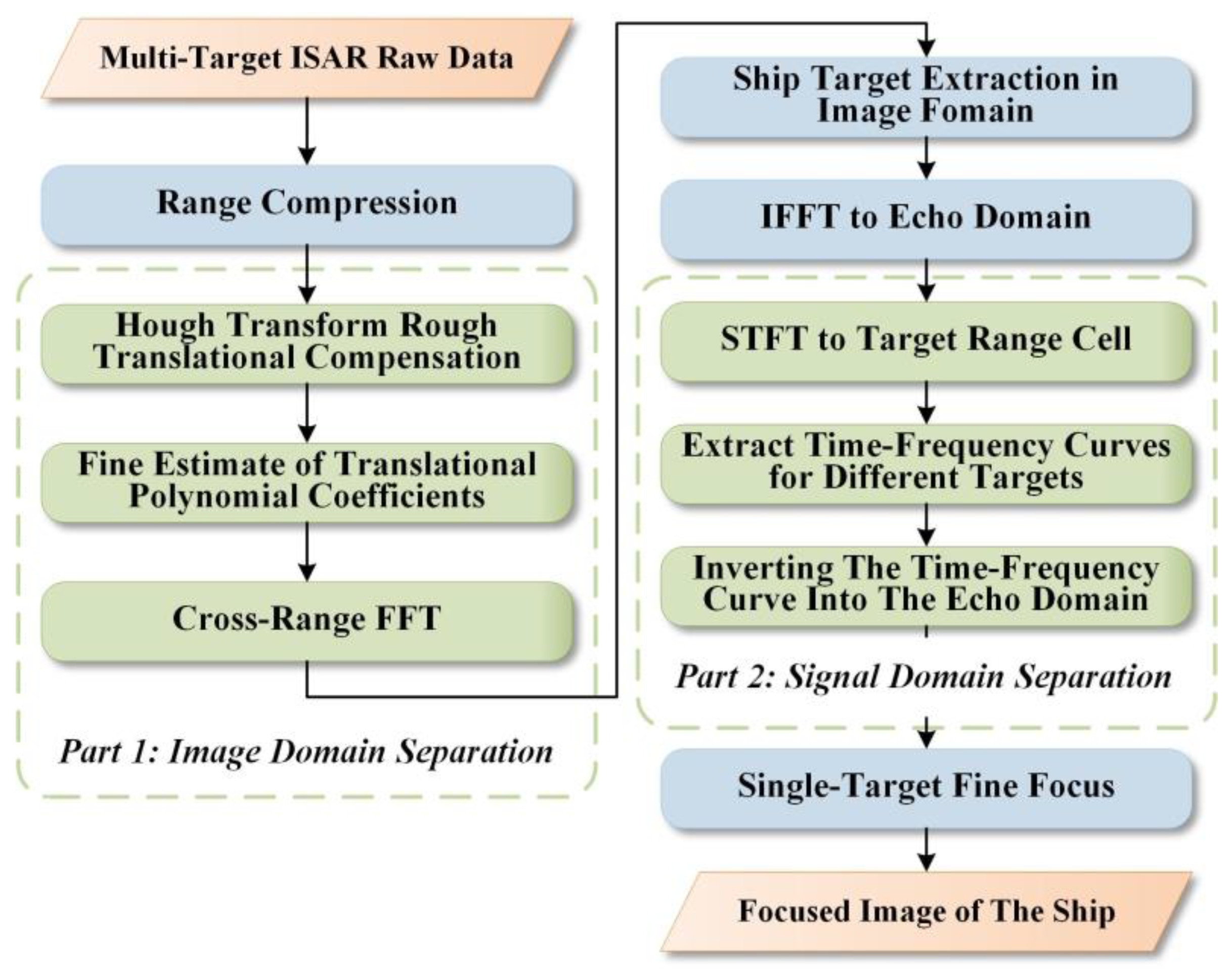
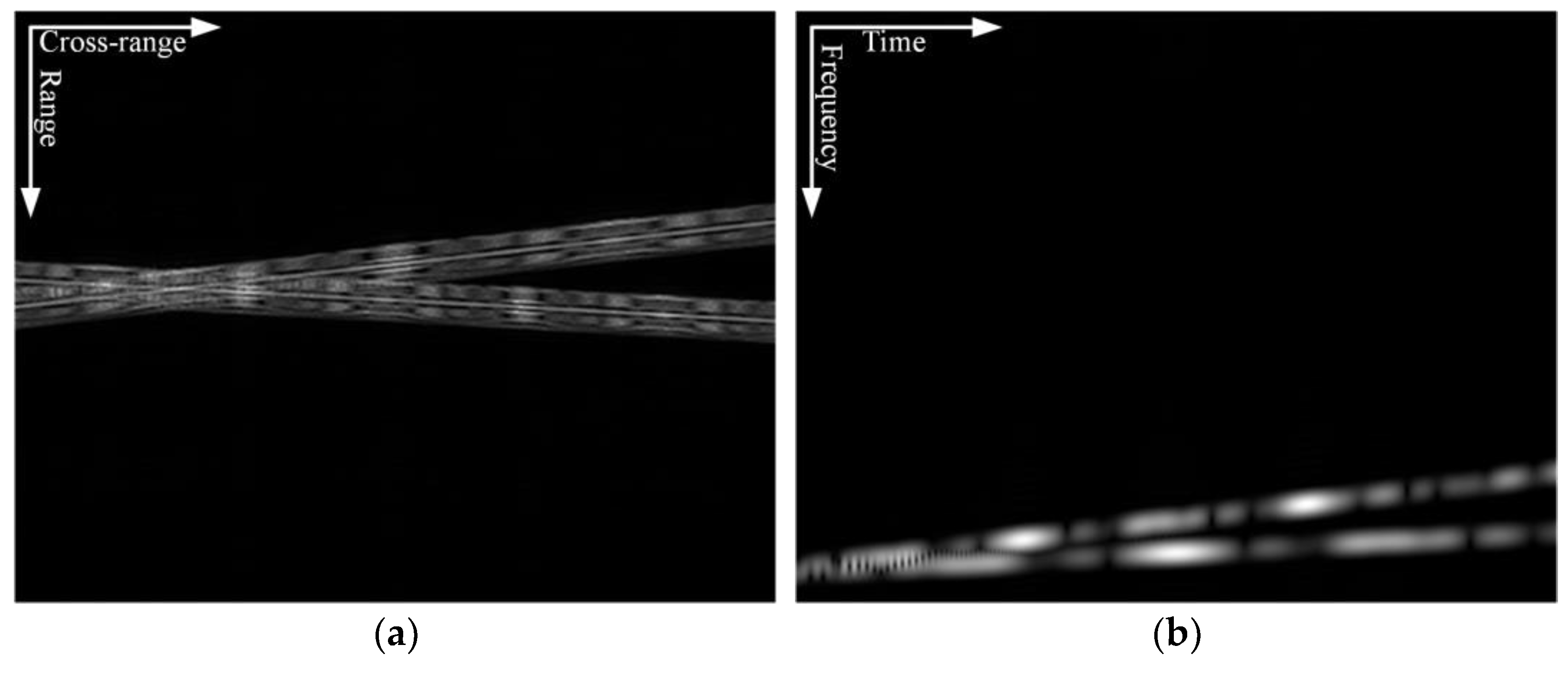
3. Multi-Ship Target ISAR Imaging Method Based on HT and STFT

To solve the problem of imaging ship formation targets that contain little difference in motion parameters within the same radar beam, this paper proposes an echo separation method applicable to ship formation imaging, which mainly has two key steps. First, the HT is used to compensate for the translational parameters initially, followed by rough imaging and inverting the ship target back to the data domain. Secondly, STFT is used for time–frequency analysis of the target, and secondary separation is performed in the time–frequency domain. Finally, fine focusing is accomplished using a single-target motion compensation method. The complete flowchart of the proposed method is shown in Figure 2.

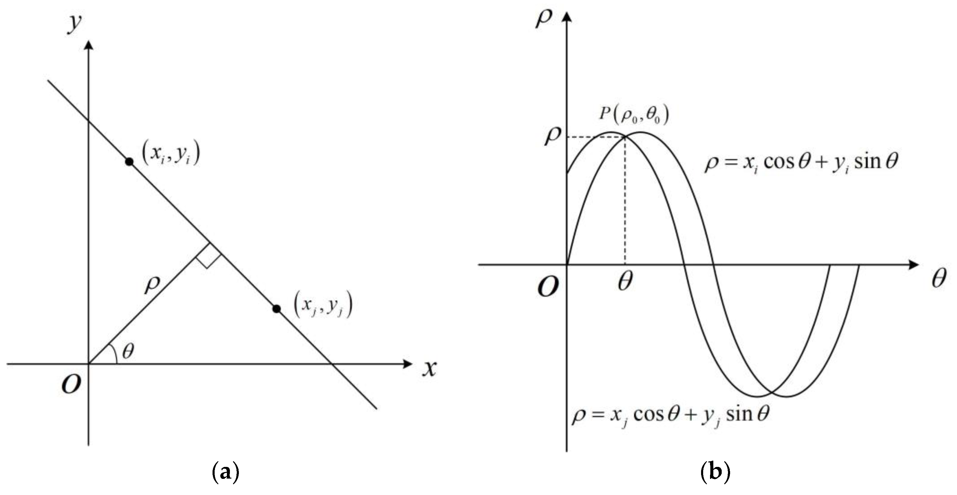
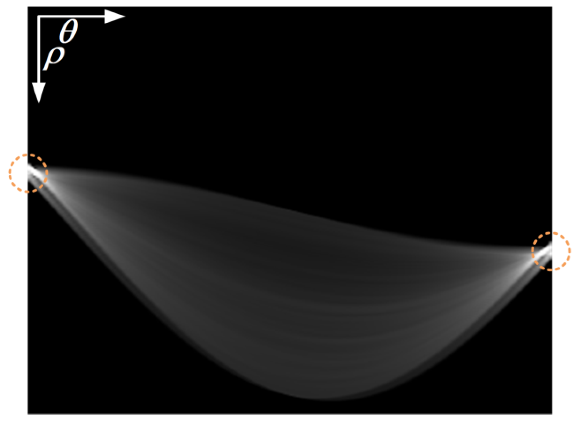
3.1. Image Domain Separation

First, it is assumed that the raw data have been subjected to range compression, and then HT is used to initially compensate the translation parameters, rough imaging is performed, and the ship target is reversed to the data domain. The HT was proposed by P. Hough in 1962. Its basic principle is to transform the curve in the image space into the parameter space and determine the description parameters of the curve by detecting the extreme points in the parameter space to realize the curve in the image extraction [47,48,49,50,51]. For slanted line detection, the expression of the HT in the standard parameterization method is

$$\rho =xcos\theta +ysin\theta \left(\rho \ge 0,0\le \theta \le \pi \right)$$

(14)

where $\rho$ and $\theta$ represent the vertical distance from the coordinate origin to the slanted line in the image space and the angle between the x-axis and the vertical line of the slanted line, respectively, as shown in Figure 3.

Equation (14) shows that the points on the slanted line become sinusoidal curves in the parameter space after undergoing HT. By performing HT on each point on the slanted line, the sinusoidal curves in the parameter space will intersect at the same point; as shown in Figure 3b, the horizontal and vertical coordinates of the point can be used to determine the slanted line in the image space.

It can be seen from Formula (4) that there is an error term in the phase term of sub-target $k$, and if no compensation is performed, the ISAR imaging quality will be reduced. When the sub-target $k$ moves in a slanted line with uniform acceleration, its translational component can be shown as

$$\Delta R\left(t_m\right)\cong \alpha +\beta t_m+\frac{\gamma }{2}{t}_m{}^2$$

(15)

where $\Delta R\left(t_m\right)$ represents the difference between the ideal distance and the actual distance from the ship’s target scatterers to the airborne platform. At this point, only two coefficients $\beta$ and $\gamma$ need to be estimated. Assuming that the multi-target contains $K$ sub-targets, the ISAR data after range compression can be regarded as composed of $K$ clusters of slanted lines with different slopes. Suppose the discrete form of $s_r\left(\widehat{t},t_m\right)$ is $s_0\left(n,m\right)$, then any slanted line with slope ω on $s_0\left(n,m\right)$ will have a slope $\omega$ equal to

$$\begin{array}{c}\Omega =-\frac{M}{N}\frac{1}{\omega }\end{array}$$

(16)

where $M$ and $N$ represent the number of sampling points in cross-range and range, respectively. Let the slope of the slanted line of the sub-target obtained via the HT be $\hat{\Omega }$, combined with Formula (16), the rough estimate of $\beta$ can be obtained as ${\beta }^{in}=-\frac{M}{N}\frac{1}{\hat{\Omega }}\frac{c}{2f_r}PRF$, where $f_r$ is the range sampling rate, and pulse repetition frequency is the $PRF$. According to ${\beta }^{in}$, the compensation function $\exp \left[j\frac{4\pi }{c}\left(f_c+f_r\right){\beta }^{in}{t}_m\right]$ can be constructed to complete the first-order phase of coarse compensation. In addition, before using the HT, the edge detection algorithm can be used to accurately locate the slanted line in the image, and the coherent speckle noise suppression process can be used for noise suppression, which can further improve the estimation accuracy of the slanted line slope.

After the rough estimation of the first-order phase error, the literature [52] is used to compensate for the remaining phase of the sub-target finely; the specific steps are as follows.

Step 1: Set the search range $\widehat{\beta }$ and step size of coefficient $\beta$ according to ${\beta }^{in}$; heuristically set the search range $\widehat{\gamma }$ and step size of coefficient $\gamma$.

Step 2: Compensate the phase by using the compensation function $\exp \left[j\frac{4\pi }{c}\left(f_c+f_r\right)\left({\beta }^{in}{t}_m+\frac{\widehat{\gamma }}{2}{t}_m{}^2\right)\right]$, and search the coefficient $\gamma$ linearly according to the principle of minimum entropy.

Step 3: When the entropy value is minimized, the value of the coefficient γ is obtained, and the compensation function $\exp \left[j\frac{4\pi }{c}\left(f_c+f_r\right)\left(\widehat{\beta }{t}_m+\frac{\gamma }{2}{t}_m{}^2\right)\right]$ is used to re-linearly search the coefficient according to the principle of the minimum image entropy $\beta$.

Step 4: Construct the phase item $\exp \left[j\frac{4\pi }{c}\left(f_c+f_r\right)\left(\beta t_m+\frac{\gamma }{2}{t}_m{}^2\right)\right]$ to complete the compensation.

Repeat the above process for the rest of the sub-targets to obtain the ISAR rough compensation images.

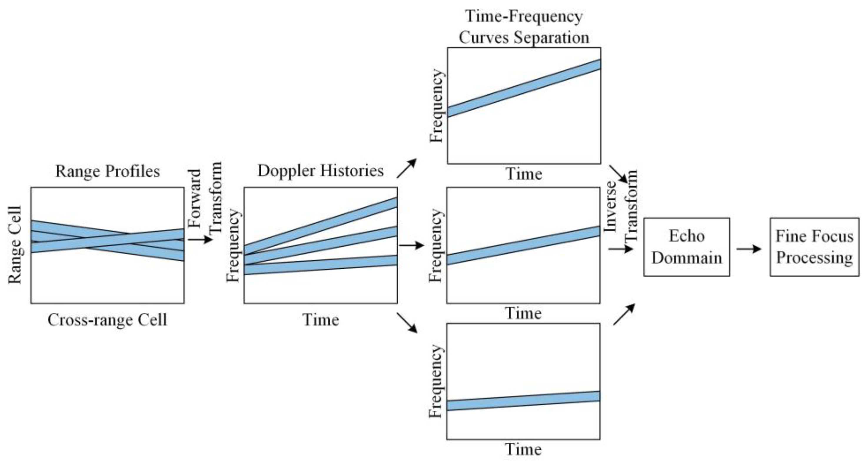
3.2. Signal Domain Separation

Through the above steps, the ISAR rough motion compensation images of all sub-targets can be obtained. However, when the sub-targets are close to each other, there is no way to accurately separate them in the image domain, and there are still echoes of the remaining sub-targets remaining in them, affecting the final imaging quality. Hence, further separation of the echoes in the time–frequency domain is considered to extract the complete target echo.

Signals can be observed from two different perspectives: the time domain and the frequency domain. Some signals that are not easy to process in the time domain are usually simpler in the frequency domain. The Fourier transform and its inverse transform describe the relationship between a time-domain signal $x\left(t\right)$ and its spectrum $X\left(f\right)$

$$X\left(f\right)={{\displaystyle \int }}_{-\infty }^{\infty }x\left(t\right)e^{-j2\pi ft}dt.$$

(17)

$$x\left(t\right)=\frac{1}{2\pi }{{\displaystyle \int }}_{-\infty }^{\infty }X\left(f\right)e^{j2\pi ft}df.$$

(18)

The Fourier transform is a global transform that decomposes the signal as a whole. However, in practical applications, most signals have non-stationary characteristics, and the Fourier transform cannot reflect the local characteristics of the signal well. If the change of the spectrum $X\left(f\right)$ with time $t$ can be obtained, the signal can be more intuitively understood. The joint time–frequency form $X\left(t,f\right)$ of the signal is used to meet this requirement. It is difficult to see the modulation type and related characteristics from the time-domain waveform or spectrum, but by converting the signal to the time–frequency plane, the linear relationship between the time and frequency of the signal can be clearly seen.

The classical method for time–frequency analysis is the STFT [53,54,55,56,57,58], which is implemented by performing the Fourier transform of the time-domain signal in segments, assuming the signal to be smooth within each segment, as a way of obtaining the signal’s local properties over that period of time. The specific expressions are as follows:

$$STF{T}_x\left(t,\omega \right)={{\displaystyle \int }}_{-\infty }^{\infty }x\left(\tau \right)h\left(\tau -t\right)\exp \left(-j\omega \tau \right)d\tau .$$

(19)

According to Formula (19), the difference between the STFT and the ordinary Fourier transform is the extra rectangular window function $h\left(t\right)$. When the width of the window function tends to infinity when $h\left(t\right)=1$, then the STFT is equivalent to the conventional Fourier transform. STFT analyzes signals within a finite window width each time, equivalent to performing a Fourier transform of the signal $x\left(t\right)$ at a certain moment, thus obtaining the local characteristics of the signal. The difficulty of STFT lies in the selection of the window width, which often fails to consider the frequency resolution and time resolution. However, for multi-target separation imaging, the frequency resolution requirement is not high, and what is more needed is to avoid cross-term interference as much as possible, so the time–frequency analysis using STFT is usually a better choice.

Time–frequency analysis was performed using STFT to separate the sub-targets by differences in Doppler histories.

Step 1: STFT is performed on the first range cell of the multi-target echo, and the time–frequency analysis curve corresponding to each sub-target is obtained in the time–frequency plane, and its slope and initial frequency are not the same.

Step 2: Separating different time–frequency curves in the time–frequency plane using masking techniques.

Step 3: The separated time–frequency curves are inversely STFT to the data domain separately to obtain the echo signal for each sub-target within that range cell.

Step 4: Repeat the above steps for all range cells containing target echoes, resulting in an overall echo for each sub-target.

The specific process is shown in Figure 4.

For multi-ship targets that are close to each other and have little difference in motion parameters, high-precision echo separation can be accomplished after the two key steps proposed in this paper, after which further fine focusing is performed on each target to obtain high-resolution ISAR images.

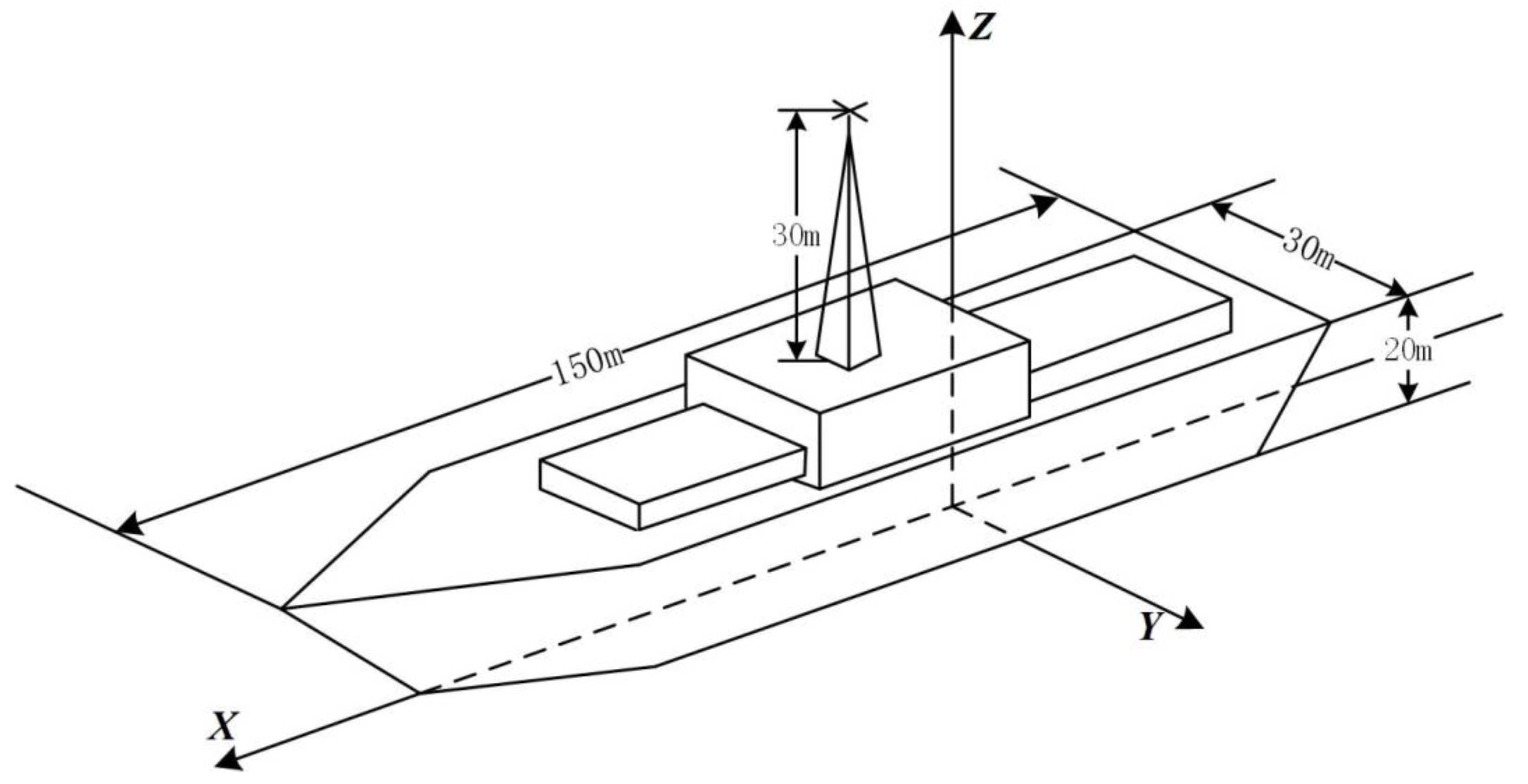
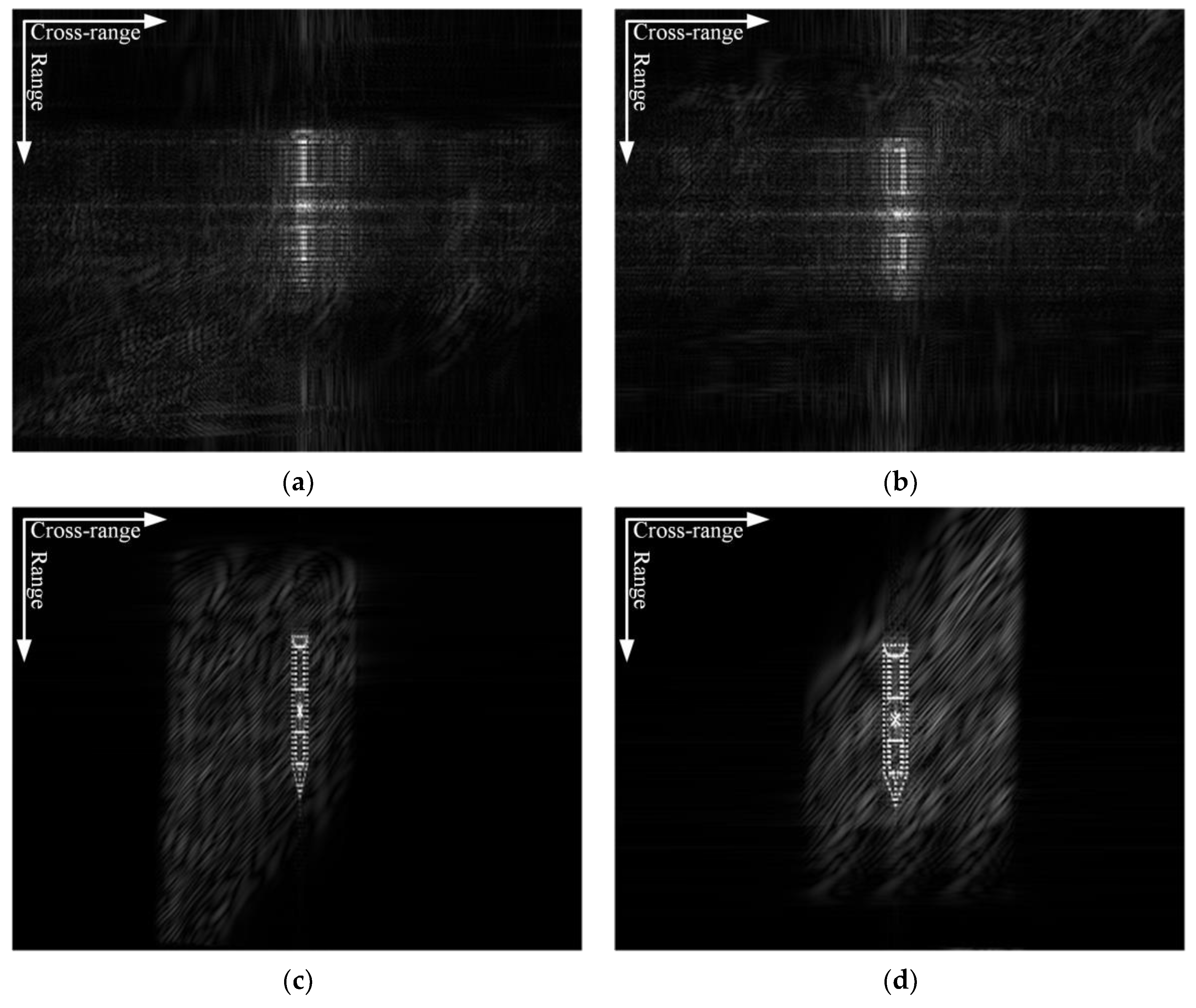
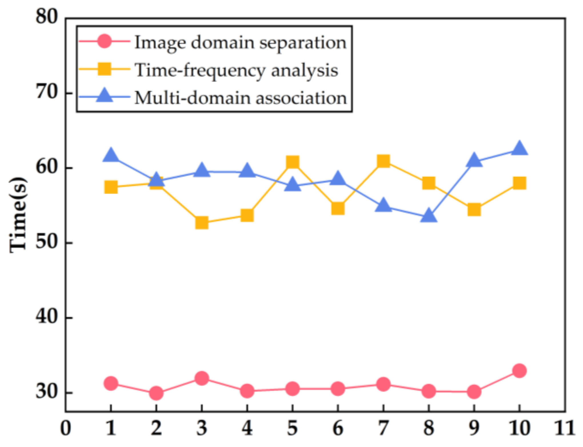
4. Experimental Results and Analysis

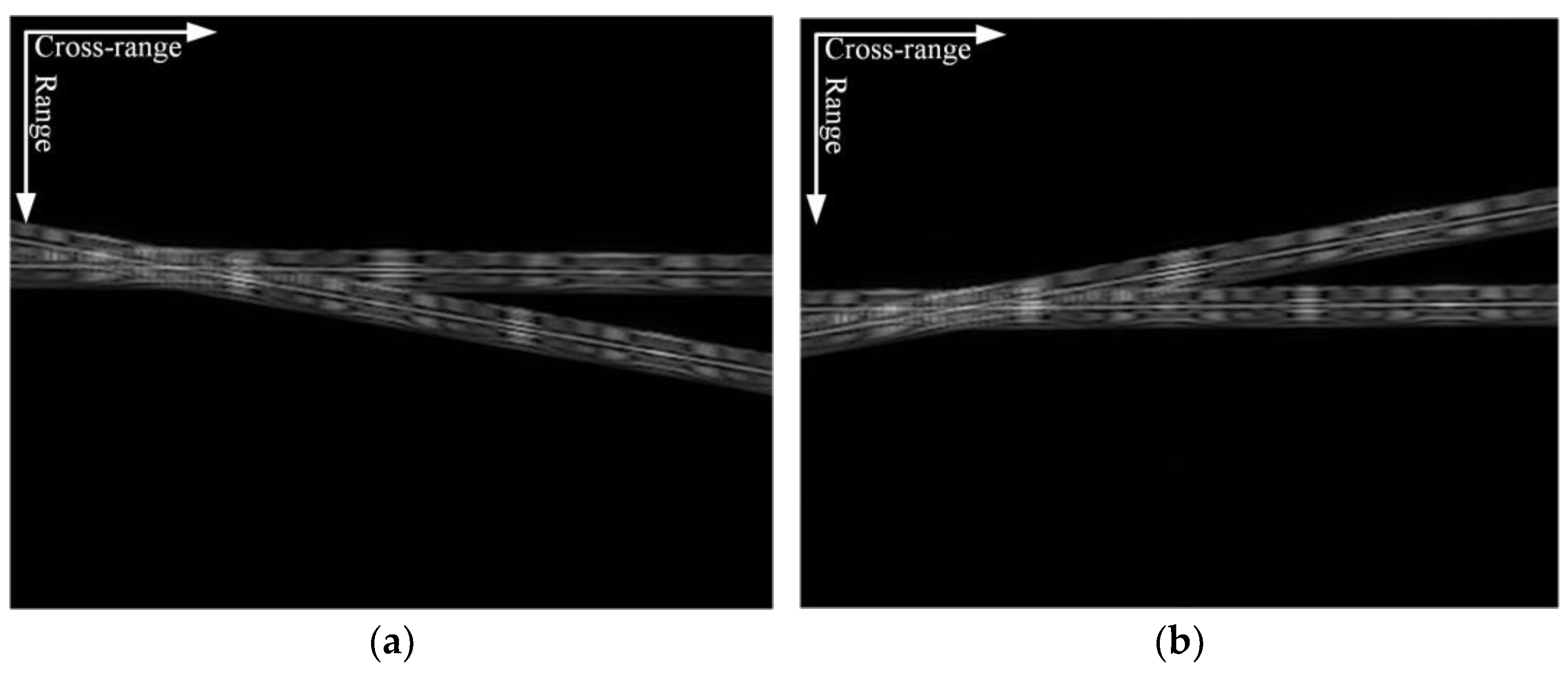
4.1. Simulated Data Processing Results

To verify the effectiveness of the proposed method, simulation experiments were first conducted. The ship model in the simulation experiment consists of 301 scatterers, and the ship model is shown in Figure 5.

The targets are assumed to have equal scattering magnitude and are in uniform linear motion on the sea surface; their simulation parameters are shown in

Table 1. Main radar parameters of a multi-target simulation experiment.

Radar Parameters	Value
Carrier frequency	10 GHz
Bandwidth	210 MHz
Pulse repetition frequency	400 Hz
Pulse width	10 $\mathsf{\mu }\mathrm{s}$
Airborne velocity	120 m/s
Ship1 velocity	18 Kn
Ship2 velocity	23 Kn
Radar height	2000 m
Straight-line distance betweenship targets	120 m

. The one-dimensional range profile is shown in Figure 6a. Figure 6a shows that the one-dimensional range profiles of two targets intersect, and they cannot be distinguished from the range or cross-range alone.

The results of doing time–frequency analysis and accumulating the range cell containing two targets using STFT are shown in Figure 6b, which shows that due to the closer motion parameters of the two ship targets, the Doppler history appears to be intersected, and it is not possible to separate them into images from the time–frequency domain alone. The HT-based multi-target imaging method is utilized to compensate for the uniform translational motion of the target, and the HT results are given in Figure 7, where two local peaks can be clearly seen.

The positions of peak 1 and peak 2 are detected, and thus, the slopes of the one-dimensional range profiles of the corresponding sub-targets are calculated. The minimum image entropy search coefficient is further utilized to complete the preliminary translational compensation, and the compensated one-dimensional range profile is shown in Figure 8a,b.

The rough imaging results are obtained by applying the cross-range Fourier transform to the data, as illustrated in Figure 9a,b. It can be shown that the sub-targets cannot be entirely intercepted from the image domain.

Next, the individual ship targets are inverted back to the data domain, and the time–frequency analysis is performed using STFT, as shown in Figure 10a,b. It can be found that the Doppler history of the two ship targets can be clearly separated in the time–frequency domain after the image domain separation.

The final imaging results are shown in Figure 11. Figure 11a,b show the imaging results based on the image-domain separation imaging method, Figure 11c,d show the imaging results based on the time–frequency analysis of the separation imaging method, and Figure 11e,f show the imaging results of the proposed method.

According to Figure 11, the proposed method produces superior imaging results than the classic image separation imaging method. Due to Doppler history aliasing being unable to be completely separated from the echo data, based on the time–frequency analysis of the sub-ship target, the separation imaging results are closer to the rough imaging results based on the image domain separation imaging. To evaluate the image quality, Shannon entropy is adopted here.

Table 2. Evaluation metrics for multi-target imaging results from simulated data.

Target	Method	IC	IE	IP
Sub-ship target 1	Based on image domain	2.9128	6.1450	3.3464 × 105
	Based on time–frequency analysis	6.5186	6.0113	3.5459 × 105
	Based on multi-domain association	7.9994	5.1444	1.1803 × 106
Sub-ship target 2	Based on image domain	2.8358	6.1988	1.2049 × 106
	Based on time–frequency analysis	5.9921	5.9540	1.2574 × 106
	Based on multi-domain association	7.1528	5.1597	1.6022 × 106

shows the Image Entropy (IE), Image Contrast (IC), and Image Peak (IP) of the imaging results, and it can be shown that the proposed method has the lowest IE and the highest IC, which further proves the superiority of the imaging quality of the proposed method.

4.2. Measured Data Processing Results

The measured data are airborne L-band SAR data, and the radar bandwidth is 200 MHz. In this paper, the original echo data are imaged, and the image of the target ship is intercepted. Finally, the ship image is inversely transformed to obtain the equivalent raw data of the ship target [59]. The scene in which the measured data are located contains more serious interference noise, as shown in Figure 12, which further demonstrates the performance of the proposed method in a low signal-to-noise ratio environment.

The HT and minimum entropy criteria were used for translational compensation, resulting in the one-dimensional range profile results shown in Figure 13a,b. The extracted echo data of the ship target using the method in this section are shown in Figure 13c,d.

The final imaging results are shown in Figure 14. Figure 14a,b show the imaging results based on the image-domain separation imaging method, Figure 14c,d show the imaging results based on the time–frequency analysis of the separation imaging method, and Figure 14e,f show the imaging results of the proposed method.

From Figure 14, it can be seen that the traditional image domain separation method cannot accurately focus on its own ship target due to the presence of echo interference from other targets. The traditional time–frequency analysis method cannot accurately extract the echo data of the two ship targets. The sub-target echoes of the method proposed in this paper can be completely extracted and can complete the subsequent fine-focusing processing, which proves that it still has good feasibility and effectiveness in the measured data. IE and IC are also used to evaluate the image quality. As shown in

Table 3. Evaluation metrics for multi-target imaging results from measured data.

Target	Method	IC	IE	IP
Sub-ship target 1	Based on image domain	2.1233	5.8923	2.8353 × 104
	Based on time–frequency analysis	3.6108	5.7162	1.1138 × 104
	Based on multi-domain association	11.4638	5.6643	3.1239 × 104
Sub-ship target 2	Based on image domain	2.3459	5.7641	1.6443 × 104
	Based on time–frequency analysis	4.6659	5.7390	1.8430 × 104
	Based on multi-domain association	10.6554	5.7152	1.9326 × 104

, the proposed method has the lowest image entropy with the highest image contrast, which further proves the superiority of the imaging quality of the proposed method.

5. Discussion

In this work, methods for separating and imaging multi-ship targets were investigated. By employing a multi-domain joint imaging approach, favorable imaging results were achieved. Firstly, coarse separation of ship targets was performed in the image domain. Then, fine separation of the echo data of ship targets was carried out in the signal domain. Finally, fine image processing of the sub-targets was performed, and the method’s effectiveness was validated using quantitative evaluation metrics.

To further validate the superiority of the proposed method, this paper also compares it with a multi-target separation imaging algorithm based on the Keystone transform [60]. The Keystone transform algorithm is widely used for motion compensation in ISAR [61,62] applications. Transforming a slow-time variable into a virtual slow-time variable enables arbitrary linear range migration correction without the need for prior information about the targets. The simulation data utilized in Section 4.1 were employed, and the experimental outcomes are presented in Figure 15. From the results, it can be observed that the multi-target separation algorithm based on the Keystone transform fails to extract the complete sub-target echo data, resulting in interference from echoes of other targets in the sub-target imaging results. This further validates the superiority of the proposed method in this paper. In addition, this paper also investigates the computational time of the classical image domain separation method, the time-frequency analysis method, and the proposed method. Through ten experiments, it is found that the classical image domain separation method has relatively low computational time, while the time–frequency analysis method and the proposed method have similar computational times. The results are shown in Figure 16. However, for research, it is worthwhile to use the method proposed in this paper to improve the imaging results.

Finally, through experiments, it is evident that although the method proposed in this paper can achieve satisfactory imaging results overall, it has a relatively long computational time. Therefore, in practical engineering applications, it may not meet real-time requirements. As a result, further improvements are necessary to enhance the algorithm’s efficiency.

6. Conclusions

This paper proposes a multi-target imaging method for separating the target echoes of a ship formation with high accuracy. Aiming at the similarity of position and motion between multi-ship targets, the echoes and Doppler history are all aliased after the range compression, and as the separation of imaging cannot be effectively carried out in a single domain, the HT and the STFT accomplish the separation of multi-target echoes in the joint image domain and the time–frequency domain. The effectiveness of the method is verified by the experimental results of a simulation and measured data. The proposed method separates the sub-target echoes more completely than the traditional echo separation method, and the resulting image has the highest image contrast with the lowest image entropy. However, it is worth noting that ships, as military targets, have high real-time ISAR imaging requirements. Compared with the traditional image domain separation method, the proposed method is more complex. However, experimental results show that it provides higher robustness in sub-target echo separation, which is worthwhile in practice. Therefore, to achieve an efficient and highly accurate multi-ship target imaging method in the future, research can be conducted in the following directions:

Algorithm optimization: Improve and optimize the existing multi-ship target imaging algorithms to reduce computational load and enhance processing speed. Techniques such as parallel computing can be employed to improve algorithm efficiency and computational capability.

Feature extraction and selection: Research effective methods for feature extraction and selection specifically for multi-ship target ISAR data. These methods aim to reduce data redundancy and highlight the features of sub-targets. By doing so, it is possible to reduce computational load while preserving imaging quality.

Real-time application and system integration: Apply the research findings to real-world scenarios, considering the requirements of real-time processing and system integration. Design efficient real-time imaging algorithms that can rapidly and accurately process ISAR data of multi-ship targets in practical engineering applications.

The research direction and methods described above can enable the development of an efficient and highly accurate multi-ship target imaging method, meeting the demands of practical engineering applications. This approach holds significant potential for widespread application in areas such as military operations, ocean monitoring, and shipping and can provide support for further advancements in these fields.

References

1. Cai, Y.H.; Li, J.F.; Yang, Q.Y.; Liang, D.; Liu, K.Y.; Zhang, H.; Lu, P.P.; Wang, R. First Demonstration of RFI Mitigation in the Phase Synchronization of LT-1 Bistatic SAR. IEEE Trans. Geosci. Remote Sens. 2023. ahead of print. [Google Scholar] [CrossRef]
2. Yang, S.; Li, S.; Fan, H.; Li, H. An Effective Translational Motion Compensation Approach for High-Resolution ISAR Imaging with Time-Varying Amplitude. IEEE Geosci. Remote Sens. Lett. 2023, 20, 4007805. [Google Scholar] [CrossRef]
3. Vehmas, R.; Neuberger, N. Inverse Synthetic Aperture Radar Imaging: A Historical Perspective and State-of-the-Art Survey. IEEE Access 2021, 9, 113917–113943. [Google Scholar]
4. Zhang, T.; Li, Y.; Wang, J.; Xing, M.; Guo, L.; Zhang, P. A modified range model and extended omega-k algorithm for high-speed-high-squint sar with curved trajectory. IEEE Trans. Geosci. Remote Sens. 2023, 61, 5204515. [Google Scholar] [CrossRef]
5. Ding, J.; Li, Y.; Wang, J.; Li, M.; Wei, J. Joint motion compensation and distortion correction for maneuvering target bistatic isar imaging based on parametric minimum entropy optimization. IEEE Trans. Geosci. Remote Sens. 2022, 60, 1–19. [Google Scholar]
6. Li, Y.; Wang, J.; Wang, Y.; Zhang, P.; Zuo, L. Random frequency coded waveform optimization and signal coherent accumulation against compound deception jamming. IEEE Trans. Aerosp. Electron. Syst. 2023, 59, 4434–4449. [Google Scholar] [CrossRef]
7. Zuo, L.; Hu, J.; Sun, H.; Gao, Y. Resource allocation for target tracking in multiple radar architectures over lossy networks. Signal Process. 2023, 208, 108973. [Google Scholar]
8. Wang, Y.; Zhou, X.Y.; Lu, X.F.; Li, Y.J. An approach of motion compensation and ISAR imaging for micro-motion targets. J. Syst. Eng. Electron. 2021, 32, 68–80. [Google Scholar]
9. Sun, S.B.; Liang, G.L. ISAR Imaging of Targets with Complex Motions Based on the Keystone Time-Chirp Rate Distribution. Int. J. Remote Sens. 2018, 39, 1770–1781. [Google Scholar] [CrossRef]
10. Chen, C.C.; Andrews, H.C. Target-motion induced radar imaging. IEEE Trans. Aerosp. Electron. Syst. 1980, 16, 2–14. [Google Scholar] [CrossRef]
11. Wang, J.; Zhang, L.; Du, L.; Yang, D.; Chen, B. Noise-Robust Motion Compensation for Aerial Maneuvering Target ISAR Imaging by Parametric Minimum Entropy Optimization. IEEE Trans. Geosci. Remote Sens. 2019, 57, 4202–4217. [Google Scholar]
12. Wahl, D.E.; Eichel, P.H.; Ghiglia, D.C.; Jakowatz, C.V. Phase gradient autofocus–A robust tool for high resolution SAR phase correction. IEEE Trans. Aerosp. Electron. Syst. 1994, 30, 827–835. [Google Scholar] [CrossRef]
13. Itoh, T.; Sueda, H.; Watanabe, Y. Motion compensation for ISAR via centroid tracking. IEEE Trans. Aerosp. Electron. Syst. 1996, 32, 1191–1197. [Google Scholar] [CrossRef]
14. Shao, S.; Zhang, L.; Liu, H. High-Resolution ISAR Imaging and Motion Compensation with 2-D Joint Sparse Reconstruction. IEEE Trans. Geosci. Remote Sens. 2020, 58, 6791–6811. [Google Scholar] [CrossRef]
15. Gao, Y.; Xing, M.; Li, Y.; Sun, W.; Zhang, Z. Joint Translational Motion Compensation Method for ISAR Imagery Under Low SNR Condition Using Dynamic Image Sharpness Metric Optimization. IEEE Trans. Geosci. Remote Sens. 2022, 60, 5108515. [Google Scholar]
16. Chen, J.; Liang, B.; Yang, D.-G.; Zhao, D.-J.; Xing, M.; Sun, G.-C. Two-Step Accuracy Improvement of Motion Compensation for Airborne SAR With Ultrahigh Resolution and Wide Swath. IEEE Trans. Geosci. Remote Sens. 2019, 57, 7148–7160. [Google Scholar]
17. Wang, Y.; Chen, J.W.; Liu, Z.; Liu, A.F. Research on ISAR Imaging of Multiple Moving Targets. J. Astronaut. 2005, 26, 450–454. [Google Scholar]
18. Li, Y.N.; Fu, Y.W.; Li, X. The Summarization of Multiple Target ISAR Imaging. Signal Process. 2009, 25, 1092–1096. [Google Scholar]
19. Li, Y.; Wang, J.; Liu, R.; Ding, J.; Zhang, P.; Xing, M. Joint Translational Motion Compensation for Multi-target ISAR Imaging Based on Integrated Kalman Filter. IEEE Trans. Geosci. Remote Sens. 2023, 61, 5108716. [Google Scholar]
20. Bao, Z.; Sun, C.Y.; Xing, M.D. Time-frequency approaches to ISAR imaging of maneuvering targets and their limitations. IEEE Trans. Aerosp. Electron. Syst. 2001, 37, 1091–1099. [Google Scholar]
21. Berizzi, F.; Mese, E.D.; Diani, M.; Martorella, M. High-resolution ISAR imaging of maneuvering targets by means of the range instantaneous Doppler technique: Modeling and performance analysis. IEEE Trans. Image Process. 2001, 10, 1880–1890. [Google Scholar] [CrossRef]
22. ZZhu, D.; Yin, J.; Wu, X.Q.; Zhou, J.J. ISAR Imaging of Multiple Moving Targets Using Time-Frequency Representations. Mod. Radar 1993, 15, 33–37. [Google Scholar]
23. Wu, J.W. ISAR Imaging of Multi-Target; Harbin Institute of Technology: Harbin, China, 2012. [Google Scholar]
24. Chen, V.C.; Qian, S. Joint time-frequency transform for radar range-Doppler imaging. IEEE Trans. Aerosp. Electron. Syst. 1998, 34, 486–499. [Google Scholar]
25. Chen, J.; Xiao, H.T.; Song, Z.Y.; Fan, H.Q. Simultaneous ISAR imaging of group targets flying in formation. Chin. J. Aeronaut. 2014, 27, 1554–1561. [Google Scholar] [CrossRef]
26. Yang, J.; Wang, M.S.; Bao, Z. A Real-time Implementation Technique of Multi-target ISAR Imaging. Acta Electron. Sin. 1995, 23, 60. [Google Scholar]
27. Chen, W.C.; Xing, M.D. An ISAR Imaging Algorithm for Multiple Targets Based on Keystone Transformation. Mod. Radar 2005, 27, 40–42. [Google Scholar]
28. Park, S.H.; Park, K.K.; Jung, J.H.; Kim, H.T.; Kim, K.T. ISAR Imaging of Multiple Targets Using Edge Detection and Hough Transform. J. Electromagn. Waves Appl. 2008, 22, 365–373. [Google Scholar]
29. Park, S.H.; Kim, H.T.; Kim, K.T. Segmentation of ISAR Images of Targets Moving in Formation. IEEE Trans. Geosci. Remote Sens. 2010, 48, 2099–2108. [Google Scholar] [CrossRef]
30. Bai, X.R.; Zhou, F.; Xing, M.D.; Bao, Z. A Novel Method for Imaging of Group Targets Moving in a Formation. IEEE Trans. Aerosp. Electron. Syst. 2012, 50, 221–231. [Google Scholar]
31. Wu, X.Q.; Zhu, Z.D. Simultaneous imaging of multiple targets in an inverse synthetic aperture radar. In Proceedings of the IEEE Conference on Aerospace and Electronics, Dayton, OH, USA, 21–25 May 1990; pp. 210–214. [Google Scholar]
32. Zhu, Z.D.; She, Z.S.; Zhou, J.J. Multiple moving target resolution and imaging based on ISAR principle. In Proceedings of the IEEE 1995 National Aerospace and Electronics Conference, NAECON 1995, Dayton, OH, USA, 22–26 May 1995; pp. 982–987. [Google Scholar]
33. Chen, V.C.; Lu, Z.Z. Radar imaging of multiple moving targets. In Radar Processing Technology and Applications II; SPIE: Bellingham, WA, USA, 1997; Volume 3161, pp. 102–112. [Google Scholar]
34. Chen, V.C. Radar detection of multiple moving targets in clutter using time-frequency radon transform. In Signal and Data Processing of Small Targets 2002; SPIE: Bellingham, WA, USA, 2002; Volume 4728, pp. 48–59. [Google Scholar]
35. Chen, W.C. An Implementation Method of ISAR Imaging for Multiple Targets in Formation. Acta Electron. Sin. 2006, 34, 1119–1122. [Google Scholar]
36. Chen, J.; Xiao, H.T.; Fan, H.Q.; Song, Z.Y. ISAR Imaging of Multiple Moving Targets Using Signals Separation. In Proceedings of the 2013 International Conference on Mechatronic Sciences, Electric Engineering and Computer (MEC), Shenyang, China, 20–22 December 2013; pp. 1156–1159. [Google Scholar]
37. Dong, X.; Zhang, Y.H.; Gu, X.; Zhai, W.S. ISAR imaging of multiple targets based on sparse representations. In Proceedings of the 2015 IEEE International Conference on Microwaves, Communications, Antennas and Electronic Systems (COMCAS), Tel Aviv, Israel, 2–4 November 2015; pp. 1–4. [Google Scholar]
38. Zhang, D.; Feng, C.Q.; He, S.S.; Luo, Y.Z.; Luo, X. Multi Targets Echo Signal Separation Algorithm Based on Joint Time-frequency Filtering. Fire Control Command Control 2015, 40, 12–15. [Google Scholar]
39. Zhou, F.; Bai, X.; Xing, M.; Bao, Z. Analysis of wide-angle radar imaging. IET Radar Sonar Navig. 2011, 5, 449–457. [Google Scholar] [CrossRef]
40. Liu, L.; Zhou, F.; Tao, M.; Zhang, Z. A Novel Method for Multi-Targets ISAR Imaging Based on Particle Swarm Optimization and Modified CLEAN Technique. IEEE Sens. J. 2016, 16, 97–108. [Google Scholar] [CrossRef]
41. Huang, X.; Tang, S.; Zhang, L.; Li, S. Ground-Based Radar Detection for High-Speed Maneuvering Target via Fast Discrete Chirp-Fourier Transform. IEEE Access 2019, 7, 12097–12113. [Google Scholar] [CrossRef]
42. Mallat, S.G.; Zhang, Z.F. Matching pursuits with time-frequency dictionaries. IEEE Trans. Signal Process. 1993, 41, 3397–3415. [Google Scholar] [CrossRef]
43. Ryu, B.-H.; Lee, I.-H.; Kang, B.-S.; Kim, K.-T. Frame Selection Method for ISAR Imaging of 3-D Rotating Target Based on Time–Frequency Analysis and Radon Transform. IEEE Sens. J. 2022, 22, 19953–19964. [Google Scholar] [CrossRef]
44. Jeong, S.-J.; Kang, B.-S.; Kang, M.-S.; Kim, K.-T. ISAR Cross-Range Scaling Using Radon Transform and its Projection. IEEE Trans. Aerosp. Electron. Syst. 2018, 54, 2590–2600. [Google Scholar] [CrossRef]
45. Kong, L.; Zhang, W.; Zhang, S.; Zhou, B. Radon transform and the modified envelope correlation method for ISAR imaging of multi-target. In Proceedings of the 2010 IEEE Radar Conference, Arlington, VA, USA, 10–14 May 2010; pp. 637–641. [Google Scholar]
46. Hongyin, S.; Yue, L.; Jianwen, G.; Mingxin, L. ISAR autofocus imaging algorithm for maneuvering targets based on deep learning and keystone transform. J. Syst. Eng. Electron. 2020, 31, 1178–1185. [Google Scholar] [CrossRef]
47. Carlson, B.D.; Evans, E.D.; Wilson, S.L. Search radar detection and track with the Hough transform. IEEE Trans. Aerosp. Electron. Syst. 1994, 30, 102–108. [Google Scholar] [CrossRef]
48. Liang, Y.; Bai, P.; Zhang, Q.; Zhu, X.P.; Wang, M. Analysis and extraction of micro-doppler features in FMCW-ISAR using a Modified Extended Hough Transform. In Proceedings of the 2011 IEEE CIE International Conference on Radar, Chengdu, China, 24–27 October 2011; pp. 1652–1655. [Google Scholar]
49. Fei, L.; Bo, J.; Hong-Wei, L.; Bo, F. Cross-range scaling of interferometric ISAR based on Randomized Hough Transform. In Proceedings of the 2011 IEEE International Conference on Signal Processing, Communications and Computing (ICSPCC), Xi’an, China, 25–27 October 2011; pp. 1–4. [Google Scholar]
50. Fu, X.J.; Guo, M.G. ISAR imaging for multiple targets based on randomized Hough transform. In Proceedings of the 2008 Congress on Image and Signal Processing, Sanya, China, 27–30 May 2008; pp. 238–241. [Google Scholar]
51. Zhang, Y.A.; Zhang, D.C.; Chen, W.D.; Wang, D.J. ISAR imaging of multiple moving targets based on RSPWVD-Hough transform. In Proceedings of the 2008 Asia-Pacific Microwave Conference, Hong Kong, China, 16–20 December 2008; pp. 1–4. [Google Scholar]
52. Martorella, M.; Berizzi, F.; Haywood, B. Contrast Maximisation based technique for 2-D ISAR autofocusing. IEE Proc. Radar Sonar Navig. 2005, 152, 253–262. [Google Scholar] [CrossRef]
53. Cohen, L. Time-frequency distributions—A review. Proc. IEEE 1989, 77, 941–981. [Google Scholar]
54. Khan, T.A.; Zulfiqar, S.; Irfan, M. An Efficient ISAR Image Enrichment and Feature Abstraction of Moving Targets using Time-Frequency Transforms. In Proceedings of the 2023 International Conference on Business Analytics for Technology and Security (ICBATS), Dubai, United Arab Emirates, 7–8 March 2023; pp. 1–5. [Google Scholar]
55. Sejdić, E.; Djurović, I.; Jiang, J. Time-frequency feature representation using energy concentration: An overview of recent advances. Digit. Signal Process. 2009, 19, 153–183. [Google Scholar]
56. Yang, Y.; Cheng, Y.; Wu, H.; Yang, Z.; Wang, H. Time–Frequency Feature Enhancement of Moving Target Based on Adaptive Short-Time Sparse Representation. IEEE Geosci. Remote Sens. Lett. 2022, 19, 4026205. [Google Scholar]
57. Pei, S.C.; Huang, S.G. STFT with Adaptive Window Width Based on the Chirp Rate. IEEE Trans. Signal Process. 2012, 60, 4065–4080. [Google Scholar] [CrossRef]
58. Zhong, J.G.; Huang, Y. Time-Frequency Representation Based on an Adaptive Short-Time Fourier Transform. IEEE Trans. Signal Process. 2010, 58, 5118–5128. [Google Scholar]
59. Martorella, M.; Berizzi, F.; Giusti, E.; Bacci, A. Refocussing of moving targets in SAR images based on inversion mapping and ISAR processing. In Proceedings of the 2011 IEEE RadarCon (RADAR), Kansas City, MO, USA, 23–27 May 2011; pp. 68–72. [Google Scholar]
60. Zhao, J.; Zhang, Y.Q.; Wang, X.; Wang, S.; Shang, F. A Novel Method for ISAR Imaging of Multiple Maneuvering Targets. Prog. Electromagn. Res. M 2019, 81, 43–54. [Google Scholar] [CrossRef]
61. Xing, M.D.; Wu, R.B.; Lan, J.Q.; Bao, Z. Migration through resolution cell compensation in ISAR imaging. IEEE Geosci. Remote Sens. Lett. 2004, 1, 141–144. [Google Scholar] [CrossRef]
62. Lv, X.L.; Xing, M.D.; Zhang, S.H.; Bao, Z. Keystone transformation of the Wigner-Ville distribution for analysis of multicomponent LFM signals. Signal Process. 2009, 89, 791–806. [Google Scholar] [CrossRef]
Figure 1. Multi-ship target geometry model.
Remotesensing 15 04878 g001
Figure 2. Flowchart of the proposed algorithm.
Remotesensing 15 04878 g002
Figure 3. Schematic diagram of the Hough transform. (a) Image-space results. (b) Parameter-space results.
Remotesensing 15 04878 g003
Figure 4. Imaging flowchart based on time–frequency analysis.
Remotesensing 15 04878 g004
Figure 5. Three-dimensional view of the ship model.
Remotesensing 15 04878 g005
Figure 6. One-dimensional range profile and time–frequency distribution of a multi-ship target. (a) One-dimensional range profile of a multi-ship target. (b) Time–frequency distribution of multi-ship targets.
Remotesensing 15 04878 g006
Figure 7. ISAR echo Hough transform results for two targets.
Remotesensing 15 04878 g007
Figure 8. Multi-target translational compensation results. (a) Sub-ship target 1 rough compensation results. (b) Sub-ship target 2 rough compensation results.
Remotesensing 15 04878 g008
Figure 9. Multi-target rough imaging results. (a) Sub-ship target 1 rough imaging results. (b) Sub-ship target 2 rough imaging results.
Remotesensing 15 04878 g009
Figure 10. Multi-target time–frequency distribution. (a) Time–frequency distribution of sub-ship target 1. (b) Time–frequency distribution of sub-ship target 2.
Remotesensing 15 04878 g010
Figure 11. Simulation data multi-ship target imaging results (a) Image domain-based sub-ship target 1 separation imaging results. (b) Separation imaging results based on image domain sub-ship target 2. (c) Separation imaging results based on time–frequency analysis of sub-ship target 1. (d) Separation imaging results based on time–frequency analysis of sub-ship target 2. (e) Separation imaging results of sub-ship target 1 of the method proposed in this paper. (f) Separation imaging results of sub-ship target 2 of the method proposed in this paper.
Remotesensing 15 04878 g011aRemotesensing 15 04878 g011b
Figure 12. Measured data rage compressed echo.
Remotesensing 15 04878 g012
Figure 13. Measured data multi-ship target imaging results. (a) Sub-target 1 translation compensation results. (b) Sub-target 2 translation compensation results. (c) Extracted sub-target 1 echo. (d) Extracted sub-target 2 echo.
Remotesensing 15 04878 g013
Figure 14. Measured data multi-ship target imaging results. (a) Image domain-based sub-ship target 1 separation imaging results. (b) Separation imaging results based on image domain sub-ship target 2. (c) Separation imaging results based on time–frequency analysis of sub-ship target 1. (d) Separation imaging results based on time–frequency analysis of sub-ship target 2. (e) Separation imaging results of sub-ship target 1 of the method proposed in this paper. (f) Separation imaging results of sub-ship target 2 of the method proposed in this paper.
Remotesensing 15 04878 g014
Figure 15. Separation imaging results based on Keystone transform. (a) Sub-ship target 1 imaging results. (b) Sub-ship target 2 imaging results.
Remotesensing 15 04878 g015
Figure 16. Time consumption of image domain separation, time–frequency analysis, and multi-domain association.
Remotesensing 15 04878 g016