Abstract
In a space-based infrared system, the enhancement of targets plays a crucial role in improving target detection capabilities. However, the existing methods of target enhancement face challenges when dealing with multi-target scenarios and a low signal-to-noise ratio (SNR). Furthermore, false enhancement poses a serious problem that affects the overall performance. To address these issues, a new enhancement method for a dim moving multi-target with strong robustness for false enhancement is proposed in this paper. Firstly, multi-target localization is applied by spatial–temporal filtering and connected component detection. Then, the motion vectors of each target are obtained using optical flow detection. Finally, the consecutive images are convoluted in 3D based on the convolution kernel guided by the motion vectors of the target. This process allows for the accumulation of the target energy. The experimental results demonstrate that this algorithm can adaptively enhance a multi-target and notably improve the SNR under low SNR conditions. Moreover, it exhibits outstanding performance compared to other algorithms and possesses strong robustness against false enhancement.
1. Introduction
With the increase in human space activities, the application of space-based infrared target search and tracking technology in the military and civilian fields has become more and more extensive. Its main task is to analyze and identify targets, requiring detection of all targets in the image. However, there are some factors that limit the ability to detect, such as the dim and small features of the space targets caused by long detection distances, the deficiency of the detection system and the interference of the environment. In addition, when multiple targets appear in the field of view simultaneously, it is difficult to detect them all due to their unknown number and different states. Therefore, the enhancement of the dim moving target and improvement in its adaptability to multi-target has been regarded as the key to solve the above problems, as it can improve the SNR (signal-to-noise ratio) of the image and further improve the detection capability of space-based infrared target detection technology.
The existing infrared target enhancement methods can be divided into two categories: indirect target enhancement and direct target enhancement. Indirect enhancement that processes the background mainly relies on the background characteristics and can be divided into two types: spatial domain processing and transform domain processing. Background suppression methods in the spatial domain include histogram equalization [1], grayscale linear transformation, 2D least mean square filtering [2], max-mean filtering [3] and max-median filtering [4], Butterworth high-pass filtering, morphological filtering [5,6,7,8,9] and so on. In addition, the background suppression methods in the transform domain include the traditional frequency domain filtering [10] such as the ideal high-pass filter, Butterworth high-pass filtering and Gauss high-pass filtering, as well as the wavelet transform and its extended transform [11,12], such as the ridgelet transform, curvelet transform, contourlet transform and so on. These methods have the advantages of low computation and easy engineering implementation, and they can adapt to the multi-target situation because only the background characteristic has been considered. However, the performance of these methods is limited such that it cannot adapt to low SNR conditions. Meanwhile, a significant amount of noise remains after processing.
The methods of direct target enhancement are mainly based on the characteristics of the target, including the single-frame method based on the intensity attributes, the gradient attributes and the Gauss-like shape of the target, as well as the multi-frame method based on the motion characteristics of the target. Methods based on the intensity and gradient attributes of the target, such as the algorithms based on rough set theory [13,14], have limited applications for images with a low SNR. Methods based on the Gauss-like shape of the target, such as human visual characteristics (HVS)-based algorithms [15,16,17,18], do not take the interference of the background into account. Although the single-frame methods can adapt to multi-target conditions, they are prone to target misidentification and removal due to the limited available information. This makes it difficult to recover the targets in the subsequent processing. The multi-frame methods mainly based on the motion characteristics of the target perform better than the above algorithms because they utilize both the spatial and temporal characteristics of the targets. In particular, the model-based method [19,20] requires prior information about the target motion and therefore cannot enhance multiple targets because of inconsistency in the motion state of each target. Then, the algorithms based on a 3D matching filter [21], including the three-dimensional double-directional filtering (3DDDF) algorithm [22], 3D wide-to-exact search directional filtering [23] and three-dimensional collaborative filtering and spatial inversion (3DCFSI) algorithms [24], judge the existence of the target by traversing the trajectory and then enhance the target. In addition, the algorithms based on dynamic programming (DPA) [25,26,27,28,29,30] can enhance the target by optimizing the merit function. Unfortunately, when applied to multi-target scenarios, these approaches can be seriously affected by the blind pixels and noise. A blind pixel is easily identified as a target due to its high grayscale value. Once the blind pixel or noise is mistaken as the target during the judgment process, the performance of the algorithm will be greatly reduced, and the subsequent processing will be seriously affected.
Thus, the issues and challenges of the enhancement methods can be summed up into three points: stability at a low SNR, adaptability to multiple targets and robustness for false enhancement. In conclusion, a new enhancement method for a dim moving multi-target with strong robustness for false enhancement is proposed in this paper in order to meet the aforementioned requirements. Firstly, two filtering operations are conducted within a single frame using spatial information, and part of the noise is removed with temporal information. And the blind pixels are suppressed as well. After that, multiple targets are windowed through coarse positioning, and the optical flow of each target is detected within the corresponding window. Finally, the consecutive frames are locally convolved in 3D based on the individual optical flow. The experimental results demonstrate a significant improvement in the SNR, as well as the achievement of adaptive enhancement of multiple targets through the algorithm. Meanwhile, this method has strong robustness against false judgment, and it is not easy to cause false enhancement. Moreover, its performance surpasses that of other contrast algorithms.
The rest of this paper is structured as follows. In Section 2, the characteristics of infrared images with the dim moving multi-target are analyzed. Section 3 explains the proposed algorithm in detail. In Section 4, the experimental results and comparison are presented. Finally, a conclusion is given in Section 5.
2. Analysis of Dim Moving Infrared Target Images
Basically, there are three parts in a space-based infrared image: the targets, the background and the noise [31], which can be expressed as
where is the frame index; is the pixel’s coordinates; denotes the gray value at in frame k; and , and denote the target, background and noise gray values, respectively.
2.1. Characteristics of the Target
In theory, a space target can be viewed as a point light source [32,33] and the response of an imaging system to a point source can be described by the point spread function (PSF). Due to the influence and limitation of various factors, the actual optical system image of the point target is speckled, and then the PSF can be expressed by the Gauss function [34]:
Generally, the main intensity of a space target is concentrated in a pixel area of , and the intensity distribution will change with the change in its position, which can be expressed by the energy concentration [35]. Then, the energy concentration for the target of size is expressed as
In addition, the target center may be at the center of the pixel or across the pixel in the case of the same intensity. Figure 1 shows the shape of the target at the center of the pixel and across the pixel with different energy concentrations:
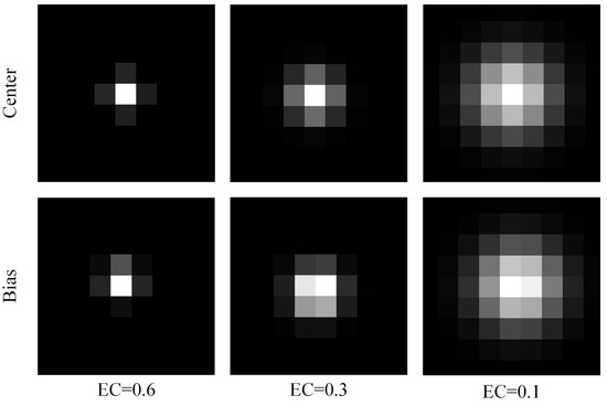
Figure 1.
Different forms of the target.
In addition to considering the radiation and geometric characteristics of space targets, the motion characteristics of targets can be analyzed based on the two aspects of the moving trajectory and moving velocity. The moving trajectory of the space target is determined by the height of the target, the detection distance, the detection angle and the resolution of the detector. The actual detection angle typically falls within the range of 0 to 90 degrees. Taking STSS satellite parameters as an example, the target’s trajectory appears as a nearly straight line when observed for a short duration (where the target moves approximately 200 pixels on the focal plane). The moving velocity of the target can be expressed using the ratio of angular acceleration to angular velocity. The angular velocity and acceleration of the target can be inferred from the orbit height, the height of the target, the detection distance and the detection angle. Analyzing the results reveals that the angular velocity is much larger than the angular acceleration. Thus, the space target moves at a relatively constant speed on the image plane under short-time observation [36].
In the actual scenario, multiple targets may appear simultaneously within the field of view, each with its own characteristics. The long-wave infrared image depicting 10 different simulated targets is shown in Figure 2.
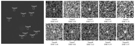
Figure 2.
The long-wave infrared image with 10 different simulated targets.
2.2. Characteristics of the Background and Noise
This paper primarily focuses on the space background without complex features and clouds in it. When observed by the infrared detection system outside the atmosphere, the background radiation mainly comes from the microwave emission from space matter.
The noise of the infrared detection system includes shot noise, 1/f noise, thermal noise and compound noise. In this paper, the total noise of the detector under the combined effect of various noises is analyzed. The noise distribution approximately follows a Gaussian distribution [37], and each pixel is independent in each frame.
In addition, infrared images often exhibit the presence of blind pixels, which greatly impact image quality. Blind pixels are abnormal pixels caused by infrared sensor degradation, which can be categorized as either fixed blind pixels or random blind pixels. Fixed blind pixels typically arise from process and material defects that cause irreversible damage to the pixel. The blind pixels manifest as overheated or over-darkened pixels, constituting a form of fixed noise in the detector. Specifically, superheated pixels appear as isolated bright spots in the image, affecting target identification.
In conclusion, target enhancement aims to suppress background, noise and blind pixels while simultaneously enhancing the energy of the targets, which is indeed a challenging task.
3. Method
To solve the problems discussed in Section 1, a new enhancement method for a dim moving multi-target with strong robustness for false enhancement is presented, considering the model of infrared images in Section 2. This algorithm consists of three parts: multi-target localization, motion detection by optical flow and 3D convolution. The flow chart of the proposed algorithm is shown in Figure 3.
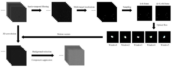
Figure 3.
The flow chart of the proposed algorithm.
3.1. Multi-Target Localization
According to the analysis in Section 2, the number of targets is uncharted, and every target has a different state of motion in the infrared images. As a result, multi-target localization forms the basis of the identification and separate processing of the target.
3.1.1. Spatio-Temporal Filtering and Blind Pixels Suppression
Considering the weakness and dispersion of the targets’ energy and the influence of the blind pixels and the noise, the infrared images are preprocessed.
Firstly, the energy of the targets is collected by spatial filtering, which can be expressed as
where is the region of size centered at and is the region of size , and . And denotes the gray value at on a frame of input images . Then, the blind pixels are suppressed by removing the isolated and bright spots:
where denotes the gray value at the center of , denotes the energy concentration while the blind pixels have a high value of it. And , considering that the practical energy concentration of the targets is less than 0.6. Then, the maximum filter is used to enlarge the targets:
where is the region of size centered at . At the same time, a new image sequence is generated.
In addition, there is a lot of random noise in infrared images, leading to the low SNR. Then, the temporal mean filter is used to partly remove the noise [38]. Meanwhile, the target will leave a track in the image due to its movement:
where is the frame index. is the number of accumulated frames.
3.1.2. Multi-Target Judgement and Rough Localization
The thick stripes of the target trajectories will appear obviously after the preprocessing. Based on it, the thresholding segmentation and the connected component detection are applied to confirm the number and the approximate moving area of the targets.
The image is usually segmented by the threshold before detection to remove most of the disruptive pixels:
where is the gray value, and the threshold , while and represent the mean and standard deviation of the image, respectively, and , which is a constant. Then, the first step of the connected component detection is 8-neighbor connected component labeling. After that, we obtain the connected components , and the thick stripes of the target trajectories can be extracted from among them. Considering both the size and the intensity of , the confidence is defined as
where denotes the number of non-zero pixels and denotes the gray values in . The confidence is used to judge whether the connected component is the thick stripe of the target trajectory that the weights of the connected components formed by the target will be greater than those formed by the noise or clutter:
where is the key threshold such that . We choose the connected components whose weights are times higher than the average value of all the connected components as the potential target region. Finally, the thick stripes of the target trajectories and the corresponding windows are obtained, while is the approximate moving area of the target during this time period. At the same time, a new image sequence is generated. The process is visualized in Figure 4.
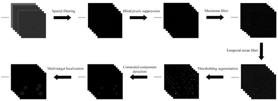
Figure 4.
The process of multi-target judgement and rough localization.
3.2. Motion Detection by Optical Flow
After multi-target rough localization, the motion vectors of each target can be obtained by using optical flow detection in the corresponding window.
3.2.1. Pyramid Lucas–Kanade (L-K) Optical Flow
Optical flow refers to the vector that represents the movement of moving objects or moving cameras between two consecutive images. It provides information about the instantaneous speed and direction of pixels in the imaging plane. The Lucas–Kanade (L-K) optical flow algorithm [39] is a classic algorithm used for estimating the sparse flow from a two-frame sequence. Furthermore, image pyramids are often used to improve the L-K optical flow algorithm.
The overall processing of the pyramid L-K optical flow algorithm is as follows:
- (1)
- The optical flow on the top layer of the image is calculated after the pyramid is built.
- (2)
- The displacement of the pixel on the current layer () is estimated initially by the calculation results of the optical flow on the upper layer (). Then, the optical flow on the current layer is calculated, which would be passed to the next layer ().
- (3)
- It is iterated until layer () is obtained. The resulting optical flow is the sum of all the layers.
3.2.2. Motion Detection by Pyramid L-K Optical Flow
Based on Section 3.1, only the thick stripes of the target trajectories are preserved in the processed image. And the displacement of these thick stripes in the adjacent frames can be equivalent to the motion of the target in the adjacent frames. As a result, the motion vector of the target can be obtained by detecting the optical flow of the thick stripe in the adjacent frames in the corresponding window.
In addition, there are two requirements for the optical flow method: brightness constancy and spatial coherence. On the one hand, the processed image is a binary image, and the pixel values of the thick stripes are all 1, so the first condition is satisfied. On the other hand, the thick stripes of the same target are almost the same shape in the adjacent frames, so the second condition is also satisfied.
Considering that the displacement of the target in the adjacent frames is very small, leading to the difficulty in detecting the optical flow, we use interlaced frames for the processing, which is called sampling:
where denotes the pyramid L-K optical flow algorithm, is the target window and is the image processed by algorithm and is the number of frames in the interval. represents the detected optical flow, which is actually the displacement of the thick stripe of the target trajectory and can be regarded as the motion vector of the target.
The size of the window will affect the accuracy of detection of the target motion vectors. If the window is too large, different targets may appear in the same window. If the window is too small, the two states representing the target motion cannot appear in the window at the same time. Then, both will result in the failure of the detection of optical flow and cannot obtain the accurate target motion vectors.
In addition, if two targets are close to each other, that is, the other target exists in the window of the target numbered , this may affect the performance of the optical flow detection and make the motion vector estimation of the target numbered inaccurate. Then, the enhancement effect of the algorithm on this target is affected, so the performance of the algorithm is reduced.
3.3. Target Enhancement by 3D Convolution
Based on the convolution kernel guided by the motion vector of the target, the consecutive images are convoluted in 3D, which can accumulate the target energy and enhance each target adaptively.
3.3.1. Three-Dimensional Convolution
The general two-dimensional (2D) convolution extracts different information through filters and processes or combines them to form the result. However, this approach does not take into account the inter-frame motion information. Furthermore, three-dimensional (3D) convolution [40,41] can better capture the temporal and spatial features of an image sequence, which is a generalization of the 2D convolution.
The process of 3D convolution is shown in Figure 5. Successive images are stacked to form a 3D space and then the 3D kernel slides across the three dimensions, performing a convolution and obtaining the result. In addition, the structure of the output is also 3D when the kernel slides through the entire 3D space.
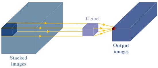
Figure 5.
The diagram of 3D convolution.
3.3.2. Target Enhancement by 3D Convolution
The key to 3D convolution is the determination of the kernel parameters, and different kernels will lead to different results. The corresponding kernel parameters are calculated according to the motion vector of the target and the number of frames stacked. Then, the target energy can be accumulated along its trajectory by 3D convolution. In addition, there are different kernels for different targets because of their different motion states. Finally, the enhancement results can be obtained by local processing.
The kernel size is determined adaptively by the motion vector of the target and the number of frames stacked, where is the number of frames stacked and is calculated by the detected optical flow:
where and are calculated in the previous section.
The enhancement by 3D convolution for a target can be expressed as
where denotes the function of 3D convolution, denotes the kernel determined by , is the number of stacked images and is the input images. And is the enhanced window, forming the resulting images . Finally, the output images are obtained with background subtraction and blind pixel suppression:
where is the region of size and denotes the gray value at the center of in the image of , and .
The results of the enhancement by 3D convolution are shown in Figure 6.
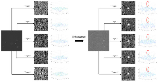
Figure 6.
The enlarged view of targets and the 3D display of them in original and enhanced images.
4. Experiments
To analyze the enhanced results of the dim moving multi-target by the proposed algorithm, qualitative and quantitative experiments were conducted. Meanwhile, this algorithm was compared with other classic enhancement methods, including the improved top-hat algorithm [42], traditional dynamic inter-frame filtering [43], the 3DCFSI-based method [24] and the ECA method [20] to test the performance.
4.1. Experimental Setup
4.1.1. Evaluation Metrics and Test Images
As per usual, the signal-to-noise ratio (SNR) was used to measure the quality of the image with the targets, which was defined as the ratio of the average power of the targets to the average power of the noise [44]:
where was the average of the peaks of all targets and was the background’s gray value. And was the standard deviation of the image, which referred to the noise. Furthermore, in this paper, we took the SNR gain as the index of the algorithm’s performance, which was defined as
where represented the SNR of the output image, and represented the SNR of the input image. And the higher the SNR gain was, the greater the effect of the enhancement algorithm.
In addition, the precision (P) and the recall (R) were used to measure the application of the algorithm to the multi-target case:
where was the number of true-targets detected as targets, was the number of false-targets detected as targets and was the number of true-targets not detected as targets.
Considering the difficulty obtaining the real space-based infrared images, we used the long-wave infrared camera (LWIR) to shoot the background and then added the simulated targets. At the same time, the effect of turntable jitter was considered. The information of the images including the background characteristic, the target characteristic and the noise characteristic was consistent with the analysis in Section 2. The velocities of the simulated targets were all in the range of 0.5~1.5 pixel/frame, and the sizes of the targets were all in the range of ~.
4.1.2. The Analysis of Parameters
There were several parameters in the proposed algorithm, and some of them could be set according to the easy experiments and the experience: the energy collected area , the maximum filtering area , the number of frames of the temporal mean filter , the parameter in the thresholding segmentation and the number of frames in the interval when using the optical flow. In addition, we set the number of frames used for the 3D convolution as . In addition, there was a crux parameter that had the threshold in the connected component detection, which was closely related to the performance of the algorithm. To analyze the influence of this value on the algorithm, 8 types of test images were adopted, which are described in Table 1. The target states in each sequence, including the velocity, direction, SNR and size of the targets, are different. And the SNR shown in the table is the combined SNR of all the targets in the whole image.

Table 1.
A detailed description of eight infrared sequences.
The threshold in the connected component detection was the key to judge whether the connected component was the thick stripe of the target trajectory. If this value was too small, it would not only detect the true-targets but also detect other interference, which would be mistaken for the targets in subsequent processing. If this value was too large, some low-weight thick stripes of the target trajectories would be removed as clutter, which could not be enhanced. Figure 7 shows the curves of the precision (P), the recall (R) and the SNR gain (SNRG) after the processing with different values of .
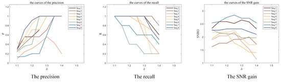
Figure 7.
The results of different evaluation metrics with different .
It is shown in Figure 7 that the value of P increased, and the value of R decreased as the value of increased. At the same time, the value of SNRG went up first and then went down or all the way down. That was because the small value of led to the false judgement, and then the P and SNRG got smaller. And the large value of led to the missed judgement, and then the R and SNRG got smaller. In addition, the SNRG peaked when was moderate, making both the P and R large. It was explained that the performance of the algorithm would decrease when the value of was too small or too large.
4.2. Validation of the Algorithm
4.2.1. The Influence of Missed and False Judgement on the Algorithm
Based on the definition in Section 4.1.1, P and R were important indexes of the algorithm, which were caused by the missed and false judgement of the targets. As per usual, R < 100% meant missed judgement and P < 100% meant false judgement. To analyze the impact of these two types of events on the performance of the algorithm, we took Seq.4 in Table 1 as an example and assumed the various cases by adjusting the parameters.
As is shown in Table 2, it can be seen from Nos. 4~5 that the smaller the value of R, the smaller the SNRG. And it can be seen from Nos. 1~2 that the value of P had little influence on the SNRG. It proved that both the missed judgement and the false judgement would degrade the performance of the algorithm. In addition, the data in Table 2 also show that R had a greater impact on the performance of the algorithm, which meant the consequences of missed judgement were even worse. That was because once the judgement was missed, the missed targets could not be processed in the following steps, and then the targets could not be enhanced, leading to the degradation of the performance of the algorithm. In addition, the false judgement was to regard the clutter or noise as the targets, but because the clutter and noise were random in the sequence images, their energy could not be accumulated by the 3D convolution. Then, the false judgement could not cause the false enhancement and had less effect on the algorithm. However, too much false judgement could also affect the accuracy of the optical flow, leading to the degradation of the performance of the algorithm.
Table 2.
The results of the algorithm in the case of missed or false judgement of the targets.
Therefore, both the theory and experiments prove that this algorithm is less affected by false judgement, that is, it has strong robustness to false enhancement.
4.2.2. The Results of the Algorithm
To show the results of the algorithm under different conditions, we processed the 8 types of images in Table 1 and the enhanced images are shown in Figure 8, where the targets are marked with a rectangle. In addition, the evaluation metrics are shown in Table 3.
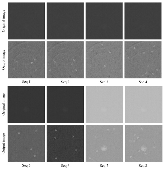
Figure 8.
The enhancement results of different types of images.
Table 3.
The results of different images processed by the algorithm.
Through the visual comparison in Figure 8, the blind pixels were extremely bright and the targets were completely invisible in the original image, while most of the blind pixels were suppressed and the targets were revealed in the output image. It proved that the targets could be enhanced by the proposed algorithm under different conditions. It also can be seen in Table 3 that the SNR of the image was significantly improved after the processing. In addition, Table 3 also shows the degradation of the enhanced performance when the SNR of the input image decreased. This was because the low SNR could lead to the increase in missed judgements and false judgements. Meanwhile, it was shown that the algorithm was affected when there were more targets in the input image.
To further explain the adaptive enhancement of the proposed algorithm to the multi-targets, Seq.4 in Table 1 was adopted to show the processing results of each target.
As is shown in Figure 9, the targets were difficult to identify in the original image, and all the targets were revealed in the output image, showing that they were extremely enhanced by the algorithm. Meanwhile, the 3D display of the targets also showed that the energy of the targets was effectively increased. In addition, it is shown in Table 4 that the SNRG of each target was much bigger than 1, which meant all the targets with a different size, velocity and SNR were enhanced reliably by the proposed algorithm. In addition, the SNR could reach times after frames were processed by 3D convolution according to the energy accumulation theory of targets [37]. As we set to 5 in the experiments that were described in Section 4.1.2, then the theoretical value of the SNRG should be 2.24. Therefore, the proposed algorithm worked well so that the result was close to the ideal value.
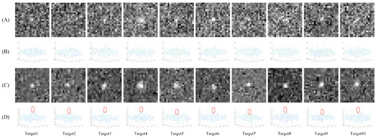
Figure 9.
The enhancement results of the multi-targets. (A) shows the original targets. (B) shows the 3D display of them. (C) shows the enhanced targets, and (D) shows the corresponding 3D displays of them, and the red oval represents the target.
Table 4.
The results of each target in an image processed by the algorithm.
4.3. Comparison
To better evaluate the performance of the proposed algorithm, we compared it with other methods for target enhancement. In the comparison experiments, the improved top-hat algorithm [41], traditional dynamic inter-frame filtering [42], 3DCFSI-based method [24] and ECA method [20] were applied. However, the 3DCFSI-based method and ECA method were not robust to false enhancement at all as they failed in the presence of blind pixels. Take the 3DCFSI as an example; as shown in Figure 10, there are several blind pixels in the original image, which has a large gray value, and the targets are submerged. When the algorithm is used to enhance the targets, the blind pixel will be misjudged as the target, so the real targets cannot be enhanced effectively.
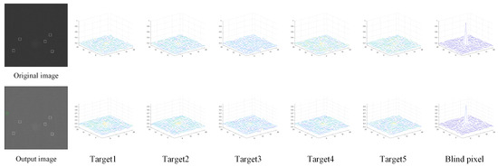
Figure 10.
Failure result of 3DCFSI affected by blind pixels.
In that case, we improved the two algorithms, adding the suppression of blind pixels. Then, the performance of the SNRG was compared with the proposed algorithm and the results are shown in Table 5. Meanwhile, the output images are shown in Figure 11, which were all displayed after blind pixels suppression in order to make the results clearer.
Table 5.
Comparison of SNR gain for five methods.
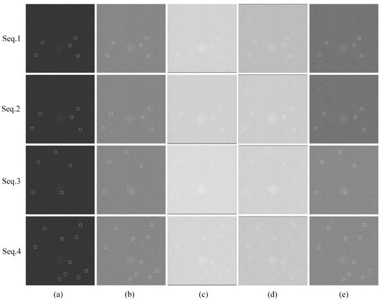
Figure 11.
Visual comparison between typical methods and proposed algorithm. Squares represent the targets. (a) The raw images of Seq.1-Seq.4, respectively. (b–e) are the enhanced results of improved top-hat algorithm, DPA-based energy accumulation, 3DCFSI-based method, ECA method and proposed algorithm, respectively.
As shown in Figure 11 and Table 5, the improved top-hat algorithm had little effect and could not enhance the targets effectively. The traditional dynamic inter-frame filtering did some work so that both the visual and quantitative results were fairly good, but it caused target trailing and energy dispersion. Then, the 3DCFSI-based method and ECA method performed well after the suppression of the blind pixels. However, they were fatally affected by false judgement. The proposed algorithm showed the best performance in both the qualitative and quantitative results. The contrast between the targets and the surrounding pixels was significantly improved, and the center of the target hardly changed and the energy was not diffused. In addition, the SNRG was greater than the others in all the sequences. And it had a strong robustness that could deal with the interference of blind pixels and noise adaptively.
4.4. Experiments on Real Data
To make our experiment more convincing, we used the real data to validate our algorithm. We used the shortwave infrared camera to observe the stars in different sky regions and obtained 3 sets of images, where several stars appeared in the field of view at the same time. Then, the enhancement algorithm was used to enhance all the stars in the images and to improve the SNR. The results are shown in Figure 12, where the stars are marked with a rectangle. In addition, the description of the images and the evaluation metrics are shown in Table 6.
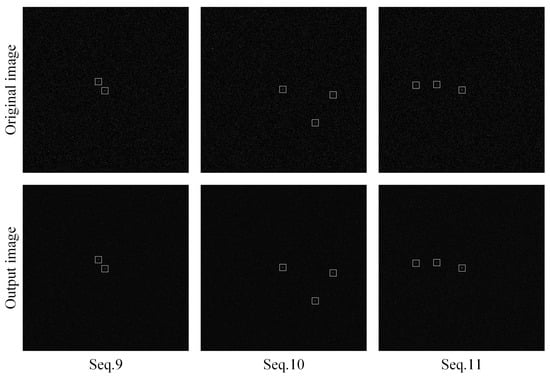
Figure 12.
The enhancement results of images with stars.
Table 6.
The description of images with stars and the results of them processed by the algorithm.
As shown in Figure 12, the blind pixels were removed and the noise was reduced, while the stars were enhanced in the output images. It also can be seen in Table 6 that the SNR of the image was significantly improved after the processing. In conclusion, both the qualitative and quantitative results proved the effectiveness of our algorithm with real data. However, there are some differences between this scene and space-based infrared detection. Generally, the stars are brighter than the space targets, so the SNR of the star image is higher than that of the target image. In addition, stars are stationary such that the motion of a star can only be simulated by the motion of the camera. Thus, the moving state of all the stars is the same, which is different from the targets. Therefore, we will also use on-orbit data to further validate our algorithm in the future.
5. Conclusions
This paper investigates the target enhancement task in a space-based background. The problems and challenges of the task are summarized as the stability at a low SNR, adaptability to multiple targets and robustness for false enhancement. A new enhancement method for a dim moving multi-target with strong robustness for false enhancement is proposed to meet these requirements. The algorithm is mainly based on multi-target localization, motion detection by optical flow and 3D convolution. On this basis, long-wave infrared images with simulated targets are used to evaluate the performance of the algorithm. It has been proved that each target in the image can be enhanced effectively and the SNR can be improved significantly under different conditions. The SNR gain can reach two by convolving five images in 3D. Meanwhile, both the theoretical analysis and experimental results show that this algorithm is less affected by the wrong judgement of the targets. In addition, the proposed algorithm has outstanding performance compared to other methods.
In the traditional image sequences, only the spatio-temporal information is included, but the multi-spectral image can provide more effective information [45,46], which can further improve the adaptability of the algorithm. Thus, we will conduct some research on it in the future.
Author Contributions
Conceptualization, P.R. and Y.Z.; data curation, Y.Z.; formal analysis, Y.Z.; funding acquisition, P.R.; investigation, Y.Z. and X.C.; methodology, P.R. and X.C.; project administration, X.C.; resources P.R. and L.J.; software, Y.Z. All authors have read and agreed to the published version of the manuscript.
Funding
This research was funded by [National Natural Science Foundation of China] grant number [62175251].
Data Availability Statement
Not applicable.
Conflicts of Interest
The authors declare no conflict of interest.
References
- Gonzalez, R.C.; Woods, R.E. Digital Image Processing; Prentice Hall International: Hoboken, NJ, USA, 2002; Volume 28, pp. 484–486. [Google Scholar]
- Kweon, Z. Edge directional 2D LMS filter for infrared small target detection. Infrared Phys. Technol. 2012, 55, 137–145. [Google Scholar]
- Seyed, M.F.; Reza, M.M.; Mahdi, N. Flying small target detection in IR images based on adaptive toggle operator. IET Comp. Vis. 2018, 12, 527–534. [Google Scholar]
- Jiang, D.; Huo, L.; Lv, Z.; Song, H.; Qin, W. A Joint Multi-Criteria Utility-Based Network Selection Approach for Vehicle-to-Infrastructure Networking. IEEE Trans. Intell. Transp. Syst. 2018, 19, 3305–3319. [Google Scholar] [CrossRef]
- Bai, X.; Zhou, F. Hit-or-miss transform based infrared dim small target enhancement. Opt. Laser Technol. 2011, 43, 1084–1090. [Google Scholar] [CrossRef]
- Bai, X. Morphological operator for infrared dim small target enhancement using dilation and erosion through structuring element construction. Opt. Int. J. Light Electron Opt. 2013, 124, 6163–6166. [Google Scholar] [CrossRef]
- Bai, X.; Zhou, F.; Xue, B. Infrared dim small target enhancement using toggle contrast operator. Infrared Phys. Technol. 2012, 55, 177–182. [Google Scholar] [CrossRef]
- Zhou, J.; Lv, H.; Zhou, F. Infrared small target enhancement by using sequential top-hat filters. Int. Soc. Opt. Photonics 2014, 9301, 417–421. [Google Scholar]
- Guofeng, Z.; Hamdulla, A. Adaptive Morphological Contrast Enhancement Based on Quantum Genetic Algorithm for Point Target Detection. Mob. Netw. Appl. 2020, 2, 638–648. [Google Scholar] [CrossRef]
- Qi, S.; Ma, J.; Li, H.; Zhang, S.; Tian, J. Infrared small target enhancement via phase spectrum of Quaternion Fourier Transform. Infrared Phys. Technol. 2014, 62, 50–58. [Google Scholar] [CrossRef]
- Tan, J.H.; Pan, A.C.; Liang, J.; Huang, Y.H.; Fan, X.Y.; Pan, J.J. A new algorithm of infrared image enhancement based on rough sets and curvelet transform. In Proceedings of the 2009 International Conference on Wavelet Analysis and Pattern Recognition, Baoding, China, 12–15 July 2009; IEEE: Piscataway, NJ, USA, 2009. [Google Scholar]
- Zhao, J.; Qu, S. The Fuzzy Nonlinear Enhancement Algorithm of Infrared Image Based on Curvelet Transform. Procedia Eng. 2011, 15, 3754–3758. [Google Scholar] [CrossRef][Green Version]
- Qiang, Z.; Pan, W.J.; Zhu, X.P.; Xuan, W. Enhancement Method for Infrared Dim-Small Target Images Based on Rough Set. In Proceeding of 2017 4th International Conference on Information Science and Control Engineering (ICISCE), Changsha, China, 21–23 July 2017; IEEE Computer Society: Washington, DC, USA, 2017. [Google Scholar]
- Yong, Y.; Wang, B.; Zhang, W.; Peng, Z. Low-contrast small target image enhancement based on rough set theory. Proc. SPIE 2007, 6833, 639–644. [Google Scholar]
- Qi, S.; Ming, D.; Ma, J.; Sun, X.; Tian, J. Robust method for infrared small-target detection based on Boolean map visual theory. App. Opt. 2014, 53, 3929–3940. [Google Scholar] [CrossRef] [PubMed]
- Zhu, B.; Xin, Y. Effective and robust infrared small target detection with the fusion of poly directional first order derivative images under facet model. Infrared Phys. Technol. 2015, 69, 136–144. [Google Scholar]
- Wei, Y.; You, X.; Li, H. Multiscale patch-based contrast measure for small infrared target detection. Patt. Recog. 2016, 58, 216–226. [Google Scholar] [CrossRef]
- Deng, H.; Sun, X.; Liu, M.; Ye, C.; Zhou, X. Infrared small-target detection using multiscale gray difference weighted image entropy. IEEE Trans. Aerosp. Electron. Syst. 2016, 52, 60–72. [Google Scholar] [CrossRef]
- Ma, T.; Shi, Z.; Jian, Y.; Liu, Y.; Xu, B.; Zhang, C. Rectilinear-motion space inversion-based detection approach for infrared dim air targets with variable velocities. Opt. Eng. 2016, 55, 33102. [Google Scholar] [CrossRef]
- Ma, T.; Wang, J.; Yang, Z.; Ku, Y.; Ren, X.; Zhang, C. Infrared small target energy distribution modeling for 2D subpixel motion and target energy compensation detection. Opt. Eng. 2022, 61, 013104. [Google Scholar] [CrossRef]
- Reed, I.S.; Gagliardi, R.M. A recursive moving-target-indication algorithm for optical image sequences. IEEE Trans. Aerosp. Electron. Syst. 1990, 26, 434–440. [Google Scholar] [CrossRef]
- Li, M.; Zhang, T.; Yang, W.; Sun, X. Moving weak point target detection and estimation with three-dimensional double directional filter in IR cluttered background. Opt. Eng. 2005, 44, 107007. [Google Scholar] [CrossRef]
- Zhang, T.; Li, M.; Zuo, Z.; Yang, W.; Sun, X. Moving dim point target detection with three-dimensional wide-to-exact search directional filtering. Pattern Recognit. Lett. 2007, 28, 246–253. [Google Scholar] [CrossRef]
- Ren, X.; Wang, J.; Ma, T.; Bai, K.; Ge, M.; Wang, Y. Infrared dim and small target detection based on three-dimensional collaborative filtering and spatial inversion modeling. Infrared Phys. Technol. 2019, 101, 13–24. [Google Scholar] [CrossRef]
- Tonissen, S.M.; Evans, R.J. Performance of dynamic programming techniques for Track-Before-Detect. IEEE Trans. Aerosp. Electron. Syst 1996, 32, 1440–1451. [Google Scholar] [CrossRef]
- Arnold, J.; Shaw, S.W.; Pasternack, H. Efficient target tracking using dynamic programming. IEEE Trans. Aerosp. Electron. Syst. 2002, 29, 44–56. [Google Scholar] [CrossRef]
- Orlando, D.; Ricci, G.; Bar-Shalom, Y. Track-Before-Detect Algorithms for Targets with Kinematic Constraints. IEEE Trans. Aerosp. Electron. Syst. 2011, 47, 1837–1849. [Google Scholar] [CrossRef]
- Sun, X.; Liu, X.; Tang, Z.; Long, G.; Yu, Q. Real-time visual enhancement for infrared small dim targets in video. Infrared Phys. Technol. 2017, 83, 217–226. [Google Scholar] [CrossRef]
- Guo, Q.; Li, Z.; Song, W.; Fu, W. Parallel Computing Based Dynamic Programming Algorithm of Track-before-Detect. Symmetry 2018, 11, 29. [Google Scholar] [CrossRef]
- Li, Y.; Wei, P.; Gao, L.; Sun, W.; Zhang, H.; Li, G. Micro-Doppler Aided Track-Before-Detect for UAV Detection. In Proceedings of the IGARSS 2019, 2019 IEEE International Geoscience and Remote Sensing Symposium, Yokohama, Japan, 28 July–2 August 2019; pp. 9086–9089. [Google Scholar]
- Wei, H.; Tan, Y.; Jin, L. Robust Infrared Small Target Detection via Temporal Low-Rank and Sparse Representation. In Proceedings of 2016 3rd International Conference on Information Science and Control Engineering (ICISCE), Beijing, China, 8–10 July 2016; IEEE: Piscataway, NJ, USA, 2016. [Google Scholar]
- Li, J.; Li, S.J.; Zhao, Y.J.; Ma, J.N.; Huang, H. Background Suppression for Infrared Dim and Small Target Detection Using Local Gradient Weighted Filtering. In Proceedings of the International Conference on Electrical Engineering and Automation, Hong Kong, China, 24–26 June 2016. [Google Scholar]
- Hong, Z.; Lei, Z.; Ding, Y.; Chen, H. Infrared small target detection based on local intensity and gradient properties. Infrared Phys. Technol. 2017, 89, 88–96. [Google Scholar]
- Ma, T.; Shi, Z.; Yin, J.; Baoshu, X.; Yunpeng, L. Dim air target detection based on radiation accumulation and space inversion. Infrared Phys. Technol. 2015, 44, 3500–3506. [Google Scholar]
- Yang, T.; Zhou, F.; Xing, M. A Method for Calculating the Energy Concentration Degree of Point Target Detection System. Spacecr. Recovery Remote Sens. 2017, 38, 41–47. [Google Scholar] [CrossRef]
- Jia, L.J. Research on Key Technologies of On-satellite Processing for Infrared Dim Small Target; University of Chinese Academy of Sciences: Beijing, China, 2022. [Google Scholar]
- Pan, H.B.; Song, G.H.; Xie, L.J.; Zhao, Y. Detection method for small and dim targets from a time series of images observed by a space-based optical detection system. Opt. Rev. 2014, 21, 292–297. [Google Scholar] [CrossRef]
- Li, H.; Chen, Q. The Technique of the Multi-frame Image Accumulation and Equilibration with Infrared Thermal Imaging System. Las. Infrared 2005, 35, 978–990. [Google Scholar]
- Lucas, B.D.; Kanade, T. An Iterative Image Registration Technique with an Application to Stereo Vision. In Proceedings of the 7th International Joint Conference on Artificial Intelligence; Morgan Kaufmann Publishers Inc.: Burlington, MA, USA, 1997. [Google Scholar]
- Ji, S.; Xu, W.; Yang, M.; Yu, K. 3D Convolutional Neural Networks for Human Action Recognition. IEEE Trans. Pattern Anal. Mach. Intell. 2013, 35, 221–231. [Google Scholar] [CrossRef] [PubMed]
- Tran, D.; Bourdev, L.; Fergus, R.; Torresani, L.; Paluri, M. Learning Spatiotemporal Features with 3D Convolutional Networks; IEEE: Piscataway, NJ, USA, 2015. [Google Scholar]
- Bai, X.; Zhou, F.; Jin, T.; Xie, Y. Infrared small target detection and tracking under the conditions of dim target intensity and clutter background. In Proceedings of the MIPPR 2007: Automatic Target Recognition and Image Analysis and Multispectral Image Acquisition; International Society for Optics and Photonics: Washington, DC, USA, 2007. [Google Scholar]
- Chen, Q. Dynamic Inter-frame Filtering in IR Image Sequences. J. Nanjing Univ. Sci. Technol. 2003, 27, 653–656. [Google Scholar]
- Wang, X.; Wang, C.; Zhang, Y. Research on SNR of Point Target Image. Electron. Opt. Control. 2010, 17, 18–21. [Google Scholar]
- Xiong, F.; Zhou, J.; Qian, Y. Material Based Object Tracking in Hyperspectral Videos. IEEE Trans. Image Process. 2020, 29, 3719–3733. [Google Scholar] [CrossRef]
- Yang, X.; Zhao, M.; Shi, S.; Chen, J. Deep Constrained Energy Minimization for Hyperspectral Target Detection. IEEE J. Sel. Top. Appl. Earth Observ. Remote Sens. 2022, 15, 8049–8063. [Google Scholar] [CrossRef]


Disclaimer/Publisher’s Note: The statements, opinions and data contained in all publications are solely those of the individual author(s) and contributor(s) and not of MDPI and/or the editor(s). MDPI and/or the editor(s) disclaim responsibility for any injury to people or property resulting from any ideas, methods, instructions or products referred to in the content. |
© 2023 by the authors. Licensee MDPI, Basel, Switzerland. This article is an open access article distributed under the terms and conditions of the Creative Commons Attribution (CC BY) license (https://creativecommons.org/licenses/by/4.0/).